Randomised benchmarking for characterizing and forecasting correlated processes

A major challenge in building near-term quantum computers is noise [1, 2, 3]. As the number of qubits and the depths of quantum circuits scale up, the fidelity of the output quantum state decreases rapidly, restricting current experiments to low depths [4, 5, 6], or few qubits [7]. A quantum device can be affected by both spatially and temporally correlated noise. Correlated noise can be more harmful then uncorrelated one for scalable quantum error mitigation [8, 9], and can lower the threshold of error correcting codes [10, 11]. Efficient tools to characterize correlated noise are essential for the development of scalable quantum computing technologies.

A variety of techniques have been developed for characterizing Markovian noises, including spatially correlated ones, such as quantum process tomography (QPT) [12, 13], gate set tomography [14, 15] and randomized benchmarking (RB) [16, 17, 18, 19, 20]. RB is a highly economical method that consists of averaging over random sequences of gates to estimate the error rates within a given device.

The process tensor framework was recently introduced to expand the applicability of the above tools to time-correlated or non-Markovian noise [21, 22]. A process tensor is a complete positive mapping from any sequence of $k$ quantum operations to a final state of the system. Similar to QPT, the process tensor can be systematically reconstructed with process tensor tomography (PTT), where one applies all the possible sequences of linearly independent quantum operations and performs quantum state tomography [23]. Unlike RB, PTT yields detailed information about the noise, which can be used to improve the performance of the quantum device [24]. However, the detailed characterization of complex noise is far more expensive than RB. PTT requires a number of measurements that grows exponentially with $k$. Meanwhile, it is possible to get around this exponential scaling by exploiting the process tensor’s natural form as a matrix product density operator with a finite bond dimension [22, 25, 26], which motivates efficient heuristic PTT schemes based on one-dimensional tensor network states [27, 28, 29]. Alternatively, one may apply recently-developed shadow-based schemes [30].

In this work, we develop a method to reconstruct the process tensors by applying supervised machine learning methods to RB data. Our scheme thus inherits the simplicity of RB while capturing the complexity of multi-time non-Markovian system dynamics. It enables one to characterize the process, including concrete measures of non-Markovianity, while its computational cost is related to the memory size of the process, which is often small for real quantum hardware [24].

As a proof of principle, we demonstrate our scheme on a superconducting quantum processor, where we couple a “system” qubit to an “environment” qubit with tunable coupling strength, going from weak to strong, resulting in system dynamics from nearly Markovian to highly non-Markovian. We observe a sharp change in learning accuracy between these two regimes; very high learning accuracy in the Markovian regime, and generally lower accuracy in the highly non-Markovian regime, although this can be systematically improved by using larger memory models. In both cases, we can predict future dynamics beyond the times used for training.

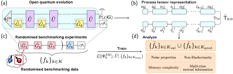
Open quantum evolution model and the process tensor framework. Stationary classical non-Markovian processes can always be written as hidden Markov models [31, 32]. Similarly, for quantum processes with time-independent noise, one could reconstruct a quantum version of the hidden Markov model, referred to as the open quantum evolution (OQE) model, which describes the overall unitary dynamics of the system coupled to a minimal environment [33], which we call memory $M$. Once obtained, the OQE model contains all the information of the system dynamics, which can be used to compute process tensors of any steps and predict all the future dynamics.

Without loss of generality, we assume a pure system-memory ($SM$) initial state $|\Psi_{0}^{SM}\rangle$. We consider the discretized $SM$ dynamics from time steps $t_{1}$ to $t_{k}$ ($t_{0}=0$), and denote the unitary $SM$ evolutionary operator from $t_{j-1}$ to $t_{j}$ as $\hat{U}_{j,j-1}$. At each step $j$ we apply a quantum operation $\hat{G}_{j}$ (unitary operation or measurement) on $S$. The overall $SM$ dynamics can be written as

which is shown in Fig. 1(a). Eq. (1) also defines the process tensor $\hat{\Upsilon}_{k:0}$ as a mapping from initial state of the system $\hat{\rho}^{S}_{0}$, together with $\{\hat{G}_{i}\}_{i=1}^{k}\stackrel{{\scriptstyle\mathrm{def}}}{{=}}\{\hat{G}_{1},\dots,\hat{G}_{k}\}$, into the final state $\hat{\rho}^{S}_{k}={\rm tr}_{M}(|\Psi_{k}^{SM}\rangle\langle\Psi_{k}^{SM}|)$, as shown in Fig. 1(b) (See Supplementary for detailed construction of $\hat{\Upsilon}_{k:0}$ from OQE [34]). $\hat{\Upsilon}_{k:0}$ contains all the observable information of the $k$-step system dynamics and is uniquely defined (in contrast OQE is not unique [33]). In the next, we focus on time-independent noise with $\hat{U}_{j:j-1}=\hat{U}$ for any $j$. In this case, the open quantum dynamics is completely determined by $|\Psi_{0}^{SM}\rangle$ and $\hat{U}$, and our goal is to determine them by performing RB on the system only.

Reconstructing the OQE model with RB. For RB one first randomly generates $n$ sequences, denoted as $\{\{\hat{G}^{1}_{i}\}_{i=1}^{k},\dots,\{\hat{G}^{n}_{i}\}_{i=1}^{k}\}$, where in each sequence the last operation $\hat{G}_{k}^{l}$ is understood as the undo gate $\hat{G}_{k}^{l}=(\hat{G}_{k-1}^{l}\cdots\hat{G}_{2}^{l}\hat{G}_{1}^{l})^{\dagger}$ used to isolate the noise effects. Then the RB protocol proceeds as follows: (1) Preparing an initial state $\hat{\rho}^{S}_{0}$ of the system; (2) Applying each $\{\hat{G}^{l}_{i}\}_{i=1}^{k}$ onto $\hat{\rho}^{S}_{0}$ to obtain the final state $\hat{\rho}^{S,l}_{k}$ and measuring $f^{l}_{k}={\rm Tr}(\hat{M}\hat{\rho}^{S,l}_{k})$ for a positive operator-valued measure element $\hat{M}$; (3) Computing the average $F_{k}=\sum_{l=1}^{n}f_{k}^{l}/n$ and repeating (1) and (2) for different $k$. For Markovian noise that is also gate-independent, $F_{k}$ can be well approximated by an exponential decay $F_{k}=ap^{k}+b$ where $a$, $b$ and $p$ are constants [19, 20]. For non-Markovian noise, instead, non-exponential behavior of $F_{k}$ is expected in general [35]. The RB protocol can be naturally understood in the process tensor framework, which is demonstrated in Fig. 1(c) in correspondence with Fig. 1(a).

Based on the RB data, we propose a variational scheme to reconstruct the hidden OQE model by minimizing the mean square loss between the predicted outcomes $\tilde{f}^{l}_{k}=\langle\Psi^{SM,l}_{k}|\hat{M}|\Psi^{SM,l}_{k}\rangle$ and the experiment outcomes $f^{l}_{k}$:

where $K_{{\rm train}}$ is the set of $k$ used for training. We use the BFGS optimizer [36], with $\hat{U}$ parameterized as in Ref. [37] and randomly initialized with a predefined memory size $\chi$. The gradient is computed by automatic differentiation [38]. Once an optimal OQE model has been obtained, one can use it to predict the output quantum state $\hat{\rho}^{S}_{k^{\prime}}$ of the system for any sequence $\{\hat{G}_{i}\}_{i=1}^{k^{\prime}}$ ($k^{\prime}$ may not be in $K_{{\rm train}}$) as shown in Fig. 1(d).

Experimental setup. To demonstrate our method, we apply it to reconstruct temporally correlated noise on a superconducting quantum processor. We use two capacitive-coupled transmon qubits, one as system ($S$) and the other as environment ($E$). Note that we have differentiated between the physical environment $E$ of the quantum processor and memory $M$ that goes into the OQE, where $M$ includes the qubit $E$ and can include other effects that we cannot directly control. The $SE$ Hamiltonian is $\hat{H}=J(\hat{\sigma}^{+}_{S}\hat{\sigma}^{-}_{E}+\hat{\sigma}^{+}_{E}\hat{\sigma}^{-}_{S})+h_{S}\hat{\sigma}^{z}_{S}+h_{E}\hat{\sigma}^{z}_{E}$, where $J$ is the coupling strength, $h_{S/E}$ is the local energy for the system or environment qubit. Once again, we highlight the fact that a one qubit memory is sufficient for modelling realistic quantum computers [23, 25, 24].

We apply the standard RB protocol on $S$ as depicted in Fig. 1(c). The initial state is chosen as $\hat{\rho}^{S}_{0}=|0^{S}\rangle\langle 0^{S}|$. While it is not necessary for our algorithm, for a more straightforward implementation we consider that the $SM$ initial state is separable: $|\Psi_{0}^{SM}\rangle=|0^{S}\rangle\otimes|\Psi_{0}^{M}\rangle$, and we can simplify Eq. (2) by fixing $|\Psi_{0}^{M}\rangle=|0^{M}\rangle$ without loss of generality (one can change the environment basis without any observable effects). As a result, only $\hat{U}$ remains to be determined. To tune the system dynamics from Markovian to non-Markovian, one needs to tune the coupling between $S$ and $M$. In our experiment, $J$ is kept as a constant, but we tune the effective coupling strength $\gamma_{{\rm eff}}=2J^{2}/\Delta h$ by changing the imbalance $\Delta h=h_{S}-h_{E}$ via the voltage bias $V_{bias}$, as shown in Fig. 2(a).

The reconstruction accuracy. In our experiment, each gate operation takes about $20\times i$ ns, with $i=1,2,3$ depending on the number of native gates obtained through Epstein decomposition [39]. The idle time between gates is set to be $100$ ns. In this way, the duration between successive time steps in OQE could be slightly different, which would break our assumption of time-independent $\hat{U}$. Nevertheless, our results later show that our reconstructed models are still accurate. For each $V_{bias}$ in Fig. 2(a), we independently prepare two datasets with $k\in[2,40]$ and $k\in[2,60]$ respectively, and for each $k$ we prepare $n=200$ data pairs. We take $60\%$ (for each $k$) of the first dataset for training ($K_{{\rm train}}$), and the rest of the first dataset (denoted as $K_{{\rm val}}$ instead) as well as the whole second dataset ($K_{{\rm pred}}$) for testing. For training, we ramp up $\chi$ (dimension of $M$) from $1$ to $6$ such that our model becomes increasingly more expressive. For each $\chi$, we use the BFGS optimizer with at most $200$ iterations to find an optimal $\hat{U}$ as a $2\chi\times 2\chi$ unitary matrix. We run the optimization for each instance for $5$ times and choose the one with the lowest loss value as our final result.

In Fig. 2(c,d), we show the loss values for the two testing datasets $K_{{\rm val}}$ and $K_{{\rm pred}}$ respectively. In both cases, we can see that for $V_{bias}\leq 0.2$ we can obtain very low loss with a small $\chi$, while for $V_{bias}>0.2$ one needs larger $\chi$ to reach lower loss. Importantly, the model trained for $K_{{\rm train}}=[2,40]$ can be well generalized to $K_{{\rm pred}}=[2,60]$, which shows that our method is capable of predicting future dynamics. In addition, the OQE trained with $\chi=4$ works better for $K_{{\rm pred}}$ than $\chi=5,6$, especially for $V_{bias}<0.22$, which is a sign of overfitting in the near Markovian regime for large $\chi$.

To better visualize the power of our trained OQE model, in Fig. 2(b) we directly plot the average predicted measurement outcomes $\tilde{F}_{k}=\sum_{l=1}^{n}\tilde{f}_{k}^{l}/n$ from the OQE reconstructed with $\chi=5$, compared to $F_{k}$ obtained from experiment for $K_{{\rm pred}}$. We can see that in the near-Markovian regime with $V_{bias}=0.04,0.16$, there is a very good matching between them, while in the non-Markovian regime, the discrepancy becomes larger, especially for larger $k$. There is a constant bias between the predicted values and the experimental results for large $k$, which indicates a measurement bias from the experiment that has not been taken into account in our method.

Quantifying the properties of multi-time processes. The process tensor, obtained from the OQE model, is a Hermitian, positive, unit-trace multipartite matrix. In other words, it is a multi-time density matrix whose correlations quantify non-Markovianity. Here, we consider three different properties of the process tensor: 1) its entropy; 2) its multipartite non-Markovianity; and 3) non-Markovianity across two times. As such, we need to define von Neumann entropy $\mathcal{S}(x):=-\mbox{tr}[\rho_{x}\log(\rho_{x})]$ and mutual information $\mathcal{I}(x,y):=\mathcal{S}(x)+\mathcal{S}(y)-\mathcal{S}(xy)$.

For the first measure, we compute the entropy of the whole process tensor $\mathcal{M}_{j}=\mathcal{S}(\hat{\Upsilon}_{j:0})$, which quantifies the level of noise in the process. For OQE, $\mathcal{M}_{j}$ is the same as the final entropy of the $M$ space, thus it is sometimes referred to as memory complexity [33] and it resembles statistical complexity of classical stochastic process [40]. The second measure quantifies the multi-time correlation between the past and the future of the process. To do so, we first vectorise the process tensor, i.e., $\hat{\Upsilon}_{k:0}\to\mbox{vec}(\hat{\Upsilon}_{k:0})/\|\hat{\Upsilon}_{k:0}\|_{2}$, with $\|\hat{\Upsilon}_{k:0}\|_{2}$ the normalisation. The entropy of a subpart $x$ of this pure state vanishes iff the process is Markovian [41]. We take $x$ to be times $0$ to $j$ and denote the entropy as $\mathcal{N}_{j}$, which captures the correlations between the past and the future. Finally, we compute the mutual information between marginals of the process tensor; from $\hat{\Upsilon}_{k:0}$, we obtain a bipartite process tensor $\hat{\Upsilon}_{x,y}$ by contracting all $o_{j}$ with $i_{j}$, i.e., inserting the identity gates at all time slots $j$. Indices $o_{x-1},o_{y-1}$ are traced out and a $\left|0\right>$ is inserted at $i_{x}$. The mutual information of $\hat{\Upsilon}_{x,y}$ quantifies four time correlation which vanishes for all Markovian processes.

The three quantities above capture different aspects of the non-Markovian process and are plotted in Fig. 3. Panels (a,b) display $\mathcal{M}_{j}$ and $\mathcal{N}_{j}$, respectively to show a sharp transition from the Markovian regime for $V_{bias}\leq 0.2$ to the non-Markovian regime for $V_{bias}>0.2$. Neither measure converges with $\chi$ for $V_{bias}>0.23$, which means that a larger $\chi$ (and more training data) may be required for the hidden OQE. Interestingly, for $V_{bias}\leq 0.2$, $\mathcal{M}_{j}$ is much larger than $\mathcal{N}_{j}$. This could mean that the underlying quantum dynamics can be well approximated by a Markovian but non-unitary process. To further examine this, we compute the mutual information for $V_{bias}=0.04$ and $V_{bias}=0.232$ respectively in panels (c,d). In the first case, the mutual information is small and gradually increases with $k$, indicating an evolution of short-range memory with the dynamics. Owing to the lower coupling, more time is needed to generate the required interaction to accumulate temporal correlations. Moreover, as one would expect, these correlations reduce with temporal separation $\Delta k$. Nevertheless, one can see that even in a low-coupling regime a coherent system can eventually develop non-Markovian features. Meanwhile, in the second case, the mutual information starts very high and quickly saturates (note the y-axis scale difference between c/d). Because we have fixed interaction with a small environment, the quantity $\mathcal{I}(1,k)$ decays exponentially. But the closer-in-time correlations maintain a large steady state with $k$ until they are slowly reduced by dissipation. Using our tools, we see that the dynamics of memory can be studied in company with the usual information provided by RB curves.

Summary. We have proposed an experimentally friendly scheme to characterize temporally correlated noise in open quantum dynamics based on data from randomized benchmarking experiments. We demonstrated our method on a superconducting quantum processor, where we tune the quantum dynamic of the system qubit from Markovian to highly non-Markovian by tuning the effective coupling strength to an environment qubit. Our results show that, close to the Markovian regime, we can reconstruct an OQE model with a very small memory size and with high prediction accuracy on the testing datasets. In the highly non-Markovian regime, the reconstruction accuracy is generally lower but can be systematically improved by using a larger memory size. In both cases the reconstructed OQE model can well predict the observed and even unobserved system dynamics. We computed three different measures of non-Markovianity using the process tensor obtained from reconstructed OQE and we find that they indeed have a close correspondence with the Markovian or non-Markovian behaviors of the system dynamics. Our method thus opens up the possibility of quantifying temporally correlated noise in quantum devices based on existing RB data.