Radio Frequency Interference Detection Using Efficient Multi-Scale Convolutional Attention UNet
Abstract
Studying the universe through radio telescope observation is crucial. However, radio telescopes capture not only signals from the universe but also various interfering signals, known as Radio Frequency Interference (RFI). The presence of RFI can significantly impact data analysis. Ensuring the accuracy, reliability, and scientific integrity of research findings by detecting and mitigating or eliminating RFI in observational data, presents a persistent challenge in radio astronomy. In this study, we proposed a novel deep learning model called EMSCA-UNet for RFI detection. The model employs multi-scale convolutional operations to extract RFI features of various scale sizes. Additionally, an attention mechanism is utilized to assign different weights to the extracted RFI feature maps, enabling the model to focus on vital features for RFI detection. We evaluated the performance of the model using real data observed from the 40-meter radio telescope at Yunnan Observatory. Furthermore, we compared our results to other models, including U-Net, RFI-Net, and R-Net, using four commonly employed evaluation metrics: precision, recall, F1 score, and IoU. The results demonstrate that our model outperforms the other models on all evaluation metrics, achieving an average improvement of approximately 5% compared to U-Net. Our model not only enhances the accuracy and comprehensiveness of RFI detection but also provides more detailed edge detection while minimizing the loss of useful signals.
keywords:
methods: data analysis - techniques: image processing.1 Introduction
Being essential for studying the universe, radio telescopes capture radio signals from the cosmos, invariably confronting Radio Frequency Interference (RFI) in the process.In light of the rapid advancement of human communication technology,signals generated by human activities are increasingly occupying a larger portion of the frequency bands. Consequently, the interference to radio observation equipment within these frequency bands has intensified and substantially compromised the quality of radio astronomy observation data (Yan et al., 2021). Therefore, in order to ensure the accuracy and validity of radio astronomy research, it is crucial to accurately detect RFI from complex radio observations.
Traditional RFI detection methods are mainly Singular Vector Decomposition (Offringa et al., 2010b), Principle Component Analysis (Zhao et al., 2013), CUMSUM (Baan et al., 2004) and SUMTHRESHOLD (Offringa et al., 2010b), which have been widely used in various radio data processing pipelines (Akeret et al., 2017a; Offringa et al., 2010a, b; Peck & Fenech, 2013). However, these traditional methods are largely influenced by human empirical factors, increasing the need for manual intervention and greatly reducing the efficiency of data processing. In addition, some new Bayesian-based statistical methods have been used for RFI mitigation in more recent studies(Leeney et al., 2023; Finlay et al., 2023).
In order to overcome the limitations of the above methods, the use of deep learning techniques based on computer vision to detect RFI has also been gradually explored. The U-Net (Ronneberger et al., 2015) model was initially used by Akeret et al. (2017b) for RFI detection. After testing on simulated single-dish data, the U-Net architecture demonstrated superior results to traditional methods.Kerrigan et al. (2019)achieved promising outcomes by combining amplitude and phase information and utilizing a fully convolutional neural network to identify RFI in HERA(DeBoer et al., 2017) data. Inspired by residual networks(He et al., 2016), Yang et al. (2020)proposed the RFI-Net model by extending the U-Net model. This model outperformed U-Net on several datasets, including FAST. In more recent studies, transfer learning(Tan et al., 2018) has also been used for RFI detection. The R-Net model, proposed by Vafaei Sadr et al. (2020), was first trained on simulated data and then fine-tuned on real data, achieving superior performance compared to U-Net.
Most existing deep learning methods have demonstrated promising results in simulating data. However, when applied to detect RFI in the real observation data from the Yunnan Observatory’s 40-meter radio telescope, these models often misclassify non-RFI as RFI and miss certain instances of RFI that go undetected, necessitating additional manual inspection. Because compared to the simple RFI types in simulated data, RFI in real data is usually more complex. To address these challenges and enhance RFI detection in real data, we propose a novel deep learning model that combines the advantages of attention mechanism and multi-scale convolutional neural networks.
In contrast to the aforementioned deep learning models, we have replaced the single-sized small convolution kernel with multiple-sized large convolution kernels, and integrated an attention mechanism into the convolutional neural network. While convolutional neural networks are effective at extracting local information, they often overlook global information. However, the inclusion of attention mechanisms assists the model in considering global information. Therefore, the combination of these elements allows our model to simultaneously handle both local and global patterns, resulting in improved detection of RFI in real data. Our model utilizes multi-scale convolutional operations to extract informative RFI features and generate corresponding feature maps. Subsequently, through the attention mechanism, the model focuses on the relevant features crucial for RFI detection, rather than processing all the information in the feature maps, thereby improving the efficiency of detection.
The structure of this paper is as follows: In Section 2,we describe the telescope used for data acquisition and provide details of the experimental data. In Section 3, the composition and functions of each module in our model are presented. Next, the details of our experiments are described in Section 4. The evaluation of the experimental results and the analysis and discussion of their reasons are addressed in Section 5. Finally, our conclusions are provided in Section 6.
2 Data

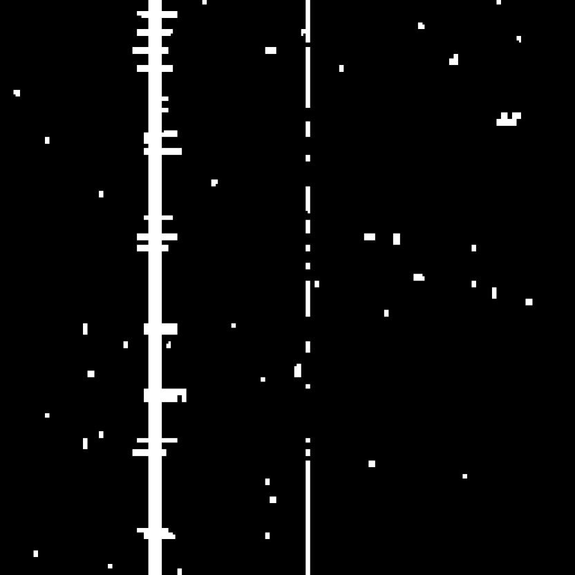
The experimental data were obtained through pulsar timing observations conducted using the Yunnan Observatory’s 40-meter radio telescope, situated in the southwestern region of China (25°01’38” N, 102°47’45” E). This telescope is equipped with a room-temperature S/X receiver and a cooled circularly polarized C-band receiver, which was installed in 2016. The system temperatures for the Yunnan Observatory’s 40-meter radio telescope in the S and C bands are 70 K and 30 K, respectively(Xu et al., 2023). Specifically designed for pulsar observation, the telescope operates within the S band (2150 MHz-2450 MHz), with a center frequency of 2256 MHz. Given the typically weak nature of pulsar signals, these are folded over a specified integration time (e.g., 30 seconds, also termed "subintegration" or "subint") aligning with the pulsar signal period for attaining clearer pulse profiles. The folded pulsar data is stored in the standard PSRFITS format(Hotan et al., 2004) for further analysis. In order to capture the characteristics of RFI comprehensively, we selected observation data from September 2016 to October 2022, which includes data from three different pulsars: PSR J0332+5434, J00358+5413, and J0437-4715. We select data with the number of subintegration greater than 90 and the number of frequency channels greater than 128 for analysis. Fig. 1 displays the time-frequency image of the actual observation data from PSR J0032+5434, where the typical RFI can be observed to be much brighter than the background noise or astronomical signals.
All the corresponding labels for the data were generated using the aoflagger algorithm(Offringa et al., 2023). Diverse strategies of aoflagger exert varied effects on identifying different types of RFI; selecting appropriate flagging strategies for respective RFI can typically yield favorable results. Consequently,when creating the ground truth, we initially employ various flagging strategies of Aoflagger to flag the data, followed by manual verification of the labels’ accuracy. Our study’s dataset encompasses 1384 data samples. Due to the relatively small size of the dataset, in order to reduce overfitting and enhance the generalizability of the model, we performed random cropping and random horizontal flipping as data augmentation operations on the training data. The size of the time-frequency images used for model training and evaluation is 256×256.
3 Method
| Layer | Operation | Input size | Output size | Kernel size | ||
| short cut | Conv | B×3×256×256 | B×64×256×256 | 1×1 | ||
| conv1 | Conv+BN+GELU | B×3×256×256 | B×32×256×256 | 3×3 | ||
| conv2 | Conv+BN | B×32×256×256 | B×64×256×256 | 3×3 | ||
| add | Add |
|
B×64×256×256 | - |
| Layer | Operation | Input size | Output size | Kernel size | ||
| stemconv | StemConv Block | B×3×256×256 | B×64×256×256 | - | ||
| eca1 | ECA Block | B×64×256×256 | B×64×256×256 | - | ||
| msca1 | MSCA Block | B×64×256×256 | B×64×256×256 | - | ||
| down sample 1 | Conv+BN+GELU | B×64×256×256 | B×128×128×128 | 2×2 | ||
| eca2 | ECA Block | B×128×128×128 | B×128×128×128 | - | ||
| msca2 | MSCA Block | B×128×128×128 | B×128×128×128 | - | ||
| down sample 2 | Conv+BN+GELU | B×128×128×128 | B×256×64×64 | 2×2 | ||
| eca3 | ECA Block | B×256×64×64 | B×256×64×64 | - | ||
| msca3 | MSCA Block | B×256×64×64 | B×256×64×64 | - | ||
| down sample 3 | Conv+BN+GELU | B×256×64×64 | B×512×32×32 | 2×2 | ||
| eca4 | ECA Block | B×512×32×32 | B×512×32×32 | - | ||
| msca4 | MSCA Block | B×512×32×32 | B×512×32×32 | - | ||
| down sample 4 | Conv+BN+GELU | B×512×32×32 | B×1024×16×16 | 2×2 | ||
| eca5 | ECA Block | B×1024×16×16 | B×1024×16×16 | - | ||
| msca5 | MSCA Block | B×1024×16×16 | B×1024×16×16 | - | ||
| up sample 1 | TransposeConv+BN+GELU | B×1024×16×16 | B×512×32×32 | 2×2 | ||
| concat 1 | Concatenate |
|
B×1024×32×32 | - | ||
| eca6 | ECA Block | B×1024×32×32 | B×1024×32×32 | - | ||
| conv1 | Conv | B×1024×32×32 | B×512×32×32 | 1×1 | ||
| msca6 | MSCA Block | B×512×32×32 | B×512×32×32 | - | ||
| up sample 2 | TransposeConv+BN+GELU | B×512×32×32 | B×256×64×64 | 2×2 | ||
| concat 2 | Concatenate |
|
B×512×64×64 | - | ||
| eca7 | ECA Block | B×512×64×64 | B×512×64×64 | - | ||
| conv2 | Conv | B×512×64×64 | B×256×64×64 | 1×1 | ||
| msca7 | MSCA Block | B×256×64×64 | B×256×64×64 | - | ||
| up sample 3 | TransposeConv+BN+GELU | B×256×64×64 | B×128×128×128 | 2×2 | ||
| concat 3 | Concatenate |
|
B×256×128×128 | - | ||
| eca8 | ECA Block | B×256×128×128 | B×256×128×128 | - | ||
| conv3 | Conv | B×256×128×128 | B×128×128×128 | 1×1 | ||
| msca8 | MSCA Block | B×128×128×128 | B×128×128×128 | - | ||
| up sample 4 | TransposeConv+BN+GELU | B×128×128×128 | B×64×256×256 | 2×2 | ||
| concat 4 | Concatenate |
|
B×128×256×256 | - | ||
| eca9 | ECA Block | B×128×256×256 | B×128×256×256 | - | ||
| conv4 | Conv | B×128×256×256 | B×64×256×256 | 1×1 | ||
| msca9 | MSCA Block | B×64×256×256 | B×64×256×256 | - | ||
| output | Conv+BN+Sigmoid | B×64×256×256 | B×1×256×256 | - |
To address the limitations of existing methods, we propose a new deep learning model for RFI detection, which we refer to as EMSCA-UNet. The network schematic diagram is shown in Fig. 2, and the detailed structure can be found in Table 2. Next, we will provide a detailed overview of the overall architecture of our proposed model and discuss the specifics of each module that constitutes this model.

3.1 Architecture of EMSCA-UNet
In constructing the backbone network of our model, we draw inspiration from the multi-scale convolutional attention mechanism (MSCA) proposed by Guo et al. (2022) and the efficient channel attention mechanism (ECA) introduced by Wang et al. (2020). The combination of these two mechanisms provides the ability for channel weight adaptation and multi-scale feature processing in RFI detection. Our model is based on a clear and effective encoder-decoder architecture. For the input data, we initially apply a StemConv block (detailed in Table 1), consisting of a dual-layer 3×3 convolution and residual connection (He et al., 2016), for preliminary processing. This design not only prevents gradient vanishing and stabilizes the training process but also extracts low-level features of RFI from the images, providing richer feature information for subsequent layers. In the subsequent encoding and decoding stages, ECA blocks are used to learn the correlations between different channels, adaptively adjusting the weight of each channel to improve the performance and efficiency of the network. Then, the channels with different weights are input into MSCA blocks to extract multi-scale features of RFI. Throughout the encoding and decoding process, we stack a series of these ECA and MSCA blocks to construct a U-shaped network structure (Ronneberger et al., 2015).
In the encoder part, we replaced the previous max pooling down-sampling method with 2×2 convolutional layers, which reduces both spatial and semantic information loss while decreasing the computational burden. In the decoder part, we restored the original image resolution gradually by using transpose convolution to preserve as much image detail as possible. High-resolution feature maps contain rich details and low-level information, but they may have negative impacts on RFI detection. On the other hand, low-resolution feature maps have higher semantic information but lack specific spatial details. Therefore, in the decoding process, we adopted skip connections similar to Unet to integrate the low-level and high-level RFI features (Ronneberger et al., 2015). Through skip connections, we can combine contextual information and multi-scale information, maintain the spatial structure and detail information of the image, compensate for the spatial information loss caused by downsampling, and improve the expressiveness and detection accuracy of the network. Since skip connections double the number of channels, we used 1×1 convolutional layers to re-model and fuse the cross-channel features in order to reduce the number of channels. In the final output layer, we used a 1×1 convolutional layer to reduce the number of channels to 1. Then, we applied the sigmoid activation function to map all results to a probability range of 0 to 1. By setting the threshold to 0.5, we obtained the output segmentation mask. To prevent overfitting, we also introduced the droppath mechanism (Huang et al., 2016) to enhance the model’s generalization ability. In this study, we set the droppath rate to 0.2. As for our model architecture, the use of a U-shaped structure is something that has been done previously; however, those approaches solely employed single-scale small convolutional kernels in their convolutional neural networks. We have replaced these small, single-scale convolutional kernels with larger, multi-scale ones and have integrated attention mechanisms into the network, which is a novelty not found in the methods we compared with. All hyperparameters in this network architecture were carefully tuned and optimized through extensive experimentation.
3.2 ECA block

| Layer | Operation | Input size | Output size | Kernel size | ||
| pool | Adaptive Average Pooling+Reshape | B×C×H×W | B×1×C | - | ||
| conv | 1D Conv | B×1×C | B×1×C | kernel_size= (1) | ||
| sigmoid | Sigmoid activation+Reshape | B×1×C | B×C×1×1 | - | ||
| multiply | Element-Wise Product |
|
B×C×H×W | - |
When observing an image, we typically pay more attention to the parts that interest us. Similarly, attention mechanisms assist neural networks in better utilizing input information. In our network, after the RFI image is processed by convolutional layers, multiple feature maps are generated at different stages. However, not all of these feature maps contribute equally to RFI detection. We should prioritize the feature maps that are more helpful for detecting RFI. Therefore, we employ an efficient Channel Attention mechanism (ECA) to assign different weights to different feature maps, thereby enhancing RFI detection. The schematic diagram of the ECA module is shown in Fig. 3, and its detailed structure can be found in Table 3. During the operation of this module on the input data, global average pooling is applied first to aggregate the RFI features extracted by the convolution. Then, a one-dimensional convolution with a kernel size of k is used to generate weights for each feature map. These weights are then mapped to the range of 0 to 1 using the Sigmoid function, representing the learned channel attention (Wang et al., 2020). Throughout this process, the number of feature maps remains unchanged. The one-dimensional kernel size, k, can be adaptively determined and calculated using Equation (1),
| (1) |
represents the closest odd number to and represents the number of feature maps, i.e., the number of channels. In this paper, we set the values of and to 2 and 1, respectively.
3.3 MSCA block

The detection requirement for the RFI model is to be able to identify the presence of RFI at the pixel level, which is essentially a binary classification semantic segmentation problem. According to recent research, an efficient semantic segmentation model needs to have the capability of multi-scale information interaction(Guo et al., 2022). Given the diverse shapes and features of RFI, the complex RFI patterns necessitate the model to possess the ability to handle multi-scale information.
In response to this requirement, the MSCA block is designed to capture the multi-scale features of RFI. Each MSCA block, as shown in Fig. 4(a), consists of Batch Normalization (BN), an attention module for enhancing key information, and a Feed-Forward Neural Network (FFN). The attention module, as depicted in Fig. 4(b), is composed of a 1×1 convolution, Gaussian Error Linear Unit (GELU) (Hendrycks & Gimpel, 2016)activation function, and an MSCA module. The FFN is composed of a 1×1 convolution, 3×3 depth convolution, and GELU activation function. As illustrated in Fig. 4(c), the local details and multi-scale information of RFI are fused using the multi-branch depthwise separable convolution, and the information from multiple feature channels is integrated using a 1×1 convolution. The MSCA can be mathematically represented as follows:
| (2) |
| (3) |
In these two formulas (2) and (3), represents attention map and represents output. represents input features, DW-Conv represents depth-separable convolution, , represents the th branch in Fig. 4(c), is the identity connection, and represents the element-wise Matrix multiplication operation, the detailed structure of MSCA block is shown in the table 4. We use two depthwise separable strip convolutions in each branch to approximately simulate standard depthwise separable convolutions with large convolution kernels. This is mainly based on two considerations. First, strip convolution is more lightweight and can reduce computational complexity. Secondly, this strip structure has been found to be particularly effective in capturing strip-like features that correspond to certain types of RFI(Hou et al., 2020). Therefore, using strip convolution can make the model more accurate in identifying such strip-like RFI.
| Layer | Operation | Input size | Output size | Kernel size | ||||
| conv1 | BN+Conv+GELU | B×C×H×W | B×C×H×W | 1×1 | ||||
| short cut 1 | Clone | B×C×H×W | B×C×H×W | - | ||||
| conv2 | DWConv | B×C×H×W | B×C×H×W | 5×5 | ||||
| conv3 | DWConv | B×C×H×W | B×C×H×W | 1×7 | ||||
| conv4 | DWConv | B×C×H×W | B×C×H×W | 7×1 | ||||
| conv5 | DWConv | B×C×H×W | B×C×H×W | 1×11 | ||||
| conv6 | DWConv | B×C×H×W | B×C×H×W | 11×1 | ||||
| conv7 | DWConv | B×C×H×W | B×C×H×W | 1×21 | ||||
| conv8 | DWConv | B×C×H×W | B×C×H×W | 21×1 | ||||
| conv9 | Conv | B×C×H×W | B×C×H×W | 1×1 | ||||
| short cut 2 | Clone | B×C×H×W | B×C×H×W | - | ||||
| add 1 | Add |
|
B×C×H×W | - | ||||
| multiply | Element-Wise Product |
|
B×C×H×W | - | ||||
| conv10 | Conv | B×C×H×W | B×C×H×W | 1×1 | ||||
| add 2 | Add+LayerScale+DropPath |
|
B×C×H×W | - | ||||
| short cut 3 | Clone | B×C×H×W | B×C×H×W | - | ||||
| conv11 | Conv | B×C×H×W | B×Mlp_Ratio×C×H×W | 1×1 | ||||
| conv12 | DWConv+GELU | B×Mlp_Ratio×C×H×W | B×Mlp_Ratio×C×H×W | 3×3 | ||||
| conv13 | Conv | B×Mlp_Ratio×C×H×W | B×C×H×W | 1×1 | ||||
| add 3 | Add+LayerScale+DropPath |
|
B×C×H×W | - |
4 Experiments
Our experiment was conducted on the Ubuntu 22.04 operating system, using an NVIDIA 3090 graphics card with 24GB of memory. We used Scikit-learn, a machine learning library for Python, to randomly partition all the data into training, validation, and test sets in the ratio of 70%, 15%, and 15%. To ensure the reproducibility of the results, we used the random number seed 3407 on which all subsequent tests were done. The training set was used to train the model, while hyperparameter optimization and model selection were performed with the validation set. Due to computational resource constraints, all hyperparameters in our experiments are manually tuned by the performance on the validation set, since searching for hyperparameters is very time-consuming and requires a lot of computational resources. These hyperparameters written in this paper are optimized. Finally, the test set was used to report the results. We compared several supervised deep learning models that have significant impact in RFI detection, including U-Net (Akeret et al., 2017b), RFI-Net (Yang et al., 2020), and R-Net (Vafaei Sadr et al., 2020).
In our experiment, we employed the same training and evaluation strategies for all models. The training batch size was set to 8, with 8 samples selected for each iteration. The validation and test batch sizes were set to 1, with one sample selected for testing at a time. The number of epochs was set to 500. For the loss function, we utilized the binary cross-entropy (BCE) loss function built-in in PyTorch. We also tried the BCEWithLogitsLoss with weighted samples but found no significant improvement in model performance. We choose adamW(Loshchilov & Hutter, 2017) as the optimizer to train the model, which is a variant of adam but has better generalization performance than adam. Additionally, to optimize the model training process, we applied a dynamic learning rate strategy. We initially set the learning rate to a larger value of 0.001 to enable the model to quickly converge to a better solution. As training progressed, we gradually decreased the learning rate to fine-tune the parameters more accurately and precisely near the optimal solution. This strategy helps prevent large parameter oscillations in the later stages of training, promoting a more stable training process.
In terms of selection of evaluation indicators, in addition to the three key evaluation indicators commonly used in supervised deep learning models for RFI detection in the past: Precision, Recall, and F1 Score, we also added a new evaluation indicator commonly used in semantic segmentation: Intersection over Union (IoU).
The combination of these indicators can comprehensively evaluate the performance of the model from all aspects. The formulas for these indicators are shown in Appendix A.
5 RESULTS AND DISCUSSION
We will compare the experimental results of our method with other methods through both visual and metric aspects. In Section 5.1, we will evaluate the performance of the model; subsequently, in Section 5.2, we analyze and discuss the experimental results.


5.1 Performance evaluation
| Model | Precision | Recall | F1 score | Iou |
|---|---|---|---|---|
| EMSCA-UNet(ours) | 88.08 | 83.62 | 85.80 | 75.54 |
| U-Net | 83.40 | 78.25 | 80.74 | 69.28 |
| RFI-Net | 83.72 | 78.90 | 81.24 | 69.41 |
| R-Net | 78.12 | 63.57 | 70.01 | 55.54 |
| Model | Precision | Recall | F1 score | Iou |
|---|---|---|---|---|
| EMSCA-UNet(ours) | 87.73 | 79.78 | 83.57 | 72.60 |
| U-Net | 81.62 | 74.45 | 77.87 | 65.92 |
| RFI-Net | 79.47 | 80.39 | 79.93 | 67.77 |
| R-Net | 75.67 | 66.74 | 70.93 | 56.47 |
| Model | Precision | Recall | F1 score | Iou |
|---|---|---|---|---|
| Only MSCA Block | 87.92 | 81.93 | 84.82 | 74.51 |
| Only ECA Block | 85.92 | 80.63 | 83.19 | 71.62 |
| EMSCA(ours) with Adam | 87.39 | 83.94 | 85.63 | 75.35 |
The detection results of different models on two different datasets are shown in Fig. 5. The left column of the figure displays the Visibility data and their corresponding Ground truth. The second to last columns depict the flagging results of different models, as well as the difference maps between the model outputs and the Ground truth. From the figure, it can be observed that our model achieves the best flagging performance, with the output masks being closest to the Ground truth. This indicates finer edge detection, lower false detection rate for RFI, and fewer false positives. The difference maps are intended to provide a more intuitive visualization of the discrepancies between the output masks of different models and the Ground truth. By calculating the difference between the Ground truth and the output masks of different models and taking the absolute value, the yellow areas in the maps represent the differences between the predicted masks and the Ground truth. It can be clearly observed from these difference maps that our model has the fewest yellow error regions and the smallest differences with the Ground truth. Table 5 presents the scores of four evaluation metrics (precision, recall, F1 score, and IoU) achieved by our EMSCA-UNet model, U-Net model, RFI-Net model, and R-Net model on the test set. To facilitate understanding, the highest score for each metric is highlighted in bold. Specifically, our EMSCA-UNet model achieves scores of 88.08, 83.62, 85.80, and 75.54 for precision, recall, F1 score, and IoU, respectively. The U-Net model and the RFI-Net model obtain similar scores across these four metrics, but the RFI-Net model slightly outperforms the U-Net model in each metric. However, the R-Net model performs poorly, with scores lower than other models in each metric. Overall, our model achieved the highest scores on all four evaluation metrics, averaging about a 5% improvement over the U-Net model. The performance of RFI-Net is comparable to U-Net, with RFI-Net slightly outperforming U-Net, while the performance of R-Net is the worst.
5.2 Comparative analysis and discussion
Table 6 displays the specific scores of each model without the use of data augmentation. Upon comparing Tables 5 and 6, a slight decline in most of the model’s performance metrics can be observed when data augmentation is not applied. This observation substantiates the effectiveness of our implemented data augmentation method in enhancing the model’s generalization capabilities. By comparing the structures of R-Net with the other three models, it can be observed that our EMSCA-UNet and RFI-Net models adopt the U-net model’s U-shaped encoder-decoder architecture and employ multiple skip connections. In contrast, R-Net utilizes the classic residual network structure (ResNet) but only employs a single skip connection. Aside from R-Net, the three other models have different numbers of RFI feature maps extracted by the convolutional layers throughout the entire input-to-output process. In the encoder phase, the number of feature maps gradually increases, reaching up to a maximum of 1024. In the decoder phase, the number of feature maps gradually decreases. Different from the other three models, each layer of R-Net only has a fixed number of 12 feature maps. Consequently, through experimental results, it can be concluded that skip connections and a greater number of feature maps are crucial for our RFI detection task. This further corroborates our previous statement in Section 3.1, emphasizing the necessity of integrating skip connections to mitigate network degradation and information loss caused by downsampling, while more feature maps enable our model to learn a wider range of features. By comparing our EMSCA-Unet and RFI-Net models to the U-Net model, it can be observed that RFI-Net augments U-Net by adding an additional 3×3 convolutional layer and introducing Shortcut Connections at each stage of the encoder and decoder. Hence, RFI-Net and U-Net share a striking structural resemblance, explaining the close experimental results between the two. Our model effectively replaces the first of the two 3×3 convolutional layers in U-Net with an ECA module, and the second with an MSCA module, incorporating Shortcut Connections in the MSCA module. Therefore, in a sense, our comparative study between EMSCA-UNet and U-Net can be considered an ablation study. Comparing the first and second rows of Table 7 with the first row of Table 5, it is evident that the performance of individual MSCA blocks or ECA blocks is inferior to when both are used together. Furthermore, from the first and second rows of Table 7 and the second row of Table 5, it can be observed that replacing both convolutional layers of U-Net with MSCA block or substituting the first convolutional layer with ECA block leads to improved performance compared to the original U-Net. These findings indicate the effectiveness of both modules added, and their combined usage yields better results than individual usage. The use of the Efficient Channel Attention (ECA) module allows our model to focus more on feature maps that are pertinent to RFI detection during the training process. Moreover, by utilizing the Multi-Scale Convolution Attention (MSCA) module, which extracts multi-scale features, the model effectively enhances RFI detection compared to solely adopting single-scale 3×3 convolutions. The subpar performance of R-Net may be attributed to the need for transfer learning, as outlined in their original paper where a significant performance improvement was achieved by training on simulated data and fine-tuning on real data. In addition the third row of Table 7 shows the experimental results obtained for our model using the adam optimizer, while the experimental results in Table 5 are all obtained using the adamW optimizer. By comparing the results with the first row of Table 5 it can be seen that the experimental results obtained using adamW and adam are very close, but using adamW leads to a little very small improvement in the model performance. Although this improvement is very small it shows that it is reasonable to use adamW as our optimizer. Despite our model’s superiority in detection results and various metrics, it does not exhibit an advantage in terms of speed, which is an aspect that can be further optimized in our future work.
6 CONCLUSION
The presence of RFI significantly affects the quality of radio astronomical observation data. Consequently, accurately detecting RFI from radio observation data is of paramount importance. Currently, the application of several state-of-the-art supervised deep learning techniques in detecting RFI in the observational data of the Yunnan Observatory’s 40-meter radio telescope is not yet effective enough, and there are often problems of misdetection and omission.
In this study, we propose a novel EMSCA-UNet model that combines the advantages of convolutional operations and attention mechanisms. We conduct experiments using the observation data from the 40-meter radio telescope at Yunnan Observatory and demonstrate that, compared to several state-of-the-art supervised RFI detection methods, EMSCA-UNet exhibits superior performance in RFI identification. It achieves more comprehensive RFI detection, higher precision, lower error rates, and finer marginal detail. However, we acknowledge limitations in our approach. Firstly, it involves the labeling issue faced by almost all supervised deep learning methods, as the quality of labels largely influences the performance of the final model. Currently, we address this issue by manually verifying the correctness of labels. Secondly, the efficiency of our method in terms of computational speed is not yet optimal. In future work, we will continue to optimize our model and explore techniques such as pruning or parallel computing to improve computational speed. Furthermore, in this paper, we explore the application of attention mechanisms in the detection of RFI and find that attention mechanisms still have untapped potential and wide application space in RFI detection. This prompts us to further explore and develop more possibilities in the identification and handling of RFI.
Acknowledgements
We are very grateful to the reviewers for their valuable comments. This work was supported by the National Key Research and Development Program of China (2020SKA0110300, 2020SKA0120100), and National Natural Science Foundation of China (12063003, 12073076). The authors acknowledge financial support from the Yunnan Ten Thousand Talents Plan Young & Elite Talents Project.The author is very grateful to Chris Finaly for his insightful discussions and comments.
Data Availability
The data will be made available on reasonable request from the authors.
References
- Akeret et al. (2017a) Akeret J., Seehars S., Chang C., Monstein C., Amara A., Refregier A., 2017a, Astronomy and Computing, 18, 8
- Akeret et al. (2017b) Akeret J., Chang C., Lucchi A., Refregier A., 2017b, Astronomy and computing, 18, 35
- Baan et al. (2004) Baan W., Fridman P., Millenaar R., 2004, The Astronomical Journal, 128, 933
- DeBoer et al. (2017) DeBoer D. R., et al., 2017, Publications of the Astronomical Society of the Pacific, 129, 045001
- Finlay et al. (2023) Finlay C., Bassett B. A., Kunz M., Oozeer N., 2023, arXiv preprint arXiv:2301.04188
- Guo et al. (2022) Guo M.-H., Lu C.-Z., Hou Q., Liu Z., Cheng M.-M., Hu S.-M., 2022, Advances in Neural Information Processing Systems, 35, 1140
- He et al. (2016) He K., Zhang X., Ren S., Sun J., 2016, in Proceedings of the IEEE conference on computer vision and pattern recognition. pp 770–778
- Hendrycks & Gimpel (2016) Hendrycks D., Gimpel K., 2016, arXiv preprint arXiv:1606.08415
- Hotan et al. (2004) Hotan A., van Straten W., Manchester R. N., 2004, Publications of the Astronomical Society of Australia, 21, 302
- Hou et al. (2020) Hou Q., Zhang L., Cheng M.-M., Feng J., 2020, in Proceedings of the IEEE/CVF conference on computer vision and pattern recognition. pp 4003–4012
- Huang et al. (2016) Huang G., Sun Y., Liu Z., Sedra D., Weinberger K. Q., 2016, in Computer Vision–ECCV 2016: 14th European Conference, Amsterdam, The Netherlands, October 11–14, 2016, Proceedings, Part IV 14. pp 646–661
- Kerrigan et al. (2019) Kerrigan J., et al., 2019, Monthly Notices of the Royal Astronomical Society, 488, 2605
- Leeney et al. (2023) Leeney S., Handley W., de Lera Acedo E., 2023, Physical Review D, 108, 062006
- Loshchilov & Hutter (2017) Loshchilov I., Hutter F., 2017, arXiv preprint arXiv:1711.05101
- Offringa et al. (2010a) Offringa A., De Bruyn A., Zaroubi S., Biehl M., 2010a, arXiv preprint arXiv:1007.2089
- Offringa et al. (2010b) Offringa A., De Bruyn A., Biehl M., Zaroubi S., Bernardi G., Pandey V., 2010b, Monthly Notices of the Royal Astronomical Society, 405, 155
- Offringa et al. (2023) Offringa A., et al., 2023, arXiv preprint arXiv:2301.01562
- Peck & Fenech (2013) Peck L. W., Fenech D. M., 2013, Astronomy and Computing, 2, 54
- Ronneberger et al. (2015) Ronneberger O., Fischer P., Brox T., 2015, in Medical Image Computing and Computer-Assisted Intervention–MICCAI 2015: 18th International Conference, Munich, Germany, October 5-9, 2015, Proceedings, Part III 18. pp 234–241
- Tan et al. (2018) Tan C., Sun F., Kong T., Zhang W., Yang C., Liu C., 2018, in Artificial Neural Networks and Machine Learning–ICANN 2018: 27th International Conference on Artificial Neural Networks, Rhodes, Greece, October 4-7, 2018, Proceedings, Part III 27. pp 270–279
- Vafaei Sadr et al. (2020) Vafaei Sadr A., Bassett B. A., Oozeer N., Fantaye Y., Finlay C., 2020, Monthly Notices of the Royal Astronomical Society, 499, 379
- Wang et al. (2020) Wang Q., Wu B., Zhu P., Li P., Zuo W., Hu Q., 2020, in Proceedings of the IEEE/CVF conference on computer vision and pattern recognition. pp 11534–11542
- Xu et al. (2023) Xu Y., et al., 2023, Monthly Notices of the Royal Astronomical Society, 526, 1246
- Yan et al. (2021) Yan R.-Q., Dai C., Liu W., Li J.-X., Chen S.-Y., Yu X.-C., Zuo S.-F., Chen X.-L., 2021, Research in Astronomy and Astrophysics, 21, 119
- Yang et al. (2020) Yang Z., Yu C., Xiao J., Zhang B., 2020, Monthly Notices of the Royal Astronomical Society, 492, 1421
- Zhao et al. (2013) Zhao J., Zou X., Weng F., 2013, IEEE Transactions on Geoscience and Remote Sensing, 51, 4830
Appendix A METRICS
| (4) |
Precision measures the ability of our model to correctly identify RFI within the instances that it has flagged as such. A higher precision means that the model has fewer false positives (mistakenly identified as RFI) when detecting RFI.
| (5) |
Recall (Recall) reflects the proportion of actual RFI that the model can detect for all RFI. A high recall rate means that the model has fewer false negatives (missed RFI) when detecting.
| (6) |
The F1 Score is the harmonic mean of precision and recall, used to balance these two measures. When either precision or recall is low, the F1 Score will also decrease, therefore reflecting that the model needs to perform well in both aspects.
| (7) |
The Intersection over Union (IoU) represents the degree of overlap between the model’s predicted segmentation area and the actual ground truth segmentation area. It indicates that the closer the model’s predicted segmentation is to the actual segmentation, the better the segmentation effect. Therefore, using IoU as our evaluation metric in our RFI detection task can provide a more intuitive understanding of the quality of the detection results.