Radiative processes of single and entangled detectors on
circular trajectories in $(2+1)$ dimensional Minkowski spacetime

Subhajit Barman subhajit.barman@physics.iitm.ac.in Centre for Strings, Gravitation and Cosmology, Department of Physics, Indian Institute of Technology Madras, Chennai 600036, India Department of Physics, Indian Institute of Technology Guwahati, Guwahati 781039, Assam, India Bibhas Ranjan Majhi bibhas.majhi@iitg.ac.in Department of Physics, Indian Institute of Technology Guwahati, Guwahati 781039, Assam, India L. Sriramkumar sriram@physics.iitm.ac.in Centre for Strings, Gravitation and Cosmology, Department of Physics, Indian Institute of Technology Madras, Chennai 600036, India

Abstract

We investigate the radiative processes involving two entangled Unruh-DeWitt detectors that are moving on circular trajectories in $(2+1)$ -dimensional Minkowski spacetime. We assume that the detectors are coupled to a massless, quantum scalar field, and calculate the transition probability rates of the detectors in the Minkowski vacuum as well as in a thermal bath. We also evaluate the transition probability rates of the detectors when they are switched on for a finite time interval with the aid of a Gaussian switching function. We begin by examining the response of a single detector before we go on to consider the case of two entangled detectors. As we shall see, working in $(2+1)$ spacetime dimensions makes the computations of the transition probability rates of the detectors relatively simpler. We find that the cross transition probability rates of the two entangled detectors can be comparable to the auto transition probability rates of the individual detectors. We discuss specific characteristics of the response of the entangled detectors for different values of the parameters involved and highlight the effects of the thermal bath as well as switching on the detector for a finite time interval.

I Introduction

In quantum field theory in Minkowski spacetime, the concept of a particle is covariant under Lorentz transformations. However, about half-a-century ago, it was discovered that the notion of a particle is not a generally covariant concept (for the original discussion, see Ref. Fulling (1973); for detailed discussions, see the textbooks Birrell and Davies (1984a); Fulling (1989); Mukhanov and Winitzki (2007); Parker and Toms (2009)). In general, an observer in motion along a non-inertial trajectory in flat spacetime may see the Minkowski vacuum to be populated with particles Letaw (1981); Letaw and Pfautsch (1981); Sriramkumar and Padmanabhan (2002). For instance, a uniformly accelerated observer sees the Minkowski vacuum as a thermal bath, a phenomenon that has come to be known as the Unruh effect (for the original discussion, see Refs. Unruh (1976); DeWitt (1980); for a detailed review on the phenomenon, see, for instance, Ref. Crispino et al. (2008)).

Over the last few decades, there has been a constant effort to understand the notion of a particle in a curved spacetime. The idea of detectors was originally introduced to provide an operational definition to the concept of a particle Unruh (1976); DeWitt (1980); Letaw and Pfautsch (1981). By a detector one has in mind, say, a two level system which interacts with the quantum field of interest and is excited or de-excited when it is in motion. The response of detectors that are in motion on a variety of trajectories and are coupled to the quantum field in different manner have been examined in flat and curved spacetimes (for an inexhaustive list, see Refs. Letaw and Pfautsch (1981); Bell and Leinaas (1983); Svaiter and Svaiter (1992); Higuchi et al. (1993); Sriramkumar and Padmanabhan (1996); Davies et al. (1996); Sriramkumar and Padmanabhan (2002); Korsbakken and Leinaas (2004); Gutti et al. (2011); Jaffino Stargen et al. (2017); Louko and Upton (2018); Picanço et al. (2020); Biermann et al. (2020).)

At this stage, we should clarify that, in general, the response of the detectors may not match the results obtained from more formal methods such as the Bogoliubov transformations and the effective Lagrangian, which also reflects the particle content of the field (for a discussion in this context, see Ref. Sriramkumar (2017)). Moreover, apart from depending on the trajectory, the response of the detectors depends on the nature of their interaction with the quantum field. Nevertheless, the response of the detectors has been studied extensively in a variety of situations. In particular, it has been recognized that the idea of detectors can prove to be indispensable to experimentally observe the phenomenon of the Unruh effect or its equivalents (in this context, see, for example, Refs. Schutzhold et al. (2006); Sudhir et al. (2021)). Therefore, it seems important to construct specific models of detectors which closely capture possible experimental realizations and investigate the response of these detectors under different conditions.

In the literature, we find that a significant amount of attention has been paid to detectors that are in uniformly accelerated motion. Evidently, this interest has been due to the fact that uniformly accelerated detectors exhibit a thermal response, which has a close analogy with Hawking radiation from black holes Birrell and Davies (1984a); Mukhanov and Winitzki (2007). But, from a practical and experimental perspective, it seems more convenient to consider detectors that are moving on circular trajectories (for early discussions, see Refs. Bell and Leinaas (1983); Davies et al. (1996); Korsbakken and Leinaas (2004); for more recent discussions in this context, see Refs. Gutti et al. (2011); Jaffino Stargen et al. (2017); Louko and Upton (2018); Biermann et al. (2020)). Moreover, often the response of the detectors has been evaluated assuming that they remain switched on for infinite time. Needless to say, if such non-trivial phenomena are to be experimentally observed, it becomes important to examine the response of detectors that are switched on for a finite time interval.

With the above motivations in mind, in this work, we examine the response of the so-called Unruh-DeWitt detectors that are coupled to a massless, quantum scalar field through a monopole interaction and are in motion on circular trajectories in Minkowski spacetime. The Unruh-DeWitt monopole detectors are the simplest of the different possible detectors in the sense that they are coupled linearly to the quantum field Unruh (1976); DeWitt (1980). We evaluate the infinite time as well as the finite time response of these detectors. We shall work with Gaussian window functions to switch the detectors on for a finite time interval (for early discussions in this context, see Ref. Svaiter and Svaiter (1992); Higuchi et al. (1993); Sriramkumar and Padmanabhan (1996); for recent discussions, see Ref. Picanço et al. (2020)). For mathematical convenience, we shall work in $(2+1)$ -spacetime dimensions, and calculate the transition probability rate of the detectors in the Minkowski vacuum and in a thermal bath. We should mention that our focus on the $(2+1)$ -dimensional case is also motivated by its extensive consideration in models of analogue gravity (in this regard, see Ref. Sánchez-Kuntz et al. (2022) and the references therein). After discussing the case of a single detector, we shall go on to calculate the transition probability rate of two detectors that are assumed to be in an entangled initial state, a situation that has drawn considerable attention in the literature over the last few years (in this regard, see, for example, Refs. Hu and Yu (2015); Menezes and Svaiter (2015); Arias et al. (2016); Flores-Hidalgo et al. (2015); Menezes and Svaiter (2016); Menezes (2016); Rizzuto et al. (2016); Rodríguez-Camargo et al. (2018); Zhou et al. (2016); Cai and Ren (2018); Liu et al. (2018); Zhou and Yu (2020); Barman and Majhi (2021); for a discussion on entangled detectors in circular motion, see, for instance, Refs. Picanço et al. (2020); Zhang and Yu (2020)). We shall focus on the excitation of the detector (i.e. it absorbs than emits quanta) due to its interaction with the quantum field and its motion. As we shall illustrate, when the detectors are in circular motion and are switched on for an infinite time interval, generically, the transition probability rate of the detectors in the Minkowski vacuum and in the thermal bath is higher when the energy gap between the two levels of the detectors is smaller and the velocity of the detector is larger. We also find that, in a thermal bath, when the detectors remain switched on for an infinite time interval, the higher the temperature of the bath, the higher is response of the detectors. Interestingly, we find that the transition probability rate of the detectors in the Minkowski vacuum are higher when they are switched on for a shorter time interval, and we should point out that similar phenomenon has also been noticed previously in the literature (see, for instance, Refs. Sriramkumar and Padmanabhan (1996); Louko and Satz (2006); Satz (2007); Brown et al. (2013)). The corresponding transition probability rate in a thermal bath exhibits a more complex behavior, with the transition probability rate being higher when the temperature is higher provided the energy gap is large, while the behavior can be reversed for lower energy gaps, depending on the temperature. We also discuss different aspects of the total transition probability rate of the detectors for specific transitions from the symmetric and anti-symmetric entangled states to the collective excited state due to the presence of the thermal bath and the Gaussian switching function.

This paper is organized as follows. In Sec. II, we shall introduce and describe the response of two entangled Unruh-DeWitt detectors that are in motion along specific trajectories and are interacting with a quantum scalar field. In Sec. III, we shall discuss the response of a single Unruh-DeWitt detector that is moving on a circular trajectory in $(2+1)$ -dimensional Minkowski spacetime. We shall evaluate the transition probability rates of the detector in the Minkowski vacuum as well as in a thermal bath. We shall also consider the finite time transition probability rates of these detectors when they are switched on and off with the help of a Gaussian switching function. As we shall see, these calculations for a single detector prove to be helpful later when we evaluate the responses of the entangled detectors. In Sec. IV, we shall evaluate the auto and cross transition probability rates of two entangled detectors that are in motion along circular trajectories, when the field is assumed to be in the Minkowski vacuum and in a thermal bath. We shall also discuss the response of these entangled detectors when they are switched on for a finite time interval. We shall conclude in Sec. V with a summary of the results we have obtained and a discussion on the broader implications of our analysis. We shall relegate some of the additional discussions to the appendices.

A brief word on our notation is in order at this stage of our discussion. We shall work with units such that $\hbar=c=1$ . For convenience, we shall describe the set of spacetime coordinates $(t,{\bm{x}})$ collectively as $\tilde{x}$ .

II Radiative processes of two entangled detectors: The model

In this section, we shall briefly outline the radiative processes that arise in situations involving two entangled Unruh-DeWitt detectors. The discussion allows us to introduce the notation and also describe the quantities that we shall evaluate later. We should mention that the model we shall consider has been examined earlier in different situations (in this context, see, for instance, Refs. Arias et al. (2016); Rodríguez-Camargo et al. (2018); Picanço et al. (2020)).

The detectors we shall consider are assumed to be composed of point like atoms with two internal energy levels, which are interacting with a scalar field through a monopole interaction. For simplicity, we shall assume the field to be a massless, minimally coupled real scalar field, say, $\Phi$ . The Hamiltonian of the complete system composed of the two detectors and the scalar field is assumed to be of the form

H=H_{\mathrm{D}}+H_{\mathrm{F}}+H_{\mathrm{I}},

(1)

where $H_{\mathrm{D}}$ denotes the Hamiltonian of the detectors free of any interaction, $H_{\mathrm{F}}$ is the Hamiltonian describing the free scalar field, and the term $H_{\mathrm{I}}$ describes the interaction between the detectors and the scalar field. As initially suggested by Dicke (for the original discussion, see Ref. Dicke (1954); for a recent discussion, see Ref. Rodríguez-Camargo et al. (2018)), one may express the Hamiltonian describing the two static atoms constituting the detectors as follows:

H_{\mathrm{D}}=\omega_{0}\,\left[\hat{S}_{1}^{z}\otimes\hat{\mathbb{1}}_{2}\,+\,\hat{\mathbb{1}}_{1}\otimes\hat{S}_{2}^{z}\,\right],

(2)

where $\hat{S}_{j}^{z}$ , with $j=\{1,2\}$ , denotes the operator that determines the energy levels of the detectors. The operator $\hat{S}_{j}^{z}$ is defined as

\hat{S}_{j}^{z}=\frac{1}{2}\,\left(|e_{j}\rangle\,\langle e_{j}|-|g_{j}\rangle\,\langle g_{j}|\right),

(3)

where $|g_{j}\rangle$ and $|e_{j}\rangle$ represent the ground and excited states of the $j$ - $\mathrm{th}$ atom. Moreover, note that, in the Hamiltonian (2) describing the detectors, the quantity $\hat{\mathbb{1}}$ represents the identity operator, and $\omega_{0}$ represents the transition energy corresponding to the collective two detector system. In particular, for identical, static detectors, the energy eigen states and eigen values for the two-atom system are given by Arias et al. (2016)


$\displaystyle E_{e}$	$\displaystyle=$	$\displaystyle\omega_{0},~{}~{}~{}~{}\|e\rangle=\|e_{1}\rangle\,\|e_{2}\rangle,\quad$	(4a)
$\displaystyle E_{s}$	$\displaystyle=$	$\displaystyle 0,~{}~{}~{}~{}~{}~{}\|s\rangle=\frac{1}{\sqrt{2}}\,\left(\|e_{1}\rangle\,\|g_{2}\rangle+\|g_{1}\rangle\,\|e_{2}\rangle\right),$	(4b)
$\displaystyle E_{a}$	$\displaystyle=$	$\displaystyle 0,~{}~{}~{}~{}~{}~{}\|a\rangle=\frac{1}{\sqrt{2}}\,\left(\|e_{1}\rangle\,\|g_{2}\rangle-\|g_{1}\rangle\,\|e_{2}\rangle\right),\quad$	(4c)
$\displaystyle E_{g}$	$\displaystyle=$	$\displaystyle-\omega_{0},~{}~{}\|g\rangle=\|g_{1}\rangle\|g_{2}\rangle,$	(4d)

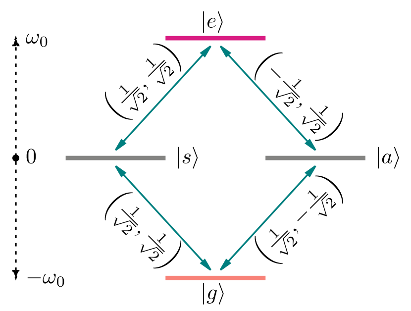
where $|g\rangle$ and $|e\rangle$ correspond to the ground and the excited states of the collective system, while $|s\rangle$ and $|a\rangle$ denote the symmetric and anti-symmetric maximally entangled Bell states. A pictorial representation of the different states and the associated energy levels of the two entangled detectors is illustrated in Fig. 1.

Refer to caption — Figure 1: An illustration of the energy levels corresponding to the eigen states of the two entangled detectors with two levels each. (We should mention that this figure has been taken from Ref. Picanço et al. (2020).) The contributions from the monopole moment for each transition have also been indicated in the figure.

In $(2+1)$ -dimensional Minkowski spacetime, the Hamiltonian of the massless, free scalar field is given by

H_{\mathrm{F}}=\frac{1}{2}\int{\rm d}^{2}{\bm{x}}\,\left[\dot{\Phi}^{2}(\tilde{x})+\left|\bm{\nabla}\Phi(\tilde{x})\right|^{2}\right],

(5)

where the overdot denotes differentiation with respect to the time coordinate, and $\bm{\nabla}$ denotes the spatial gradient. The interaction Hamiltonian describing the monopole detectors and the scalar field is assumed to be

H_{\mathrm{I}}=\sum_{j=1}^{2}\mu_{j}\,m_{j}(\tau_{j})\,\kappa_{j}(\tau_{j})\,\Phi[\tilde{x}_{j}(\tau_{j})],

(6)

where $\mu_{j}$ denotes the strengths of the individual coupling between the detectors and the scalar field, while $m_{j}(\tau_{j})$ and $\kappa_{j}(\tau_{j})$ denote the monopole operators of the detectors and the switching functions, respectively. For identical atomic detectors, the coupling strengths between the detectors and the scalar field can be assumed to be the same, i.e. we can set $\mu_{1}=\mu_{2}=\mu$ . In such a case, the time evolution operator can be expressed as

	$\displaystyle\hat{U}$	$\displaystyle=$	$\displaystyle\mathcal{T}\;\exp\,\biggl{\{}-i\,\mu\int_{-\infty}^{\infty}\,\biggl{[}\hat{m}_{1}(\tau_{1})\,\kappa_{1}(\tau_{1})\,\hat{\Phi}[\tilde{x}_{1}(\tau_{1})]\,{\rm d}\tau_{1}$		(7)
			$\displaystyle+\,\hat{m}_{2}(\tau_{2})\,\kappa_{2}(\tau_{2})\,\hat{\Phi}[\tilde{x}_{2}(\tau_{2})]\,{\rm d}\tau_{2}\biggr{]}\biggr{\}},$		(7)

where $\mathcal{T}$ implies time ordering. Let $|\omega\rangle$ be the collective initial state of the two detector system, and $|\bar{\omega}\rangle$ be the collective final state. Also, let the initial state of the scalar field be the Minkowski vacuum $|0_{{}_{\mathrm{M}}}\rangle$ , and let $|\Theta\rangle$ be the final state of the scalar field. Under these conditions, the transition amplitude from the initial state $|\omega,0_{{}_{\mathrm{M}}}\rangle$ to the final state $|\bar{\omega},\Theta\rangle$ at the first order (when expanded in the strength of the coupling constant $\mu$ ) in perturbation theory is given by

$\displaystyle\mathcal{A}_{\|\omega,0_{{}_{\mathrm{M}}}\rangle\to\|\bar{\omega},\Theta\rangle}\!\!$	$\displaystyle=$	$\displaystyle\!\!\langle\Theta,\bar{\omega}\|\hat{U}\|\omega,0_{{}_{\mathrm{M}}}\rangle$	(8)
	$\displaystyle\simeq$	$\displaystyle-i\,\mu\,\langle\Theta,\bar{\omega}\|\int_{-\infty}^{\infty}\,\biggl{[}\kappa_{1}\,\hat{m}_{1}\,\hat{\Phi}(\tilde{x}_{1})\,{\rm d}\tau_{1}$
		$\displaystyle+\,\kappa_{2}\,\hat{m}_{2}\,\hat{\Phi}(\tilde{x}_{2})\,{\rm d}\tau_{2}\biggr{]}\|\omega,0_{{}_{\mathrm{M}}}\rangle.$

Note that we shall be interested in examining the final state of the detectors. The total transition probability of the detectors can be arrived at from the above transition amplitude by summing over all the final states $\left\{|\Theta\rangle\right\}$ of the field. The total transition probability of the two detectors can be expressed as

	$\displaystyle\Gamma_{\|\omega\rangle\to\|\bar{\omega}\rangle}(\mathcal{E})$	$\displaystyle=$	$\displaystyle\sum_{\left\{\|\Theta\rangle\right\}}\mathcal{A}_{\|\omega,0_{{}_{\mathrm{M}}}\rangle\to\|\bar{\omega},\Theta\rangle}\,\mathcal{A}_{\|\omega,0_{{}_{\mathrm{M}}}\rangle\to\|\bar{\omega},\Theta\rangle}^{\ast}$		(9)
		$\displaystyle\simeq$	$\displaystyle\mu^{2}\sum_{j,l=1}^{2}m_{j}^{\bar{\omega}\omega\ast}\,m_{l}^{\bar{\omega}\omega}\,F_{jl}(\mathcal{E}),$		(9)

where $\mathcal{E}=E_{\bar{\omega}}-E_{\omega}$ , with $E_{\omega}$ and $E_{\bar{\omega}}$ denoting the energy eigen values associated with the states $|\omega\rangle$ and $|\bar{\omega}\rangle$ , and $m_{j}^{\bar{\omega}\omega}=\langle\bar{\omega}|\hat{m}_{j}(0)|\omega\rangle$ . As we shall discuss below, the quantities $F_{jl}(\mathcal{E})$ —which we shall refer to as the auto or the cross transition probabilities—depend on the trajectory of the detectors.

Meanwhile, let us understand the values that the quantity $m_{j}^{\bar{\omega}\omega}$ can take. We shall assume that the operator describing the monopole moment of the detectors is given by

\hat{m}_{j}(0)=|e_{j}\rangle\langle g_{j}|+|g_{j}\rangle\langle e_{j}|.

(10)

This expression for the monopole operators can be utilized to determine the contributions due to specific transitions between the collective initial and final states of the two detectors. For instance, it can be shown that the transition from the collective ground state $|g\rangle$ to the collective excited state $|e\rangle$ (or the other way around) of the entangled detectors is not possible since $m_{j}^{ge}=m_{j}^{eg}=0$ . Also, one finds that $m_{1}^{se}=m_{2}^{se}=1/\sqrt{2}$ and $m_{1}^{ae}=-m_{2}^{ae}=-1/\sqrt{2}$ , which denote the amplitudes for transitions between the symmetric and anti-symmetric Bell states (viz. $|s\rangle$ and $|a\rangle$ ) and the excited state of the detectors, respectively. Moreover, one can show that the amplitudes for the transitions from the collective ground state to the symmetric and anti-symmetric Bell states are given by $m_{1}^{gs}=m_{2}^{gs}=1/\sqrt{2}$ and $m_{1}^{ga}=-m_{2}^{ga}=1/\sqrt{2}$ . The energy levels associated with the different states of the two entangled detectors and the various possible transitions are illustrated diagrammatically in Fig. 1 (taken from Ref. Picanço et al. (2020)).

Let us now shift our attention to the transition probabilities $F_{jl}(\mathcal{E})$ in Eq. (9). The explicit form of the transition probabilities $F_{jl}(\mathcal{E})$ are found to be

	$\displaystyle F_{jl}(\mathcal{E})$	$\displaystyle=$	$\displaystyle\int_{-\infty}^{\infty}{\rm d}\tau_{l}^{\prime}\int_{-\infty}^{\infty}{\rm d}\tau_{j}\,\mathrm{e}^{-i\,\mathcal{E}\,(\tau_{j}-\tau_{l}^{\prime})}$		(11)
			$\displaystyle\times\,G_{jl}^{+}[\tilde{x}_{j}(\tau_{j}),\tilde{x}_{l}(\tau_{l}^{\prime})]\,\kappa_{j}(\tau_{j})\,\kappa_{l}(\tau_{l}^{\prime}),$		(11)

where the quantity $G_{jl}^{+}[\tilde{x}_{j}(\tau_{j}),\tilde{x}_{l}(\tau_{l}^{\prime})]$ denotes the positive frequency Wightman function evaluated along the trajectories of the detectors. The positive frequency Wightman function is defined as

G_{jl}^{+}[\tilde{x}_{j}(\tau_{j}),\tilde{x}_{l}(\tau_{l}^{\prime})]=\langle 0_{{}_{\mathrm{M}}}|\hat{\Phi}[\tilde{x}_{j}(\tau_{j})]\,\hat{\Phi}[\tilde{x}_{l}(\tau_{l}^{\prime})]|0_{{}_{\mathrm{M}}}\rangle.

(12)

In the following sections, we shall evaluate the transition probabilities of detectors that are in motion on circular trajectories in $(2+1)$ -dimensional Minkowski spacetime. We shall evaluate the responses of the detectors in the Minkowski vacuum as well as in a thermal bath. As we shall see, it proves to be convenient to work in terms of the polar coordinates to arrive at the Wightman function along the trajectories of the detectors when they are in circular motion.

III Response of a detector in circular motion

In this section, we shall derive the response of a single Unruh-DeWitt detector that is interacting with a scalar field. The results we obtain in this situation will prove to be helpful for understanding the results in the case of the two entangled detectors. Consider a massless and minimally coupled scalar field $\Phi$ that is described by the action

S[\Phi]=-\int{\rm d}^{3}x\,\sqrt{-g}\,\frac{1}{2}\,g^{\mu\nu}\,{\partial}_{\mu}\Phi\,{\partial}_{\nu}\Phi.

(13)

On varying the action, we can obtain the equation of motion of the scalar field to be

\Box\Phi=\frac{1}{\sqrt{-g}}\,{\partial}_{\mu}\left(\sqrt{-g}\,g^{\mu\nu}\,{\partial}_{\nu}\right)\Phi=0.

(14)

In order to examine the behavior of a rotating detector in Minkowski spacetime, it proves to be convenient to work in the polar coordinates so that, in $(2+1)$ -dimensions, the spacetime coordinates are given by $\tilde{x}=(t,\rho,\phi)$ . In these coordinates, the normal modes of the massless scalar field can be obtained to be

u_{qm}(\tilde{x})=\frac{1}{\sqrt{4\,\pi}}\,\mathrm{e}^{-i\,q\,t}\,J_{m}(q\,\rho)\,\mathrm{e}^{i\,m\,\phi},

(15)

where $0\leq q<\infty$ , $m$ is an integer, and $J_{n}(z)$ denotes the Bessel function of order $n$ . On quantization, the scalar field can be decomposed in terms of the above normal modes $u_{qm}(\tilde{x})$ as follows:

\hat{\Phi}(\tilde{x})=\int_{0}^{\infty}{\rm d}q\sum_{m=-\infty}^{\infty}\left[\hat{a}_{qm}\,u_{qm}(\tilde{x})+\hat{a}_{qm}^{\dagger}\,u_{qm}^{\ast}(\tilde{x})\right],

(16)

where $\hat{a}_{qm}$ and $\hat{a}_{qm}^{\dagger}$ are the creation and the annihilation operators which satisfy the following standard commutation relations:


$\displaystyle\left[\hat{a}_{qm},\hat{a}_{q^{\prime}m^{\prime}}\right]$	$\displaystyle=$	$\displaystyle\left[\hat{a}_{qm}^{\dagger},\hat{a}_{q^{\prime}m^{\prime}}^{{\dagger}}\right]=0,$	(17a)
$\displaystyle\left[\hat{a}_{qm},\hat{a}_{q^{\prime}m^{\prime}}^{{\dagger}}\right]$	$\displaystyle=$	$\displaystyle\delta^{(1)}(q-q^{\prime})\,\delta_{mm^{\prime}}.$	(17b)

In the case of a single detector, the transition probability (11) simplifies to be

	$\displaystyle F(\mathcal{E})$	$\displaystyle=$	$\displaystyle\int_{-\infty}^{\infty}{\rm d}\tau^{\prime}\int_{-\infty}^{\infty}{\rm d}\tau\,\mathrm{e}^{-i\,\mathcal{E}\,(\tau-\tau^{\prime})}$		(18)
			$\displaystyle\times\,G^{+}[\tilde{x}(\tau),\tilde{x}(\tau^{\prime})]\,\kappa(\tau)\,\kappa(\tau^{\prime}).$		(18)

In our discussion, we shall be interested in examining the response of detectors that are moving on circular trajectories. Also, we shall evaluate the response of the detectors in the Minkowski vacuum and in a thermal bath. We shall utilize the mode functions (15) in the polar coordinates to arrive at the Wightman function $G^{+}(\tilde{x},\tilde{x}^{\prime})$ in both these situations. One finds that, in these situations, the Wightman function along the trajectory of a detector in circular motion is invariant under the time translation in the proper time in the frame of the detector, i.e. $G^{+}[\tilde{x}(\tau),\tilde{x}(\tau^{\prime})]=G^{+}(\tau,\tau^{\prime})=G^{+}(u)$ , where $u=(\tau-\tau^{\prime})$ . It is well known that such a time translation invariance allows one to define the transition probability rate of the detector. Often, in these contexts, the Wightman function is first evaluated by summing over all the normal modes of the quantum field, before evaluating the transition probability rate of the detector. As we shall see, to arrive at the transition probability rate of the rotating detector, rather than explicitly evaluate the Wightman function, it proves to be convenient to first carry out the integral over the quantity $u$ , and then sum over the modes. In the following subsections, we shall evaluate the transition probability rate of a rotating detector that has been switched on for infinite as well as a finite time interval.

III.1 Detector switched on for infinite duration

Let us first consider the situation wherein the detector remains switched on for all times. In such a situation, the switching function $\kappa(\tau)$ reduces to unity.

III.1.1 Response in the Minkowski vacuum

Let us now evaluate the response of the rotating detector in the Minkowski vacuum. The Wightman function $G^{+}(\tilde{x},\tilde{x}^{\prime})$ associated with the massless scalar field in the Minkowski vacuum can be expressed as (in this regard, also see App. A)

$\displaystyle G^{+}(x,x^{\prime})$	$\displaystyle=$	$\displaystyle\langle 0_{{}_{\mathrm{M}}}\|\hat{\Phi}(\tilde{x})\,\hat{\Phi}(\tilde{x}^{\prime})\|0_{{}_{\mathrm{M}}}\rangle$	(19)
	$\displaystyle=$	$\displaystyle\int_{0}^{\infty}\frac{{\rm d}q}{4\,\pi}\,\sum_{m=-\infty}^{\infty}J_{m}(q\,\rho)\,J_{m}(q\,\rho^{\prime})$
		$\displaystyle\times\,\mathrm{e}^{-i\,q\,(t-t^{\prime})}\,\mathrm{e}^{i\,m\,(\phi-\phi^{\prime})},$

where we have made use of the fact that the Bessel functions $J_{n}(x)$ are real for integer values of $n$ and real arguments. In order to arrive at the response of the detector, we need to calculate the above Wightman function along the trajectory of the detector. Let us assume that the detector is moving along a circular trajectory with radius $\sigma$ , at a constant angular velocity $\Omega$ . If $\tau$ is the proper time in the frame of the detector, then the trajectory of the detector is given by (see, for example, Refs. Gutti et al. (2011); Picanço et al. (2020))

t=\gamma\,\tau,\quad\rho=\sigma,\quad\phi=\gamma\,\Omega\,\tau,

(20)

where $\gamma=1/\sqrt{1-v^{2}}$ is the Lorentz factor associated with the linear velocity $v=\sigma\,\Omega$ of the detector. Along such a trajectory, the Wightman function above reduces the following form:

G^{+}(u)=\int_{0}^{\infty}\frac{{\rm d}q}{4\,\pi}\,\sum_{m=-\infty}^{\infty}J_{m}^{2}(q\,\sigma)\,\mathrm{e}^{-i\,\gamma\,(q-m\,\Omega)\,u},

(21)

where, as we mentioned above, $u=(\tau-\tau^{\prime})$ . In such a situation, we can define the transition probability rate of the detector to be

R(\mathcal{E})=\int_{-\infty}^{\infty}{\rm d}u\,\mathrm{e}^{-i\,\mathcal{E}\,u}\,G^{+}(u).

(22)

On substituting the Wightman function (21) along the trajectory of the rotating detector in the above expression, we find that the transition probability rate can be expressed as

	$\displaystyle R(\bar{\mathcal{E}})$	$\displaystyle=$	$\displaystyle\sum_{m=-\infty}^{\infty}\,\int_{0}^{\infty}\frac{{\rm d}q}{2\,\gamma}\,J^{2}_{m}(q\,\sigma)\,\delta^{(1)}[q-(m-\bar{\mathcal{E}})\,\Omega]$		(23)
		$\displaystyle=$	$\displaystyle\frac{1}{2\,\gamma}\,\sum_{m\geq\bar{\mathcal{E}}}^{\infty}J^{2}_{m}\left[(m-\bar{\mathcal{E}})\,v\right],$		(23)

where we have introduced the dimensionless energy gap $\bar{\mathcal{E}}=\mathcal{E}/(\gamma\,\Omega)$ and, recall that, $v=\sigma\,\Omega$ is the linear velocity of the detector. Note that, since $q\in[0,\infty)$ , the Dirac delta function in the above expression leads to non-zero contributions only when $m\geq\bar{\mathcal{E}}$ , which is reflected in the lower limit of the sum in the final expression.

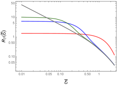
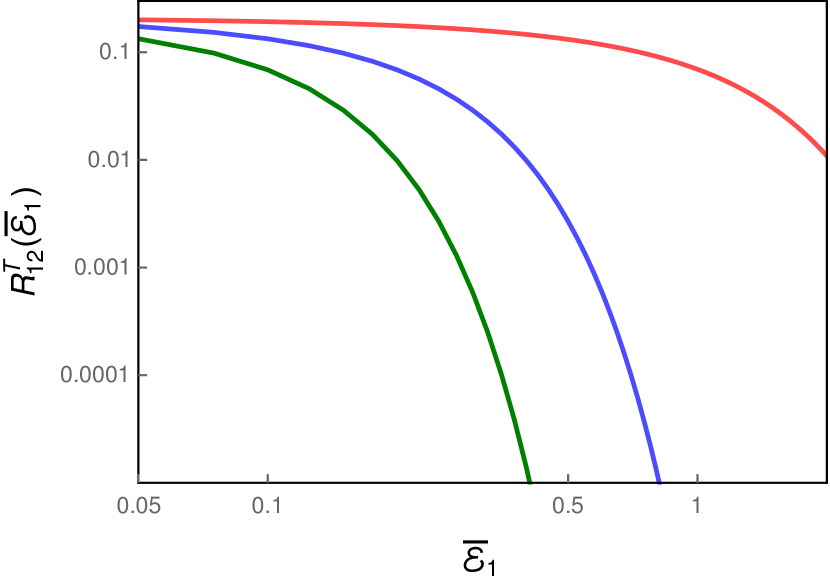
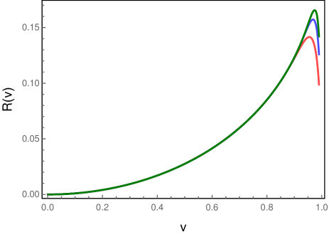
Evidently, the transition probability rate (23) of the detector in circular motion depends only on its linear velocity $v$ . The sum in the expression for the transition probability rate proves to be difficult to evaluate analytically. But, it converges quickly enough to be computed numerically. For a given value of $\bar{\mathcal{E}}$ , we find that the sum converges exponentially beyond a certain value of $m$ . For instance, we find that, when $\bar{\mathcal{E}}$ is chosen to be unity, for $v=(0.25,0.5,0.75)$ , the quantity $J^{2}_{m}\left[(m-\bar{\mathcal{E}})\,v\right]$ that appears in the sum characterizing the transition probability rate of the detector decreases at least as fast as $(\mathrm{e}^{-2.0\,m},\mathrm{e}^{-0.9\,m},\mathrm{e}^{-0.25\,m})$ , respectively, at suitably large $m$ . We should clarify that we have confirmed this behavior for adequately large values of $m$ , much beyond the values we sum over to arrive at the result. The rapid convergence of the sum allows us to easily calculate the transition probability rate of the rotating detector numerically by summing up to a finite value of $m$ (in this regard, also see, App. B). We have also ensured that, over the domain of $\bar{\mathcal{E}}$ we focus on, the contributions beyond the maximum value of $m$ we have worked with are insignificant. In Fig. 2, we have illustrated the transition probability rate of the detector as a function of the dimensionless energy gap $\bar{\mathcal{E}}$ for a few different values of the velocity.

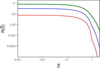
The figure suggests that, higher the velocity of the detector, higher is its transition probability rate. Moreover, for a given velocity, the transition probability of the detector is larger at smaller values of the energy gap such that $\bar{\mathcal{E}}\ll 1$ .

III.1.2 Response in a thermal bath

Let us now turn to evaluate the response of the detector in a thermal bath. We shall assume that the massless scalar field $\Phi$ of our interest is in equilibrium with a thermal bath maintained at the inverse temperature $\beta$ . We can utilize the decomposition (16) of the scalar field in terms of the normal modes (15) to arrive at the following expression for the Wightman function at a finite temperature (in this context, also see App. A):

$\displaystyle G^{+}_{\beta}(\tilde{x},\tilde{x}^{\prime})$	$\displaystyle=$	$\displaystyle\int_{0}^{\infty}\frac{{\rm d}q}{4\,\pi}\,\sum_{m=-\infty}^{\infty}J_{m}(q\,\rho)\,J_{m}(q\,\rho^{\prime})$	(24)
		$\displaystyle\times\,\biggl{\{}\frac{\mathrm{e}^{-i\,[q\,(t-t^{\prime})-m\,(\phi-\phi^{\prime})]}}{1-\mathrm{e}^{-\beta\,q}}$
		$\displaystyle+\,\frac{\mathrm{e}^{i\,[q\,(t-t^{\prime})-m\,(\phi-\phi^{\prime})]}}{\mathrm{e}^{\beta\,q}-1}\biggr{\}}.$

Along the trajectory (20) of the rotating detector, this finite temperature Wightman function too turns out to be invariant under translations in the proper time of the detector as in the Minkowski vacuum. We find that, in the frame of the rotating detector, the finite temperature Wightman function reduces to

	$\displaystyle G^{+}_{\beta}(u)$	$\displaystyle=$	$\displaystyle\int_{0}^{\infty}\frac{{\rm d}q}{4\,\pi}\,\sum_{m=-\infty}^{\infty}J^{2}_{m}(q\,\sigma)$		(25)
			$\displaystyle\times\,\left[\frac{\mathrm{e}^{-i\,\gamma\,(q-m\,\Omega)\,u}}{1-\mathrm{e}^{-\beta\,q}}+\frac{\mathrm{e}^{i\,\gamma\,(q-m\,\Omega)\,u}}{\mathrm{e}^{\beta\,q}-1}\right].\qquad$		(25)

Since the Wightman function depends only on the quantity $u$ , we can define a transition probability rate for the detector as in the Minkowski vacuum [cf. Eq. (22)]. The transition probability rate of the rotating detector at a finite temperature can be easily evaluated to be

$\displaystyle R(\bar{\mathcal{E}})$	$\displaystyle=$	$\displaystyle\sum_{m=-\infty}^{\infty}\,\int_{0}^{\infty}\frac{{\rm d}q}{2\,\gamma}\,J^{2}_{m}(q\,\sigma)\,\biggl{\{}\frac{\delta^{(1)}[q-(m-\bar{\mathcal{E}})\,\Omega]}{1-\mathrm{e}^{-\beta\,q}}$	(26)
		$\displaystyle+\,\frac{\delta^{(1)}[q-(m+\bar{\mathcal{E}})\,\Omega]}{\mathrm{e}^{\beta\,q}-1}\biggr{\}}$
	$\displaystyle=$	$\displaystyle\frac{1}{2\,\gamma}\,\biggl{\{}\sum_{m\geq\bar{\mathcal{E}}}^{\infty}\,\frac{J^{2}_{m}\left[(m-\bar{\mathcal{E}})\,v\right]}{1-\mathrm{e}^{-\bar{\beta}\,(m-\bar{\mathcal{E}})}}$
		$\displaystyle+\,\sum_{m\geq-\bar{\mathcal{E}}}^{\infty}\frac{J^{2}_{m}\left[(m+\bar{\mathcal{E}})\,v\right]}{\mathrm{e}^{\bar{\beta}\,(m+\bar{\mathcal{E}})}-1}\biggr{\}},$

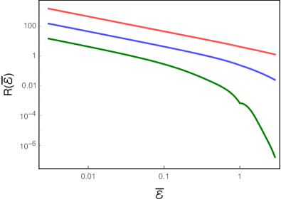
where $\bar{\beta}=\beta\,\Omega$ denotes the dimensionless inverse temperature of the bath. We had noted earlier that, the quantity $J^{2}_{m}\left[(m-\bar{\mathcal{E}})\,v\right]$ which appears in the sum characterizing the transition probability rate decreases exponentially at large $m$ . Though the sums in the above expression are again difficult to evaluate analytically, such a rapid convergence allows us to compute them numerically rather easily (again, in this regard, see, App. B). Actually, in the case of the second term, the exponential in the denominator also aids in a faster convergence of the sum. In Fig. 2, we have plotted the above transition probability rate of the detector for a fixed value of the velocity $v$ and a few different values of the dimensionless inverse temperature $\bar{\beta}$ . It should be clear from the figure that, larger the temperature (or, equivalently, smaller the value of $\bar{\beta}$ ), larger is the transition probability rate of the rotating detector.

At this stage, there is a technical point that we need to discuss. Actually, the finite temperature Wightman function (25) contains an infrared divergence. As $q\to 0$ , the functions $J_{m}^{2}(q\,\sigma)$ behave as $q^{2\,m}$ and, hence, the $m=0$ term in the Wightman function diverges logarithmically in this limit even for finite separation of the spacetime points. This behavior is a surprising and less known peculiarity of the thermal Green’s function in $(2+1)$ -dimensional Minkowski spacetime and, in fact, the divergence is absent at zero temperature [as can be easily checked with the Wightman function (21)]. Also, it can be readily shown that such an infrared divergence is not encountered in $(3+1)$ -dimensional Minkowski spacetime. We should point out that the infrared divergence occurs in addition to the ultraviolet divergence which arises at large $q$ . The ultraviolet divergence can, as usual, be regulated using the $(i\,\epsilon)$ -prescription. Note that, in arriving at the rate $R(\bar{\mathcal{E}})$ in Eq. (26), we chose to calculate the integral over $u$ first before evaluating the integral over $q$ . In the process, the infrared divergence is transferred to the $m=\pm\bar{\mathcal{E}}$ term in the sum, and it manifests itself only in the $\bar{\mathcal{E}}\to 0$ limit. But, since we have assumed that $\mathcal{E}>0$ , we do not actually encounter the divergence when evaluating the sum. In the following section, when we consider detectors which are switched on for a finite duration, we shall find that the divergence at the finite temperature cannot be circumvented in a similar manner. To handle the divergence, we shall adopt a procedure which allows us to reproduce the results in the different limits, viz. at zero temperature and when the detector is switched on for infinite duration.

There is another point that we need to clarify regarding the results illustrated in Fig. 2. Note that, in the case of results plotted at a finite temperature, the transition probability rate $R(\bar{\mathcal{E}})$ turns out to be more than unity for small values of $\bar{\mathcal{E}}$ . This may cause concern. But, it occurs due to the fact that we have dropped an overall factor of $|\mu|^{2}$ , where $\mu$ is the coupling constant that determines the strength of the interaction between the detector and the field [cf. Eq. (6)], when evaluating the transition probability rate. In order for the perturbative expansion of the time evolution operator in Eq. (7) to be valid, we require $\mu$ to be much smaller than unity. Evidently, for a suitably small value of $|\mu|^{2}$ , the transition probability rate will reduce to a value less than unity for all energies $\bar{\mathcal{E}}$ .

We will now show that the transition probability rate of the rotating detector in a thermal bath we have obtained above corresponds to the accumulation of different types of radiative processes that occur in the system. Let us introduce the quantities

\mathcal{N}_{r}(q,\bar{\mathcal{E}})=\frac{1}{2\,\gamma}\sum_{m=-\infty}^{\infty}J^{2}_{m}(q\,\sigma)\,\delta^{(1)}[q-(m-\bar{\mathcal{E}})\,\Omega]

(27)

and

\mathcal{N}_{\beta}(q)=\frac{1}{\mathrm{e}^{\beta\,q}-1}.

(28)

Since $(1-\mathrm{e}^{-x})^{-1}=1+(\mathrm{e}^{x}-1)^{-1}$ , in terms of the above quantities, we can re-express the first equality of Eq. (26) in the following form:

	$\displaystyle R(\bar{\mathcal{E}})$	$\displaystyle=$	$\displaystyle\underbrace{\int_{0}^{\infty}{\rm d}q\,\mathcal{N}_{r}(q,\bar{\mathcal{E}})}_{R_{1}(\bar{\mathcal{E}})}$		(29)
			$\displaystyle+\,\underbrace{\int_{0}^{\infty}{\rm d}q\,\mathcal{N}_{\beta}(q)\,\left[\mathcal{N}_{r}(q,\bar{\mathcal{E}})+\mathcal{N}_{r}(q,-\bar{\mathcal{E}})\right]}_{R_{2}(\bar{\mathcal{E}},\beta)}.\qquad$		(29)

In other words, we can express the transition probability rate of the rotating detector in a thermal bath as a sum of the two contributions $R_{1}(\bar{\mathcal{E}})$ and $R_{2}(\bar{\mathcal{E}},\beta)$ , which, as we shall soon discuss, can be attributed to different types of radiative processes. Note that the first term $R_{1}(\bar{\mathcal{E}})$ is only a function of $\bar{\mathcal{E}}$ and is independent of $\beta$ , whereas the second term $R_{2}(\bar{\mathcal{E}},\beta)$ is a function of both $\bar{\mathcal{E}}$ and $\beta$ . The fact that the term $R_{1}(\bar{\mathcal{E}})$ is the same as the first equality in Eq. (23) clearly suggests that it corresponds to the response of the rotating detector in the Minkowski vacuum. The contribution arises due to modes with the magnetic quantum numbers $m_{1}=(q/\Omega)+\bar{\mathcal{E}}$ for a given value of momentum $q$ . A contribution from the Minkowski vacuum can always be expected to occur and the contribution can be interpreted as arising due to the spontaneous excitation of the detector. The interesting aspect of the term $R_{2}(\bar{\mathcal{E}},\beta)$ is the appearance of the factor $\mathcal{N}_{\beta}(q)$ . The factor represents the distribution of scalar field modes with momentum $q$ and it reflects the fact that the scalar field is immersed in a thermal bath. Actually, the contribution $R_{2}(\bar{\mathcal{E}},\beta)$ consists of two parts. The first part involving $\mathcal{N}_{r}(q,\bar{\mathcal{E}})$ can be interpreted as the excitation of the rotating detector due to the thermal nature of the scalar field, with modes corresponding to the magnetic quantum number $m_{1}$ contributing to the transition probability rate of the detector. The second part involving $\mathcal{N}_{r}(q,-\bar{\mathcal{E}})$ too signifies the excitation of detector by the thermal character of the field, but with the contributions arising from modes with a different set of magnetic quantum number, viz. $\bar{m}_{1}=(q/\Omega)-\bar{\mathcal{E}}$ . Evidently, these latter two contributions can be attributed to the combined effects of both the circular motion of the detector as well as the thermal bath. Since these contributions are influenced by the presence of the thermal bath and vanish in its absence (i.e. when $\beta\to\infty$ ), these contributions can be interpreted as arising due to the stimulated excitation of the detector. Therefore, the overall response of the rotating detector in the thermal bath can be interpreted as arising due to the accumulation of three types of radiative process—two processes (spontaneous and stimulated excitation) to which the scalar field modes with the magnetic quantum number $m_{1}$ contribute and another process (stimulated excitation) which arises due to the contributions by the modes with quantum number $\bar{m}_{1}$ .

In this regard, it may be pointed out that a similar interpretation has also been suggested earlier for the response of a uniformly accelerated detector in a thermal bath (see Refs. Kolekar and Padmanabhan (2015); Kolekar (2014); Kolekar and Padmanabhan (2014)). However, we observe a noticeable difference between the transition probability rates of accelerated detectors and our present system. In the accelerated case, the second term in Eq. (29), which we had interpreted as due to stimulated excitation, has a simpler structure. It is composed of a purely thermal contribution and an excitation due to the acceleration effects stimulated by the thermal bath. Therefore, for an accelerated detector in a thermal bath, there are two independent, spontaneous excitations—one is due to the acceleration (known as the Unruh effect), and the other is purely due to the thermal bath; apart from stimulated excitation, which is influenced by the thermal background. Whereas, in the present study, we do not find any contribution due to the thermal bath that is independent of rotation. This aspect of the transition probability rates of rotating detectors in a thermal bath provides a signature distinct from the case of accelerated detectors.

III.2 Detector switched on for a finite duration

Let us now consider the case wherein the detectors are assumed to be switched on for a finite time interval, say, $T$ . We shall consider the switching functions $\kappa(\tau)$ to be of the following Gaussian form Sriramkumar and Padmanabhan (1996):

\kappa(\tau)=\mathrm{exp}\,\left(-\frac{\tau^{2}}{T^{2}}\right),

(30)

where, evidently, $T$ denotes the duration for which the detector remains effectively switched on. In the presence of such a switching function, the transition probability of the detector is given by [cf. Eq. (11)]

	$\displaystyle F_{T}(\mathcal{E})$	$\displaystyle=$	$\displaystyle\int_{-\infty}^{\infty}{\rm d}\tau^{\prime}\int_{-\infty}^{\infty}{\rm d}\tau\,\mathrm{e}^{-i\,\mathcal{E}\,(\tau-\tau^{\prime})}\,G^{+}(\tau,\tau^{\prime})$		(31)
			$\displaystyle\times\,\mathrm{exp}\,\left[-(\tau^{2}+{\tau^{\prime}}^{2})/T^{2}\right].$		(31)

On changing variables to $u=(\tau-\tau^{\prime})$ and $v=(\tau+\tau^{\prime})$ , the integral can be expressed as

	$\displaystyle F_{T}(\mathcal{E})$	$\displaystyle=$	$\displaystyle\int_{-\infty}^{\infty}\frac{{\rm d}v}{2}\,\mathrm{e}^{-v^{2}/(2\,T^{2})}$		(32)
			$\displaystyle\times\,\int_{-\infty}^{\infty}{\rm d}u\,\mathrm{e}^{-i\,\mathcal{E}\,u}\,G^{+}(u,v)\,\mathrm{e}^{-u^{2}/(2\,T^{2})}.\qquad$		(32)

In cases wherein the Wightman function is invariant under time translations in the frame of the detector, i.e. when $G^{+}(\tau,\tau^{\prime})=G^{+}(u)$ —as in the case of the rotating detector [cf. Eqs. (21) and (25)]—we can carry out the Gaussian integral over $v$ to define the transition probability rate of the detector as follows:

	$\displaystyle R_{T}(\mathcal{E})$	$\displaystyle=$	$\displaystyle\frac{F_{T}(\mathcal{E})}{\sqrt{(\pi/2)}\;T}$		(33)
		$\displaystyle=$	$\displaystyle\int_{-\infty}^{\infty}{\rm d}u\,\mathrm{e}^{-i\,\mathcal{E}\,u}\,G^{+}(u)\,\mathrm{e}^{-u^{2}/(2\,T^{2})}.\qquad$		(33)

Note that, as required, $R_{T}(\mathcal{E})\to R(\mathcal{E})$ [cf. Eq. (22)] when $T\to\infty$ . We shall now utilize the above expression to evaluate the finite time response of the rotating detector in the Minkowski vacuum and in a thermal bath.

III.2.1 Response in the Minkowski vacuum

On utilizing the expression (21) for the Wightman function in the Minkowski vacuum along the circular trajectory, the transition probability rate of the detector that is switched on for a finite time interval $T$ can be expressed as

	$\displaystyle R_{T}(\mathcal{E})$	$\displaystyle=$	$\displaystyle\int_{0}^{\infty}\frac{{\rm d}q}{4\,\pi}\,\sum_{m=-\infty}^{\infty}J^{2}_{m}(q\,\sigma)$		(34)
			$\displaystyle\times\,\int_{-\infty}^{\infty}{\rm d}u\,\mathrm{e}^{-i\,\left[\mathcal{E}+\gamma\,(q-m\,\Omega)\right]\,u}\,\mathrm{e}^{-u^{2}/(2\,T^{2})}.\qquad\;\;$		(34)

The Gaussian integral over $u$ can be calculated easily to arrive at

	$\displaystyle R_{T}(\mathcal{E})$	$\displaystyle=$	$\displaystyle\sqrt{2\,\pi}\;T\,\sum_{m=-\infty}^{\infty}\,\int_{0}^{\infty}\frac{{\rm d}q}{4\,\pi}\,J^{2}_{m}(q\,\sigma)$		(35)
			$\displaystyle\times\,\mathrm{e}^{-\left[\mathcal{E}+\gamma\,(q-m\,\Omega)\right]^{2}\,T^{2}/2}.\qquad$		(35)

Recall that the Dirac delta function can be represented in terms of the Gaussian function as follows:

\delta^{(1)}(z)=\lim_{\alpha\to\infty}\frac{\alpha}{\sqrt{2\,\pi}}\,\mathrm{e}^{-\alpha^{2}\,z^{2}/2}.

(36)

Therefore, in the limit $T\to\infty$ , the expression (35) for the finite time response rate of the detector reduces to the result (23) for detectors that remain switched on for infinite time (with the identification of $\alpha=\gamma\,T$ ), as required. Upon noting that $J_{n}^{2}(x)=J_{-n}^{2}(x)$ for integer $n$ and real $x$ and setting $q=x\,\Omega$ , the integral (35) can be expressed as

	$\displaystyle R_{T}(\bar{\mathcal{E}})$	$\displaystyle=$	$\displaystyle\frac{\sqrt{2\,\pi}\;\bar{T}}{4\,\pi\gamma}\,\mathrm{e}^{-\bar{\mathcal{E}}^{2}\,\bar{T}^{2}/2}\,\Biggl{\{}\int_{0}^{\infty}{\rm d}x\,J^{2}_{0}(x\,v)\,\mathrm{e}^{-\left[(x^{2}/2)+x\,\bar{\mathcal{E}}\right]\,\bar{T}^{2}}\,$		(37)
			$\displaystyle+\,2\,\sum_{m=1}^{\infty}\,\mathrm{e}^{-m^{2}\,\bar{T}^{2}/2}\int_{0}^{\infty}{\rm d}x\,J^{2}_{m}(x\,v)\,\mathrm{e}^{-\left[(x^{2}/2)+x\,\bar{\mathcal{E}}\right]\,\bar{T}^{2}}\,\mathrm{cosh}\left[m\,(x+\bar{\mathcal{E}})\,\bar{T}^{2}\right]\Biggr{\}},$		(37)

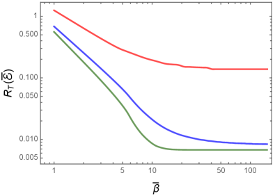
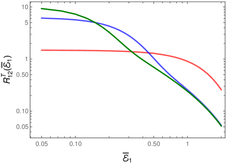
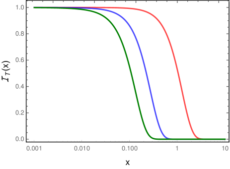
where we have defined the dimensionless time interval $\bar{T}=\gamma\,\Omega\,T$ . The above integrals and sum seem difficult to evaluate analytically, but they can be computed numerically. We find that the functions $J_{m}^{2}(x\,v)$ that appear in the integrands behave as $x^{2\,m}$ when $x\to 0$ , and as $x^{-1}$ when $x\to\infty$ (see, for instance, Refs. Watson (2015); Olver ). Note that the factors $\mathrm{e}^{-[(x^{2}/2)+x\,\bar{\mathcal{E}}]\,\bar{T}^{2}}$ and $\mathrm{cosh}\left[m\,(x+\bar{\mathcal{E}})\,\bar{T}^{2}\right]$ reduce to constants as $x\to 0$ . As a result, the integrals are well behaved at small $x$ . Moreover, at large $x$ , the integrals over $x$ are dominated by the factor $\mathrm{e}^{-x^{2}\,\bar{T}^{2}/2}$ , and hence converge quickly (in this regard, also see App. C). We evaluate the integrals up to a suitably large value of $x$ and then carry out the sum involved. In fact, we find that, because of the factor $\mathrm{e}^{-m^{2}\,\bar{T}^{2}/2}$ , the sum too converges extremely quickly. In Fig. 3, we have plotted the transition probability rate of the detector in circular motion for a given value of the velocity $v$ and a few different values of the dimensionless time interval $\bar{T}$ .

Note that, when $\bar{T}$ is made larger, as expected, the transition probability rate approaches the response rate of the detector that remains switched on forever. Interestingly, for a given energy $\bar{\mathcal{E}}$ and velocity $v$ , the transition probability rate of a detector that is switched on for a shorter duration is higher. However, this seems to occur up to a specific value of $\bar{\mathcal{E}}$ . At sufficiently large values of $\bar{\mathcal{E}}$ and $\bar{T}$ , the transition rate $R_{T}(\bar{\mathcal{E}})$ decreases, and all the curves corresponding to different values of $\bar{T}$ merge with the transition probability rate of the detector that remains switched on forever.

III.2.2 Response in a thermal bath

Let us now evaluate the finite time response of the detector in circular motion when it is immersed in a thermal bath. As earlier, we shall consider Gaussian switching functions [cf. Eq. (30)]. On substituting the Wightman function at a finite temperature along the trajectory of the rotating detector [cf. Eq. (25)] in the expression (33) that governs the transition probability rate of the detector, we obtain that

$\displaystyle R_{T}(\mathcal{E})$	$\displaystyle=$	$\displaystyle\int_{0}^{\infty}\frac{{\rm d}q}{4\,\pi}\,\sum_{m=-\infty}^{\infty}J^{2}_{m}(q\,\sigma)$	(38)
		$\displaystyle\times\int_{-\infty}^{\infty}{\rm d}u\,\biggl{\{}\frac{\mathrm{e}^{-i\,\left[\mathcal{E}+\gamma\,(q-m\,\Omega)\right]\,u}\,\mathrm{e}^{-u^{2}/(2\,T^{2})}}{1-\mathrm{e}^{-\beta\,q}}$
		$\displaystyle+\,\frac{\mathrm{e}^{-i\,\left[\mathcal{E}-\gamma\,(q-m\,\Omega)\right]\,u}\,\mathrm{e}^{-u^{2}/(2\,T^{2})}}{\mathrm{e}^{\beta\,q}-1}\biggr{\}}.$

Upon carrying out the Gaussian integral over $u$ , we arrive at

$\displaystyle R_{T}(\mathcal{E})$	$\displaystyle=$	$\displaystyle\sqrt{2\,\pi}\,T\,\int_{0}^{\infty}\frac{{\rm d}q}{4\,\pi}\,\sum_{m=-\infty}^{\infty}J^{2}_{m}(q\,\sigma)$	(39)
		$\displaystyle\times\,\biggl{\{}\frac{\mathrm{e}^{-\left[\mathcal{E}+\gamma\,(q-m\,\Omega)\right]^{2}\,T^{2}/2}}{1-\mathrm{e}^{-\beta\,q}}$
		$\displaystyle+\,\frac{\mathrm{e}^{-\left[\mathcal{E}-\gamma\,(q-m\,\Omega)\right]^{2}\,T^{2}/2}}{\mathrm{e}^{\beta\,q}-1}\biggr{\}}.$

One can further simplify this expression to eventually obtain that

$\displaystyle R_{T}(\bar{\mathcal{E}})$	$\displaystyle=$	$\displaystyle\frac{\sqrt{2\,\pi}\,\bar{T}}{4\,\pi\gamma}\,\mathrm{e}^{-\bar{\mathcal{E}}^{2}\,\bar{T}^{2}/2}\,\Biggl{\{}\int_{0}^{\infty}{\rm d}x\,J^{2}_{0}(x\,v)\,\Biggl{[}\frac{\mathrm{e}^{-\left[(x^{2}/2)+x\,\bar{\mathcal{E}}\right]\,\bar{T}^{2}}}{1-\mathrm{e}^{-\bar{\beta}\,x}}+\frac{\mathrm{e}^{-\left[(x^{2}/2)-x\,\bar{\mathcal{E}}\right]\,\bar{T}^{2}}}{\mathrm{e}^{\bar{\beta}\,x}-1}\Biggr{]}$	(40)
		$\displaystyle+\,2\,\sum_{m=1}^{\infty}\,\mathrm{e}^{-m^{2}\,\bar{T}^{2}/2}\int_{0}^{\infty}{\rm d}x\,J^{2}_{m}(x\,v)\,\Biggl{[}\frac{\mathrm{e}^{-\left[(x^{2}/2)+x\,\bar{\mathcal{E}}\right]\,\bar{T}^{2}}}{1-\mathrm{e}^{-\bar{\beta}\,x}}\,\mathrm{cosh}\left[m\,(x+\bar{\mathcal{E}})\,\bar{T}^{2}\right]$
		$\displaystyle+\,\frac{\mathrm{e}^{-\left[(x^{2}/2)-x\,\bar{\mathcal{E}}\right]\,\bar{T}^{2}}}{\mathrm{e}^{\bar{\beta}\,x}-1}\,\mathrm{cosh}\left[m\,(x-\bar{\mathcal{E}})\,\bar{T}^{2}\right]\Biggr{]}\Biggr{\}}.$

Recall that the functions $J_{m}^{2}(x\,v)$ behave as $x^{2\,m}$ when $x\to 0$ . Also, as we pointed out, the factors $\mathrm{e}^{-[(x^{2}/2)+x\,\bar{\mathcal{E}}]\,\bar{T}^{2}}$ and $\mathrm{cosh}\left[m\,(x+\bar{\mathcal{E}})\,\bar{T}^{2}\right]$ reduce to constants when $x\to 0$ . Moreover, note that the functions $(1-\mathrm{e}^{-\bar{\beta}\,x})$ and $(\mathrm{e}^{\bar{\beta}\,x}-1)$ behave as $x$ when $x\to 0$ . Therefore, in the $m=0$ term, as $x\to 0$ , the integrand in the above expression for $R_{T}(\bar{\mathcal{E}})$ behaves as $x^{-1}$ and the integration over $x$ leads to a logarithmic divergence as $x\to 0$ . This is the infrared divergence at the finite temperature which we had discussed earlier. In contrast to the case wherein the detectors are switched on forever, it proves to be more involved to handle the divergence when the detectors are switched on for a finite duration. We shall regulate the divergence using a procedure which ensures that we recover the results we have already obtained in the limits $\bar{T}\to\infty$ and $\bar{\beta}\to\infty$ . In order to avoid a long digression, we have discussed the procedure in App. E. Once we have tackled the divergence, the remaining terms can be evaluated without any difficulty. As in the earlier cases, we have evaluated the integrals and sum in Eq. (40) numerically to arrive at the response of the detector. We had pointed out that, even in the Minkowski vacuum, the integrals at large $x$ and the sum at large $m$ are dominated by the factors $\mathrm{e}^{-x^{2}\,\bar{T}^{2}/2}$ and $\mathrm{e}^{-m^{2}\,\bar{T}^{2}/2}$ , respectively. Hence, they converge very quickly, making it convenient to compute them numerically. In the finite temperature case of our interest, additionally, the contribution due to the exponential factor in the denominator in the final term leads to a more rapid convergence of the integral. We have checked that the results are robust against increasing the upper limits of the integral over $x$ and the sum over $m$ .

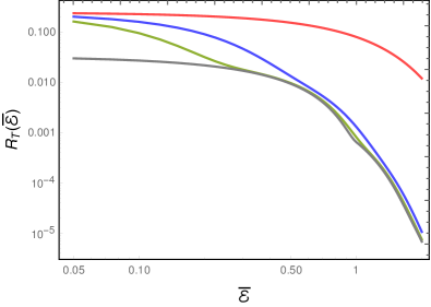
In Fig. 3, we have plotted the transition probability rate of the detector in circular motion and is immersed in a thermal bath for different values of the time interval $\bar{T}$ for which the detector remains effectively switched on, assuming a given velocity $v$ and inverse temperature $\beta$ .

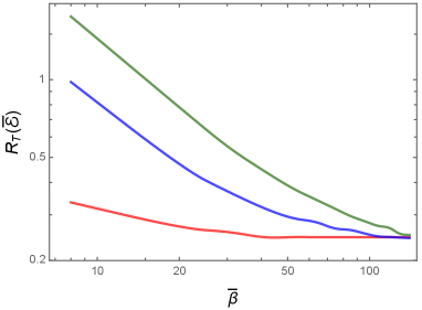
In contrast to the response in the Minkowski vacuum, we find that, at a finite temperature, the transition probability rate of the detector is lower at lower energies, when the detector is switched on for a shorter duration. It is only at high enough energies $\bar{\mathcal{E}}$ that the response is higher when $\bar{T}$ is made smaller. This point should also be clear from Fig. 4 wherein we have plotted the transition probability rate of the detector as a function of the dimensionless inverse temperature $\bar{\beta}$ for different values of $\bar{\mathcal{E}}$ and $\bar{T}$ .

We should point out here that, in the limit $\bar{\beta}\to\infty$ , the quantities $[1-\mathrm{exp}\,({-\bar{\beta}\,x})]^{-1}$ and $[\mathrm{exp}\,({\bar{\beta}\,x})-1]^{-1}$ in Eq. (40) reduce to unity and zero, respectively. Note that the limit $\bar{\beta}\to\infty$ implies a vanishing temperature for the thermal bath and hence corresponds to the Minkowski vacuum. In such a case, the transition probability rates (26) and (40) reduce to the corresponding results for the Minkowski vacuum, viz. Eqs. (23) and (37), as required. Moreover, recall that, earlier, in Eq. (29), we had expressed the transition probability rate of the rotating detector as a sum of different contributions arising due to spontaneous and stimulated excitations. We should point out here that the transition probability rate of the rotating detector which has been switched on for a finite time interval can also be expressed in a similar fashion.

IV Radiative processes of entangled detectors in circular motion

Having discussed the response of individual Unruh-DeWitt detectors, let us now turn to examine the responses of two entangled detectors that are moving on circular trajectories.

IV.1 Detectors switched on for infinite duration

As we have done earlier, let us first discuss the case wherein the detectors are switched on forever, before going to study the situations wherein the detectors are switched on for a finite time interval.

IV.1.1 Response in the Minkowski vacuum

Consider two detectors that are moving along the circular trajectories $\tilde{x}_{j}=(\gamma_{j}\,\tau_{j},\sigma_{j},\gamma_{j}\,\Omega_{j}\,\tau_{j})$ and $\tilde{x}_{l}=(\gamma_{l}\,\tau_{l},\sigma_{l},\gamma_{l}\,\Omega_{l}\,\tau_{l})$ , with $v_{j(l)}=\sigma_{j(l)}\,\Omega_{j(l))}$ and $\gamma_{j(l)}=1/\sqrt{1-v_{j(l)}^{2}}$ . The circular trajectories of the two detectors are, in general, assumed to be independent. On utilizing the mode decomposition (16) of the scalar field, the positive frequency Wightman function in the Minkowski vacuum which connects two spacetime points corresponding to two such detectors in circular motion can be obtained to be

$\displaystyle G^{+}_{jl}\left[x_{j}(\tau_{j}),x_{l}(\tau^{\prime}_{l})\right]$	$\displaystyle=$	$\displaystyle\int_{0}^{\infty}\frac{{\rm d}q}{4\,\pi}\sum_{m=-\infty}^{\infty}J_{m}(q\,\sigma_{j})\,J_{m}(q\,\sigma_{l})$	(41)
		$\displaystyle\times\,\mathrm{e}^{-i\,q\,(\gamma_{j}\,\tau_{j}-\gamma_{l}\,\tau^{\prime}_{l})}$
		$\displaystyle\times\,\mathrm{e}^{i\,m\,(\gamma_{j}\,\Omega_{j}\,\tau_{j}-\gamma_{l}\,\Omega_{l}\,\tau^{\prime}_{l})}.$

We can arrive at the total transition probability (9) corresponding to the entangled detectors by evaluating the auto and cross transition probabilities $F_{jl}(\mathcal{E})$ defined in Eq. (11).

To evaluate the auto and cross transition probabilities, let us consider the change of variables $\bar{u}=\tau_{j}-\tau^{\prime}_{l}$ and $\bar{v}=\tau_{j}+\tau^{\prime}_{l}$ . In terms of these new variables, for the case of detectors that are switched on forever, i.e. when $\kappa_{j}(\tau_{j})=\kappa_{l}(\tau_{l})=1$ , the transition probabilities $F_{jl}(\mathcal{E})$ can be expressed as

F_{jl}(\mathcal{E})=\int_{-\infty}^{\infty}\frac{{\rm d}\bar{v}}{2}\,\int_{-\infty}^{\infty}{\rm d}\bar{u}\,\mathrm{e}^{-i\,\mathcal{E}\,\bar{u}}\,G^{+}_{jl}(\bar{u},\bar{v}).

(42)

Upon using the inverse transformations $\tau_{j}=(\bar{v}+\bar{u})/2$ and $\tau^{\prime}_{l}=(\bar{v}-\bar{u})/2$ in the expression (41), we obtain the Wightman function $G^{+}_{jl}(\bar{u},\bar{v})$ for the two detectors moving on circular trajectories to be

	$\displaystyle G^{+}_{jl}(\bar{u},\bar{v})$	$\displaystyle=$	$\displaystyle\int_{0}^{\infty}\frac{{\rm d}q}{4\,\pi}\sum_{m=-\infty}^{\infty}J_{m}(q\,\sigma_{j})\,J_{m}(q\,\sigma_{l})$		(43)
			$\displaystyle\times\,\mathrm{e}^{-i\,[\alpha_{1}(q)\,\bar{v}+\alpha_{2}(q)\,\bar{u}]/2},$		(43)

where the quantities $\alpha_{1}(q)$ and $\alpha_{2}(q)$ are given by


$\displaystyle\alpha_{1}(q)$	$\displaystyle=$	$\displaystyle q\,(\gamma_{j}-\gamma_{l})-m\,(\gamma_{j}\,\Omega_{j}-\gamma_{l}\,\Omega_{l}),$	(44a)
$\displaystyle\alpha_{2}(q)$	$\displaystyle=$	$\displaystyle q\,(\gamma_{j}+\gamma_{l})-m\,(\gamma_{j}\,\Omega_{j}+\gamma_{l}\,\Omega_{l}).$	(44b)

On carrying the integral over $\bar{u}$ , we obtain the transition probability $F_{jl}(\mathcal{E})$ to be

$\displaystyle F_{jl}(\mathcal{E})$	$\displaystyle=$	$\displaystyle\int_{0}^{\infty}\frac{{\rm d}q}{2}\sum_{m=-\infty}^{\infty}J_{m}(q\,\sigma_{j})\,J_{m}(q\,\sigma_{l})$	(45)
		$\displaystyle\times\,\delta^{(1)}\left[\mathcal{E}+\frac{\alpha_{2}(q)}{2}\right]\,\int_{-\infty}^{\infty}\frac{{\rm d}\bar{v}}{2}\,\mathrm{e}^{-i\,\alpha_{1}(q)\,\bar{v}/2}$
	$\displaystyle=$	$\displaystyle\frac{1}{\gamma_{j}+\gamma_{l}}\,\sum_{m\geq\hat{\mathcal{E}}}^{\infty}J_{m}(q_{0}\,\sigma_{j})\,J_{m}(q_{0}\,\sigma_{l})~{}$
		$\displaystyle\times\,\int_{-\infty}^{\infty}\frac{{\rm d}\bar{v}}{2}\,\mathrm{e}^{-i\,\alpha_{1}(q_{0})\,\bar{v}/2},$

where the quantity $q_{0}$ is defined as

q_{0}=\frac{(m-\hat{\mathcal{E}})}{\gamma_{j}+\gamma_{l}}\,(\gamma_{j}\,\Omega_{j}+\gamma_{l}\,\Omega_{l})

(46)

with $\hat{\mathcal{E}}$ being given by

\hat{\mathcal{E}}=\frac{2\,\mathcal{E}}{\gamma_{j}\,\Omega_{j}+\gamma_{l}\,\Omega_{l}}.

(47)

We should point out that the condition $m\geq\hat{\mathcal{E}}$ arises since $q_{0}\geq 0$ . Let us now explicitly evaluate the transition probabilities $F_{jl}(\mathcal{E})$ for the cases $j=l$ and $j\neq l$ .

When $j=l$ , the trajectories correspond to the same detector so that we have $\gamma_{j}=\gamma_{l}$ and $\Omega_{j}=\Omega_{l}$ , which lead to $\alpha_{1}(q_{0})=0$ . In such a case, the expression (45) reduces to the transition probability of a single detector. We can also define the corresponding transition probability rate, say, $R_{jj}(\mathcal{E})$ , by dividing the quantity $F_{jj}(\mathcal{E})$ in Eq. (45) by the integral over $\bar{v}$ [cf. Eq. (22)]. Since, $\hat{\mathcal{E}}=\mathcal{E}/(\gamma_{j}\,\Omega_{j})=\bar{\mathcal{E}}_{j}$ and $q_{0}=(m-\bar{\mathcal{E}}_{j})\,\Omega_{j}$ when $j=l$ , we obtain the transition probability rate of the detector to be

R_{jj}(\bar{\mathcal{E}}_{j})=\frac{1}{2\,\gamma_{j}}\,\sum_{m\geq\bar{\mathcal{E}}_{j}}^{\infty}J^{2}_{m}\left[(m-\bar{\mathcal{E}}_{j})\,v_{j}\right],

(48)

where, as we mentioned before, the condition $m\geq\bar{\mathcal{E}}_{j}$ arises because $q_{0}\geq 0$ . This is exactly the result we had obtained earlier when we had considered the response of a single detector [cf. Eq. (23)]. When $j=1$ , the transition probability rate $R_{11}(\bar{\mathcal{E}}_{1})$ is given by the expression (23), with $(v,\gamma,\bar{\mathcal{E}}$ ) replaced by $(v_{1},\gamma_{1},\bar{\mathcal{E}}_{1})$ . If we define the dimensionless parameters $\bar{\Omega}=\Omega_{2}/\Omega_{1}$ and $\bar{\gamma}=\gamma_{2}/\gamma_{1}$ , then the transition probability $R_{22}(\bar{\mathcal{E}}_{1})$ can be expressed as

R_{22}(\bar{\mathcal{E}}_{1})=\frac{1}{2\,\gamma_{2}}\,\sum_{m\geq\bar{\mathcal{E}}_{1}/(\bar{\gamma}\,\bar{\Omega})}^{\infty}J^{2}_{m}\left[\left(m-\frac{\bar{\mathcal{E}}_{1}}{\bar{\gamma}\,\bar{\Omega}}\right)\,v_{2}\right].

(49)

Let us now consider the case wherein $j\neq l$ . When $j\neq l$ , the integral over $\bar{v}$ in Eq. (45) results in a delta function of the form $\delta^{(1)}[\alpha_{1}(q_{0})]$ , which can be utilized to define the transition probability rate. Also, the delta function leads to an additional constraint on $m$ . For the transition probability rate $R_{jl}(\mathcal{E})$ to be non-zero, other than the condition $m\geq\hat{\mathcal{E}}$ , we also require that

m=m_{0}=\frac{(\gamma_{l}-\gamma_{j})\,\mathcal{E}}{\gamma_{j}\,\gamma_{l}\,(\Omega_{j}-\Omega_{l})}.

(50)

In other words, the contribution to the transition probability rate arises due to only one term in the sum over $m$ , leading to

\displaystyle R_{jl}(\hat{\mathcal{E}})=\frac{1}{(\gamma_{j}+\gamma_{l})}\,J_{m_{0}}(q_{0}\,\sigma_{j})\,J_{m_{0}}(q_{0}\,\sigma_{l}),

(51)

and we should stress that this result is true only when $j\neq l$ . However, since $m_{0}$ has to be an integer, the relation (50) implies that it is only for some specific values of the parameters of the system that the transition probability rates $R_{12}(\mathcal{E})$ and $R_{21}(\mathcal{E})$ contribute to the radiative process. In terms of the dimensionless parameters $\bar{\gamma}$ and $\bar{\Omega}$ , we can express the transition probability rate $R_{12}(\bar{\mathcal{E}}_{1})$ as follows:

$\displaystyle R_{12}(\bar{\mathcal{E}}_{1})$	$\displaystyle=$	$\displaystyle\frac{1}{(\gamma_{1}+\gamma_{2})}\,J_{m_{0}}\left[(m_{0}-\hat{\mathcal{E}})\,\frac{(1+\bar{\gamma}\,\bar{\Omega})}{(1+\bar{\gamma})}\,v_{1}\right]$	(52)
		$\displaystyle\times\,J_{m_{0}}\left[(m_{0}-\hat{\mathcal{E}})\,\frac{(1+\bar{\gamma}\,\bar{\Omega})}{(1+\bar{\gamma})\,\bar{\Omega}}\,v_{2}\right]$
	$\displaystyle=$	$\displaystyle R_{21}(\bar{\mathcal{E}}_{1})$

with $\hat{\mathcal{E}}$ and $m_{0}$ being given by

	$\displaystyle\hat{\mathcal{E}}$	$\displaystyle=$	$\displaystyle\frac{2\,\mathcal{E}}{\gamma_{1}\,\Omega_{1}+\gamma_{2}\,\Omega_{2}}=\frac{2\,\bar{\mathcal{E}}_{1}}{1+\bar{\gamma}\,\bar{\Omega}},$
	$\displaystyle m_{0}$	$\displaystyle=$	$\displaystyle\frac{(\gamma_{2}-\gamma_{1})\,\mathcal{E}}{\gamma_{1}\,\gamma_{2}\,(\Omega_{1}\,-\Omega_{2})}=\frac{(1-1/\bar{\gamma})\,\bar{\mathcal{E}}_{1}}{1-\bar{\Omega}}.$		(53)

Let us now understand if the transition probability rate $R_{12}(\bar{\mathcal{E}}_{1})$ can be non-zero for values of the parameters describing the trajectories of the two detectors, viz. $(\Omega_{1},\gamma_{1})$ and $(\Omega_{2},\gamma_{2})$ , that we shall focus on. First, consider the case wherein $\gamma_{1}\neq\gamma_{2}$ , while $(\Omega_{1}-\Omega_{2})\to 0^{+}$ . In such a situation, $m_{0}\to\infty$ as $\Omega_{1}\to\Omega_{2}$ , and the required condition $m_{0}\geq\hat{\mathcal{E}}$ will indeed be satisfied. However, we find that, as $m\to\infty$ , the function $J_{m}(z)$ goes to zero (in this context, see Refs. Watson (2015); Olver ). This implies that the transition probability rate $R_{12}(\mathcal{E})$ vanishes. Second, when $\gamma_{1}=\gamma_{2}$ , we require $\Omega_{1}\neq\Omega_{2}$ so that they correspond to different trajectories for the two detectors. In such a situation, $m_{0}=0$ . However, since $\hat{\mathcal{E}}>0$ , the condition $m_{0}\geq\hat{\mathcal{E}}$ cannot be satisfied leading to a vanishing $R_{12}(\bar{\mathcal{E}}_{1})$ . Hence, in these situations, the complete transition probability rate of the two entangled detectors will be solely determined by the rates $R_{11}(\bar{\mathcal{E}}_{1})$ and $R_{22}(\bar{\mathcal{E}}_{1})$ of the individual detectors. Naturally, constructive or destructive effects due to the cross transition probability rates $R_{12}(\bar{\mathcal{E}}_{1})$ and $R_{21}(\bar{\mathcal{E}}_{1})$ will be absent in the corresponding total transition rate. However, in general, non-zero contributions due to $R_{12}(\bar{\mathcal{E}}_{1})$ and $R_{21}(\bar{\mathcal{E}}_{1})$ can be expected to arise when one considers, say, transitions from the symmetric and anti-symmetric Bell states to the collective excited state. We shall discuss these points further in the concluding section.

IV.1.2 Response in a thermal bath

Let us now evaluate the response of the entangled detectors in a thermal bath. In a thermal bath, upon using the decomposition (16) of the scalar field, one can obtain the positive frequency Wightman function connecting two spacetime points corresponding to two differently rotating detectors, denoted by the subscripts $j$ and $l$ , to be

	$\displaystyle G^{+}_{\beta_{jl}}\left[\tilde{x}_{j}(\tau_{j}),\tilde{x}_{l}(\tau^{\prime}_{l})\right]$	$\displaystyle=$	$\displaystyle\int_{0}^{\infty}\frac{{\rm d}q}{4\,\pi}\,\sum_{m=-\infty}^{\infty}J_{m}(q\,\sigma_{j})\,J_{m}(q\,\sigma_{l})$		(54)
			$\displaystyle\times\,\biggl{[}\frac{\mathrm{e}^{-i\,[q\,(\gamma_{j}\,\tau_{j}-\gamma_{l}\,\tau^{\prime}_{l})-m\,(\gamma_{j}\,\Omega_{j}\,\tau_{j}-\gamma_{l}\,\Omega_{l}\,\tau^{\prime}_{l})]}}{1-\mathrm{e}^{-\beta\,q}}+\frac{\mathrm{e}^{i\,[q\,(\gamma_{j}\,\tau_{j}-\gamma_{l}\,\tau^{\prime}_{l})-m\,(\gamma_{j}\,\Omega_{j}\,\tau_{j}-\gamma_{l}\,\Omega_{l}\,\tau^{\prime}_{l})]}}{\mathrm{e}^{\beta\,q}-1}\biggr{]}.$		(54)

To calculate the corresponding transition probabilities $F_{jl}(\mathcal{E})$ [cf. Eq. (11)], we proceed as in the case of the Minkowski vacuum and consider the change of variables $\bar{u}=\tau_{j}-\tau^{\prime}_{l}$ and $\bar{v}=\tau_{j}+\tau^{\prime}_{l}$ . With the change of variables, the above Wightman function simplifies to be

\displaystyle G^{+}_{\beta_{jl}}(\bar{u},\bar{v})=\int_{0}^{\infty}\frac{{\rm d}q}{4\,\pi}\,\sum_{m=-\infty}^{\infty}J_{m}(q\,\sigma_{j})\,J_{m}(q\,\sigma_{l})\,\left[\frac{\mathrm{e}^{-i\,\left[\alpha_{1}(q)\,\bar{v}+\alpha_{2}(q)\,\bar{u}\right]/2}}{1-\mathrm{e}^{-\beta\,q}}+\frac{\mathrm{e}^{i\,\left[\alpha_{1}(q)\,\bar{v}+\alpha_{2}(q)\,\bar{u}\right]/2}}{\mathrm{e}^{\beta\,q}-1}\right],

(55)

where the quantities $\alpha_{1}(q)$ and $\alpha_{2}(q)$ are given by Eq. (44). Upon substituting this expression in Eq. (11) and integrating over $\bar{u}$ , we obtain the transition probabilities $F_{jl}(\mathcal{E})$ to be

$\displaystyle F_{jl}(\mathcal{E})$	$\displaystyle=$	$\displaystyle\int_{0}^{\infty}\frac{{\rm d}q}{2}\,\sum_{m=-\infty}^{\infty}J_{m}(q\,\sigma_{j})\,J_{m}(q\,\sigma_{l})\,\biggl{\{}\frac{\delta^{(1)}\left[\mathcal{E}+\alpha_{2}(q)/2\right]}{1-\mathrm{e}^{-\beta\,q}}+\frac{\delta^{(1)}\left[-\mathcal{E}+\alpha_{2}(q)/2\right]}{\mathrm{e}^{\beta\,q}-1}\biggr{\}}\,\int_{-\infty}^{\infty}\frac{{\rm d}\bar{v}}{2}\,\mathrm{e}^{-i\,\alpha_{1}(q)\,\bar{v}/2}$	(56)
	$\displaystyle=$	$\displaystyle\frac{1}{(\gamma_{j}+\gamma_{l})}\,\biggl{[}\sum_{m\geq\hat{\mathcal{E}}}^{\infty}\frac{J_{m}(q_{0}\,\sigma_{j})\,J_{m}(q_{0}\,\sigma_{l})}{1-\mathrm{e}^{-\beta\,q_{0}}}\int_{-\infty}^{\infty}\frac{{\rm d}\bar{v}}{2}\,\mathrm{e}^{-i\,\alpha_{1}(q_{0})\,\bar{v}/2}$
		$\displaystyle+\,\sum_{m\geq-\hat{\mathcal{E}}}^{\infty}\frac{J_{m}(\bar{q}_{0}\,\sigma_{j})\,J_{m}(\bar{q}_{0}\,\sigma_{l})}{\mathrm{e}^{\beta\,\bar{q}_{0}}-1}\,\int_{-\infty}^{\infty}\frac{{\rm d}\bar{v}}{2}\,\mathrm{e}^{-i\,\alpha_{1}(\bar{q}_{0})\,\bar{v}/2}\biggr{]},$

where $q_{0}$ is given by Eq. (46), while $\bar{q}_{0}$ is defined to be

\bar{q}_{0}=\frac{(m+\hat{\mathcal{E}})}{\gamma_{j}+\gamma_{l}}\,(\gamma_{j}\,\Omega_{j}+\gamma_{l}\,\Omega_{l})

(57)

and, as before, $\hat{\mathcal{E}}$ is given by Eq. (47).

Let us first discuss the results in the cases wherein $j=l$ and $j\neq l$ . When $j=l$ , we have $\alpha_{1}(q_{0})=\alpha_{1}(\bar{q}_{0})=0$ [cf. Eq. (44a)], and one can readily determine the corresponding transition probability rate to be

	$\displaystyle R_{jj}(\bar{\mathcal{E}}_{j})$	$\displaystyle=$	$\displaystyle\frac{1}{2\,\gamma_{j}}\,\biggl{\{}\sum_{m\geq\bar{\mathcal{E}}_{j}}^{\infty}\frac{J^{2}_{m}\left[(m-\bar{\mathcal{E}}_{j})\,v_{j}\right]}{1-\mathrm{e}^{-\bar{\beta}_{j}\,(m-\bar{\mathcal{E}}_{j})}}$		(58)
			$\displaystyle+\,\sum_{m\geq-\bar{\mathcal{E}}_{j}}^{\infty}\frac{J^{2}_{m}\left[(m+\bar{\mathcal{E}}_{j})\,v_{j}\right]}{\mathrm{e}^{\bar{\beta}_{j}\,(m+\bar{\mathcal{E}}_{j})}-1}\biggr{\}},$		(58)

where we have set $\bar{\beta}_{j}=\beta\,\Omega_{j}$ . As expected, this result is same as the transition probability rate of a single detector in a thermal bath that we had obtained earlier. For instance, the transition probability rate $R_{11}(\bar{\mathcal{E}}_{1})$ is given by the expression (26), with $(v,\gamma,\bar{\mathcal{E}},\bar{\beta})$ replaced by $(v_{1},\gamma_{1},\bar{\mathcal{E}}_{1},\bar{\beta}_{1})$ . Also, we can express the transition probability rate $R_{22}(\bar{\mathcal{E}}_{1})$ in terms of the dimensionless parameters $\bar{\Omega}$ and $\bar{\gamma}$ as follows:

$\displaystyle R_{22}(\bar{\mathcal{E}}_{1})$	$\displaystyle=$	$\displaystyle\frac{1}{2\,\gamma_{2}}\,\biggl{\{}\sum_{m\geq\bar{\mathcal{E}}_{1}/(\bar{\gamma}\,\bar{\Omega})}^{\infty}J^{2}_{m}\left[\left(m-\frac{\bar{\mathcal{E}}_{1}}{\bar{\gamma}\,\bar{\Omega}}\right)\,v_{2}\right]$	(59)
		$\displaystyle\times\,\frac{1}{1-\mathrm{e}^{-\bar{\beta}_{1}\,\bar{\Omega}\,[m-(\bar{\mathcal{E}}_{1}/\bar{\gamma}\,\bar{\Omega})]}}$
		$\displaystyle+\,\sum_{m\geq-\bar{\mathcal{E}}_{1}/(\bar{\gamma}\,\bar{\Omega})}^{\infty}J^{2}_{m}\left[\left(m+\frac{\bar{\mathcal{E}}_{1}}{\bar{\gamma}\,\bar{\Omega}}\right)\,v_{2}\right]$
		$\displaystyle\times\,\frac{1}{\mathrm{e}^{\bar{\beta}_{1}\,\bar{\Omega}\,[m+(\bar{\mathcal{E}}_{1}/\bar{\gamma}\,\bar{\Omega})]}-1}\biggr{\}}.$

Let us now turn to the case wherein $j\neq l$ . In this case, we can notice from Eq. (56) that the integral over $\bar{v}$ leads to $\delta^{(1)}[\alpha_{1}(q_{0})]$ and $\delta^{(1)}[\alpha_{1}(\bar{q}_{0})]$ in the first and the second sums, respectively. This implies that non-trivial contributions arise only when $\alpha_{1}(q_{0})$ and $\alpha_{1}(\bar{q}_{0})$ vanish in these sums. We find that, $\alpha_{1}(q_{0})=0$ corresponds to $m=m_{0}$ as have encountered earlier in the Minkowski vacuum, whereas $\alpha_{1}(\bar{q}_{0})=0$ corresponds to $m=-m_{0}$ . Note that, in order to lead to non-zero contributions to the transition probability rate $R_{jl}(\mathcal{E})$ (with $j\neq l$ ), while the constraint $m_{0}\geq\hat{\mathcal{E}}$ must be fulfilled in the first sum, the condition $-m_{0}\geq-\hat{\mathcal{E}}$ must be satisfied in the second sum. It is easy to observe that these two conditions cannot be satisfied simultaneously as the second condition, which corresponds to $m_{0}\leq\hat{\mathcal{E}}$ , is mathematically the opposite of the first one.

In particular, if the first condition is fulfilled, i.e. when $m_{0}\geq\hat{\mathcal{E}}$ , then the transition probability rate is given by

$\displaystyle R_{12}(\bar{\mathcal{E}}_{1})$	$\displaystyle=$	$\displaystyle\frac{1}{(\gamma_{1}+\gamma_{2})}\,J_{m_{0}}\left[(m_{0}-\hat{\mathcal{E}})\,\frac{(1+\bar{\gamma}\,\bar{\Omega})}{(1+\bar{\gamma})}\,v_{1}\right]$	(60)
		$\displaystyle\times\,J_{m_{0}}\left[(m_{0}-\hat{\mathcal{E}})\,\frac{(1+\bar{\gamma}\,\bar{\Omega})}{(1+\bar{\gamma})\,\bar{\Omega}}\,v_{2}\right]$
		$\displaystyle\times\,\frac{1}{1-\mathrm{e}^{-\bar{\beta}_{1}\,(m_{0}-\hat{\mathcal{E}})\,(1+\bar{\gamma}\,\bar{\Omega})/(1+\bar{\gamma})}}$
	$\displaystyle=$	$\displaystyle R_{21}(\bar{\mathcal{E}}_{1}),$

where $\bar{\beta}_{1}=\beta\,\Omega_{1}$ . As we had discussed before, we have $m_{0}=0$ , when $\gamma_{1}=\gamma_{2}$ and $\Omega_{1}\neq\Omega_{2}$ . In such a case, the condition $m_{0}\geq\hat{\mathcal{E}}$ will not be satisfied and hence $R_{12}(\bar{\mathcal{E}}_{1})$ vanishes. Moreover, when $\gamma_{1}\neq\gamma_{2}$ and $(\Omega_{1}-\Omega_{2})\to 0^{+}$ , $m_{0}\to\infty$ . Since $\hat{\mathcal{E}}$ is finite, the condition $m_{0}\geq\hat{\mathcal{E}}$ will indeed be satisfied. However, as we had pointed out earlier, when $m\to\infty$ , the Bessel functions $J_{m}(z)$ go to zero Watson (2015); Olver . As a result, the transition probability rate $R_{12}(\mathcal{E})$ vanishes in this case as well.

On the other hand, when the second condition $m_{0}\leq\hat{\mathcal{E}}$ is satisfied, the transition probability rate is given by

$\displaystyle R_{12}(\bar{\mathcal{E}}_{1})$	$\displaystyle=$	$\displaystyle\frac{1}{(\gamma_{1}+\gamma_{2})}\,J_{m_{0}}\left[(-m_{0}+\hat{\mathcal{E}})\,\frac{(1+\bar{\gamma}\,\bar{\Omega})}{(1+\bar{\gamma})}\,v_{1}\right]$	(61)
		$\displaystyle\times\,J_{m_{0}}\left[(-m_{0}+\hat{\mathcal{E}})\,\frac{(1+\bar{\gamma}\,\bar{\Omega})}{(1+\bar{\gamma})\,\bar{\Omega}}\,v_{2}\right]$
		$\displaystyle\times\,\frac{1}{\mathrm{e}^{\bar{\beta}_{1}\,(-m_{0}+\hat{\mathcal{E}})\,(1+\bar{\gamma}\,\bar{\Omega})/(1+\bar{\gamma})}-1}$
	$\displaystyle=$	$\displaystyle R_{21}(\bar{\mathcal{E}}_{1}).$

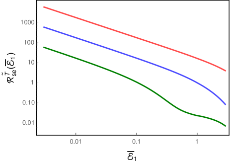
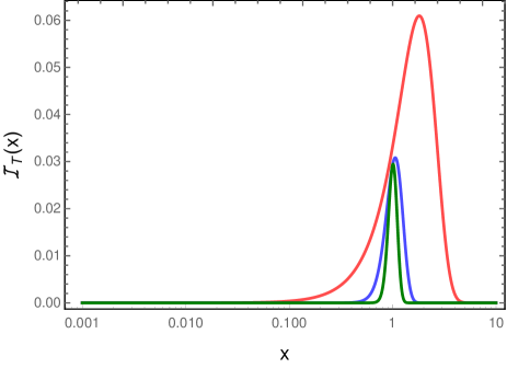
Recall that, when $\gamma_{1}\neq\gamma_{2}$ and $\Omega_{1}\to\Omega_{2}$ , $m_{0}\to\infty$ . In such a case, clearly, the condition $m_{0}\leq\hat{\mathcal{E}}$ cannot be met and the cross transition probability rate $R_{12}(\bar{\mathcal{E}}_{1})$ between the two entangled detectors will be zero. But, for the case wherein $\gamma_{1}=\gamma_{2}$ and $\Omega_{1}\neq\Omega_{2}$ , since $m_{0}=0$ , clearly, the condition $m_{0}\leq\hat{\mathcal{E}}$ is satisfied and the cross transition probability rate will be given by the above expression for $R_{12}(\bar{\mathcal{E}}_{1})$ . Evidently, in contrast to the response in the Minkowski vacuum wherein the cross transition probability rates were always zero (for the parameters we focus on), these rates can contribute non-trivially in a thermal bath for certain sets of the parameters involved. In Fig. 5, we have plotted the cross transition probability rate $R_{12}(\bar{\mathcal{E}}_{1})$ for a set of parameters that satisfy the condition $m_{0}\leq\hat{\mathcal{E}}$ and also correspond to an integer value for $m_{0}$ (in fact, for $m_{0}=0)$ .

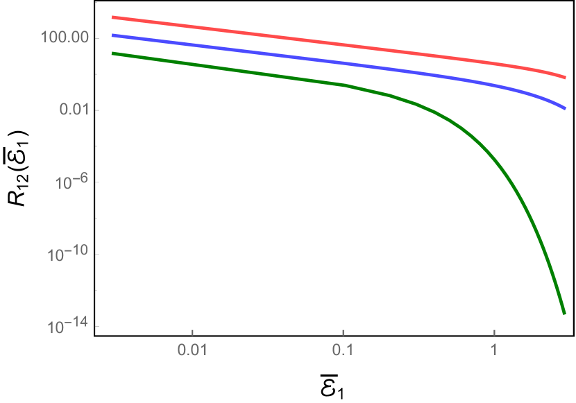
We have plotted the rate for a few different values of the dimensionless inverse temperature $\bar{\beta}_{1}$ . The figure suggests that the cross transition probability rate decreases with increasing $\bar{\beta}_{1}$ , a behavior we had encountered earlier when we had discussed the results for the case of a single detector, which corresponds to the auto transition probability rate. In the next section, we will discuss the complete transition probability of the rotating detector, including the auto and the cross transition probability rates. As we shall see, the non-zero cross transition probability rates contribute constructively and destructively for the transition from the symmetric and anti-symmetric Bell states to the collective excited state.

Lastly, it should be noted that, in the limit $\beta\to\infty$ , i.e. when the temperature of the thermal bath vanishes, the transition probability rate $R_{12}(\bar{\mathcal{E}}_{1})$ as given by Eq. (61) above reduces to zero. In the same limit, the last factor in the transition probability rate $R_{12}(\bar{\mathcal{E}}_{1})$ as given by Eq. (60) simplifies to unity and the expression reduces to the result in the Minkowski vacuum [cf. Eq. (52)], as required.

IV.2 Detectors switched on for a finite duration

Let us now turn to discuss the responses of entangled detectors that have been switched on for a finite time interval.

IV.2.1 Response in the Minkowski vacuum

As we have done earlier in the case of single detectors, let us now introduce Gaussian switching functions [cf. Eq. (30)] to examine the response of entangled detectors that are switched on for a finite time interval. In such a case, the transition probabilities (11) for two entangled detectors is given by

	$\displaystyle F_{jl}^{T}(\mathcal{E})$	$\displaystyle=$	$\displaystyle\int_{-\infty}^{\infty}{\rm d}\tau^{\prime}_{l}\int_{-\infty}^{\infty}{\rm d}\tau_{j}\,\mathrm{e}^{-i\,\mathcal{E}\,(\tau_{j}-\tau^{\prime}_{l})}\,G^{+}\left(\tau_{j},\tau^{\prime}_{l}\right)$		(62)
			$\displaystyle\times\,\exp\left[-(\tau^{2}_{j}+\tau^{\prime 2}_{l})/T^{2}\right]$		(62)

which, in terms of the variables $\bar{u}=(\tau_{j}-\tau^{\prime}_{l})$ and $\bar{v}=(\tau_{j}+\tau^{\prime}_{l})$ , can be expressed as

	$\displaystyle F_{jl}^{T}(\mathcal{E})$	$\displaystyle=$	$\displaystyle\int_{-\infty}^{\infty}\frac{{\rm d}\bar{v}}{2}\,\mathrm{e}^{-\bar{v}^{2}/(2\,T^{2})}$		(63)
			$\displaystyle\times\,\int_{-\infty}^{\infty}{\rm d}\bar{u}\,\mathrm{e}^{-i\,\mathcal{E}\,\bar{u}}\,G^{+}\left(\bar{u},\bar{v}\right)\,\mathrm{e}^{-\bar{u}^{2}/(2\,T^{2})}.\qquad$		(63)

Recall that, in the Minkowski vacuum, the Wightman function associated with the two entangled detectors that are in circular motion can be expressed as in Eq. (43). Also, as in the case of the single detector, we can define the transition probability rate of the detectors to be

R_{jl}^{T}(\mathcal{E})=\frac{F_{jl}^{T}(\mathcal{E})}{\sqrt{(\pi/2)}\,T}.

(64)

Upon substituting the Wightman function (43) in Eq. (63), we find that the corresponding transition probability rate can be expressed as

$\displaystyle R_{jl}^{T}(\mathcal{E})$	$\displaystyle=$	$\displaystyle\frac{1}{\sqrt{(\pi/2)}\,T}\int_{0}^{\infty}\frac{{\rm d}q}{4\,\pi}\sum_{m=-\infty}^{\infty}J_{m}(q\,\sigma_{j})\,J_{m}(q\,\sigma_{l})$	(65)
		$\displaystyle\times\,\int_{-\infty}^{\infty}\frac{{\rm d}\bar{v}}{2}\,\mathrm{e}^{-\left[(\bar{v}^{2}/T^{2})+i\,\alpha_{1}(q)\,\bar{v}\right]/2}$
		$\displaystyle\times\,\int_{-\infty}^{\infty}{\rm d}\bar{u}\,\mathrm{e}^{-i\,\mathcal{E}\,\bar{u}}\,\mathrm{e}^{-\left[(\bar{u}^{2}/T^{2})+i\,\alpha_{2}(q)\,\bar{u}\right]/2}.$

After carrying out the Gaussian integrals, we obtain that

	$\displaystyle R_{jl}^{T}(\mathcal{E})$	$\displaystyle=$	$\displaystyle\sqrt{2\,\pi}\,T\int_{0}^{\infty}\frac{{\rm d}q}{4\,\pi}\,\sum_{m=-\infty}^{\infty}J_{m}(q\,\sigma_{j})\,J_{m}(q\,\sigma_{l})$		(66)
			$\displaystyle\times\,\mathrm{e}^{-\left\{\alpha_{1}^{2}(q)+\left[\alpha_{2}(q)+2\,\mathcal{E}\right]^{2}\right\}\,T^{2}/8}.$		(66)

Since the integral over $q$ and the sum over $m$ do not seem to be analytically tractable, we need to compute them numerically as in the case of the single detector.

Let us first consider the auto transition probability rates of the two detectors. As we had discussed, when $j=l$ , we have $\alpha_{1}(q)=0$ and $\alpha_{2}(q)=2\,\gamma_{j}(q-m\,\Omega_{j})$ and, in such a situation, the above transition probability rate reduces to

	$\displaystyle R_{jj}^{T}(\mathcal{E})$	$\displaystyle=$	$\displaystyle\sqrt{2\,\pi}\,T\,\int_{0}^{\infty}\frac{{\rm d}q}{4\,\pi}\sum_{m=-\infty}^{\infty}\,J^{2}_{m}(q\,\sigma_{j})$		(67)
			$\displaystyle\times\,\mathrm{e}^{-\left[\mathcal{E}+\gamma_{j}\,(q-m\,\Omega_{j})\right]^{2}\,T^{2}/2}.$		(67)

Note that, as expected, this result exactly matches the transition probability rate of a single detector [cf. Eq. (35)]. We can also introduce the dimensionless variable $x_{j}=q/\Omega_{j}$ and the dimensionless parameter $\bar{T}_{j}=\gamma_{j}\,\Omega_{j}\,T$ to rewrite the above integral and sum, as we have done earlier. If we do so, we find that the result for $R_{11}^{T}(\bar{\mathcal{E}}_{1})$ is given by the expression in Eq. (37) with $(v,\gamma,\bar{\mathcal{E}},x,\bar{T})$ replaced by $(v_{1},\gamma_{1},\bar{\mathcal{E}}_{1},x_{1},\bar{T}_{1})$ . With respect to the same set of dimensionless quantities as well as the dimensionless parameters $\bar{\gamma}$ and $\bar{\Omega}$ , we find that the auto transition probability rate $R_{22}^{T}(\bar{\mathcal{E}}_{1})$ can be expressed as follows:

	$\displaystyle R_{22}^{T}(\bar{\mathcal{E}}_{1})$	$\displaystyle=$	$\displaystyle\frac{\sqrt{2\,\pi}\;\bar{T}_{1}}{4\,\pi\,\gamma_{1}}\,\int_{0}^{\infty}{\rm d}x_{1}\,\sum_{m=-\infty}^{\infty}\,J^{2}_{m}(x_{1}\,v_{2}/\bar{\Omega})$		(68)
			$\displaystyle\times\,\mathrm{e}^{-\left[\bar{\mathcal{E}}_{1}+\bar{\gamma}\,(x_{1}-\,m\,\bar{\Omega})\right]^{2}\,\bar{T}_{1}^{2}/2}.$		(68)

We should point out that, when $\bar{\gamma}=1=\bar{\Omega}$ and $v_{2}=v_{1}$ , this expression reduces to $R_{11}^{T}(\bar{\mathcal{E}}_{1})$ .

When $j=1$ and $l=2$ , we can express the cross transition probability rate $R_{12}^{T}(\bar{\mathcal{E}}_{1})$ as

$\displaystyle R_{12}^{T}(\bar{\mathcal{E}}_{1})\!\!$	$\displaystyle=$	$\displaystyle\!\!\frac{\sqrt{2\,\pi}\,\bar{T}_{1}}{4\,\pi\,\gamma_{1}}\!\sum_{m=-\infty}^{\infty}\int_{0}^{\infty}{\rm d}x_{1}\,J_{m}(x_{1}\,v_{1})\,J_{m}(x_{1}v_{2}/\bar{\Omega})$	(69)
		$\displaystyle\times\,\exp\,\biggl{(}-\biggl{\{}\left[(1-\bar{\gamma})\,x_{1}-m\,(1-\bar{\gamma}\,\bar{\Omega})\right]^{2}$
		$\displaystyle+\left[2\,\bar{\mathcal{E}}_{1}+(1+\bar{\gamma})\,x_{1}-m\,(1+\bar{\gamma}\,\bar{\Omega})\right]^{2}\biggr{\}}\,\bar{T}_{1}^{2}/8\biggr{)}$
	$\displaystyle=$	$\displaystyle R_{21}^{T}(\bar{\mathcal{E}}_{1}).$

This expression too reduces to that of $R_{11}^{T}(\mathcal{E})$ when $\bar{\gamma}=1=\bar{\Omega}$ and $v_{2}=v_{1}$ . In App. D, for convenience, we have explicitly listed the complete expressions for the finite time auto and cross transition probability rates $R_{11}^{T}(\bar{\mathcal{E}}_{1})$ , $R_{22}^{T}(\bar{\mathcal{E}}_{1})$ and $R_{12}^{T}(\bar{\mathcal{E}}_{1})$ . It is these expressions that we actually utilize to numerically compute the rates. While computing the rates, we work with the limits for the variables $x$ and $m$ for the integral and the sum that we had considered in the case of a single detector (in this context, see the caption of Fig. 3). In Fig. 6 we have plotted the above cross transition probability rate $R_{12}(\bar{\mathcal{E}}_{1})$ for a given set of parameters describing the circular motion of the detector and for different values of the dimensionless time parameter $\bar{T}_{1}$ .

We observe that the results for the cross transition probability rate are broadly similar to the auto transition probability rate we had obtained earlier in the case of a single detector (see Fig. 3). These plots also suggest that the transition probability rate is higher when the detectors interact with the field for a smaller time interval.

IV.2.2 Response in a thermal bath

We can repeat the procedure that we have adopted earlier to determine the response of two entangled detectors in circular motion and are immersed in a thermal bath. For Gaussian switching functions, we can make use of the expression (63) for the transition probability of the detectors, with the Wightman function in the thermal bath being given by Eq. (55). Upon carrying out the resulting Gaussian integrals over $\bar{u}$ and $\bar{v}$ , we find that the transition probability rate of the detectors [as defined in Eq. (64)] can be expressed as

$\displaystyle R_{jl}^{T}(\mathcal{E})$	$\displaystyle=$	$\displaystyle\sqrt{2\,\pi}\,T\int_{0}^{\infty}\frac{{\rm d}q}{4\,\pi}\,\sum_{m=-\infty}^{\infty}\,J_{m}(q\,\sigma_{j})\,J_{m}(q\,\sigma_{l})$	(70)
		$\displaystyle\times\,\biggl{\{}\frac{\mathrm{e}^{-\left\{\alpha_{1}^{2}(q)+[\alpha_{2}(q)+2\,\mathcal{E}]^{2}\right\}\,T^{2}/8}}{1-\mathrm{e}^{-\beta\,q}}$
		$\displaystyle+\,\frac{\mathrm{e}^{-\left\{\alpha_{1}^{2}(q)+[\alpha_{2}(q)-2\,\mathcal{E}]^{2}\right\}\,T^{2}/8}}{\mathrm{e}^{\beta\,q}-1}\biggr{\}}.$

When $j=l$ , since $\alpha_{1}(q)=0$ and $\alpha_{2}(q)=2\,\gamma_{j}\,(q-m\,\Omega_{j})$ , the above transition probability rate can be expressed as

$\displaystyle R_{jj}^{T}(\mathcal{E})$	$\displaystyle=$	$\displaystyle\sqrt{2\,\pi}\,T\,\int_{0}^{\infty}\frac{{\rm d}q}{4\,\pi}\,\sum_{m=-\infty}^{\infty}J^{2}_{m}(q\,\sigma_{j})$	(71)
		$\displaystyle\times\,\bigg{\{}\frac{\mathrm{e}^{-\left[\mathcal{E}+\gamma_{j}\,(q-m\,\Omega_{j})\right]^{2}\,T^{2}/2}}{1-\mathrm{e}^{-\beta\,q}}$
		$\displaystyle+\,\frac{\mathrm{e}^{-\left[\mathcal{E}-\gamma_{j}\,(q-m\,\Omega_{j})\right]^{2}\,T^{2}/2}}{\mathrm{e}^{\beta\,q}-1}\biggr{\}},$

which is essentially the transition probability rate of a single detector that we encountered earlier [cf. Eq (40)]. For instance, the transition probability rate $R_{11}^{T}(\bar{\mathcal{E}}_{1})$ is given by the expression (40) with $(v,\gamma,\bar{\mathcal{E}},\bar{\beta},\bar{T})$ replaced by $(v_{1},\gamma_{1},\bar{\mathcal{E}}_{1},\bar{\beta}_{1},\bar{T}_{1})$ . In terms of the dimensionless variables $\bar{\gamma}$ and $\bar{\Omega}$ we had introduced, we find that the transition probability rate $R_{22}^{T}(\bar{\mathcal{E}}_{1})$ can be written as

$\displaystyle R_{22}^{T}(\bar{\mathcal{E}}_{1})$	$\displaystyle=$	$\displaystyle\frac{\sqrt{2\,\pi}\;\bar{T}_{1}}{4\,\pi\,\gamma_{1}}\,\int_{0}^{\infty}{\rm d}x_{1}\,\sum_{m=-\infty}^{\infty}\,J^{2}_{m}(x_{1}\,v_{2}/\bar{\Omega})$	(72)
		$\displaystyle\times\,\biggl{\{}\frac{\mathrm{e}^{-\left[\bar{\mathcal{E}}_{1}+\bar{\gamma}\,(x_{1}-m\,\bar{\Omega})\right]^{2}\,\bar{T}_{1}^{2}/2}}{1-\mathrm{e}^{-\bar{\beta}_{1}\,x_{1}}}$
		$\displaystyle+\frac{\mathrm{e}^{-\left[\bar{\mathcal{E}}_{1}-\bar{\gamma}\,(x_{1}-m\,\bar{\Omega})\right]^{2}\,\bar{T}_{1}^{2}/2}}{\mathrm{e}^{\bar{\beta}_{1}\,x_{1}}-1}\biggr{\}}.$

Again, we can numerically compute the integral over the variable $x_{1}$ and carry out the sum over $m$ .

When $j=1$ and $l=2$ , the transition probability rate $R_{12}^{T}(\bar{\mathcal{E}}_{1})$ can be expressed as follows:

$\displaystyle R_{12}^{T}(\bar{\mathcal{E}}_{1})$	$\displaystyle=$	$\displaystyle\frac{\sqrt{2\,\pi}\,\bar{T}_{1}}{4\,\pi\,\gamma_{1}}\,\int_{0}^{\infty}{\rm d}x_{1}\sum_{m=-\infty}^{\infty}J_{m}(x_{1}\,v_{1})\,J_{m}(x_{1}\,v_{2}/\bar{\Omega})$	(73)
		$\displaystyle\times\,\biggl{(}\frac{1}{1-\mathrm{e}^{-\bar{\beta}_{1}\,x_{1}}}\,\mathrm{e}^{-\left\{\left[(1-\bar{\gamma})\,x_{1}-m\,(1-\bar{\gamma}\,\bar{\Omega})\right]^{2}+\left[(1+\bar{\gamma})\,x_{1}-m\,(1+\bar{\gamma}\,\bar{\Omega})+2\,\bar{\mathcal{E}}_{1}\right]^{2}\right\}\bar{T}_{1}^{2}/8}$
		$\displaystyle+\frac{1}{\mathrm{e}^{\bar{\beta}_{1}\,x_{1}}-1}\,\mathrm{e}^{-\left\{\left[(1-\bar{\gamma})\,x_{1}-m\,(1-\bar{\gamma}\,\bar{\Omega})\right]^{2}+\left[(1+\bar{\gamma})\,x_{1}-m\,(1+\bar{\gamma}\,\bar{\Omega})-2\,\bar{\mathcal{E}}_{1}\right]^{2}\right\}\bar{T}_{1}^{2}/8}\biggr{)}=R_{21}^{T}(\bar{\mathcal{E}}_{1}).$

This expression also reduces to $R_{11}^{T}(\mathcal{E})$ when $\bar{\gamma}=1=\bar{\Omega}$ and $v_{2}=v_{1}$ . As in the case of the response in the Minkowski vacuum, in App. D, we have provided the complete expressions for the auto and cross transition probability rates of the rotating detectors in a thermal bath. Moreover, we carry out the integral and the sum over the domain we had indicated earlier (in the caption of Fig. 3). In Fig. 7 we have plotted the cross transition probability rate $R_{12}(\bar{\mathcal{E}}_{1})$ for different values of the dimensionless time $\bar{T}_{1}$ and a fixed value of the dimensionless inverse temperature $\bar{\beta}_{1}$ .

Broadly, the cross transition probability rate exhibits the same behavior as the auto transition probability rate we had encountered earlier [cf. Fig. 3].

V Summary and discussion

In this section, we shall summarize the results we have obtained and conclude with a broader discussion.

V.1 Summary

In the previous section, we had calculated the auto and the cross transition probability rates of the two entangled detectors that are moving on circular trajectories. The auto transition probability rates of the detectors are evidently the same as the response of the single detectors we had discussed initially (in Sec. III). Note that the complete transition probability of the entangled detectors is given by the expression (9), which involves contributions from the auto and cross transition probabilities. Let us now discuss the complete probability rates for transitions from the symmetric and anti-symmetric Bell states to the excited state of the two entangled detectors.

Recall that the transition amplitude of the monopole operator is given by $m_{j}^{\omega\bar{\omega}}=\langle\bar{\omega}|\hat{m}_{j}(0)|\omega\rangle$ , with $\hat{m}_{j}(0)$ being defined in Eq. (10). As we had mentioned, for a transition from the symmetric or the anti-symmetric Bell states (i.e. from $|s\rangle$ or $|a\rangle)$ to the collective excited state (i.e. $|e\rangle)$ , the transition amplitudes of the monopole operator are found to be $m_{1}^{se}=m_{2}^{se}=1/\sqrt{2}$ and $m_{1}^{ae}=-m_{2}^{ae}=-1/\sqrt{2}$ . Due to this reason, the corresponding transition probability (9) will contain an overall factor of $1/2$ , apart from the factor of $\mu^{2}$ that arises due to the strength of the coupling between the detectors and the scalar field. Since the overall factor $\mu^{2}/2$ does not depend on either the trajectory of the detector or the state of the field, we shall drop the quantity or, equivalently, consider the total transition probability rate, say, $\mathcal{R}^{\tilde{T}}_{\omega\bar{\omega}}(\mathcal{E})$ , to be given by

\displaystyle\mathcal{R}^{\tilde{T}}_{\omega\bar{\omega}}(\mathcal{E})=\frac{2}{\mu^{2}}\,\frac{\Gamma_{|\omega\rangle\to|\bar{\omega}\rangle}(\mathcal{E})}{\tilde{T}},

(74)

where $\tilde{T}=\sqrt{(\pi/2)}\,T$ in the case of detectors that are switched on for a finite duration through the Gaussian switching functions and $\tilde{T}=\lim_{T\to\infty}T$ in the case of detectors that remain switched on forever. Therefore, the total transition probability rates from the symmetric and anti-symmetric Bell states to the collective excited state, referred to by the subscripts ‘ $se$ ’ and ‘ $ae$ ’, respectively, can be expressed as


$\displaystyle\mathcal{R}_{se}^{\tilde{T}}(\mathcal{E})\!\!$	$\displaystyle=$	$\displaystyle\!\!R_{11}^{\tilde{T}}(\mathcal{E})+R_{22}^{\tilde{T}}(\mathcal{E})+\left[R_{12}^{\tilde{T}}(\mathcal{E})+R_{21}^{\tilde{T}}(\mathcal{E})\right],$	(75a)
$\displaystyle\mathcal{R}_{ae}^{\tilde{T}}(\mathcal{E})\!\!$	$\displaystyle=$	$\displaystyle\!\!R_{11}^{\tilde{T}}(\mathcal{E})+R_{22}^{\tilde{T}}(\mathcal{E})-\left[R_{12}^{\tilde{T}}(\mathcal{E})+R_{21}^{\tilde{T}}(\mathcal{E})\right].\qquad\quad$	(75b)

Note that, in these expressions, for convenience, we have used the notation introduced above, viz. that $R_{jl}^{\tilde{T}}(\mathcal{E})$ denotes the auto or cross transition probability rate of the detectors switched on for a finite or infinite time interval.

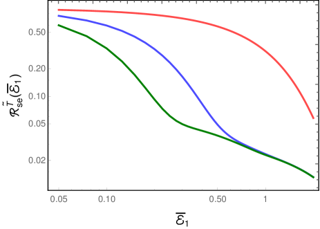
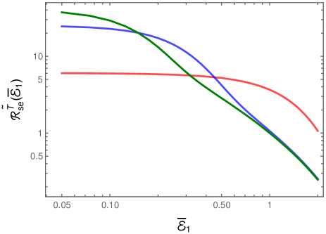
Let us first consider the case wherein the detectors are switched on for infinite duration. When the scalar field is assumed to be in the Minkowski vacuum, in the situations wherein $\gamma_{1}=\gamma_{2}$ and $\Omega_{1}\neq\Omega_{2}$ that we had focused on, the cross transition probability rates $R_{12}(\mathcal{E})$ and $R_{21}(\mathcal{E})$ vanish. This implies that the total transition probability rates $\mathcal{R}_{se}^{\tilde{T}}(\mathcal{E})$ and $\mathcal{R}_{ae}^{\tilde{T}}(\mathcal{E})$ will be equal and both the rates can be entirely expressed in terms of the auto transition probability rates $R_{11}(\mathcal{E})$ and $R_{22}(\mathcal{E})$ . As a result, the rates $\mathcal{R}_{se}^{\tilde{T}}(\mathcal{E})$ and $\mathcal{R}_{ae}^{\tilde{T}}(\bar{\mathcal{E}})$ can be expected to be similar to that of, say, $R_{11}(\mathcal{E})$ (in this regard, see Fig. 2). When the detectors are assumed to be immersed in a thermal bath of quanta associated with the scalar field, we had found that, for $\gamma_{1}=\gamma_{2}$ and $\Omega_{1}\neq\Omega_{2}$ , the cross transition probability rates $R_{12}(\mathcal{E})$ and $R_{21}(\mathcal{E})$ prove to be non-zero. Consequently, the total transition probability rates $\mathcal{R}_{se}^{\tilde{T}}(\mathcal{E})$ and $\mathcal{R}_{ae}^{\tilde{T}}(\bar{\mathcal{E}})$ can be expected to be different. This is evident from Fig. 8 where we have presented these total transition probability rates.

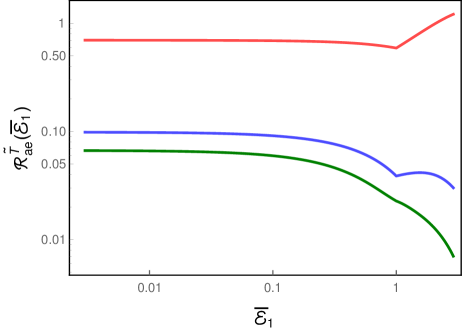
Note that the total rate $\mathcal{R}_{se}^{\tilde{T}}(\bar{\mathcal{E}}_{1})$ is about $10^{3}$ times larger in magnitude than the rate $\mathcal{R}_{se}^{\tilde{T}}(\bar{\mathcal{E}}_{1})$ for suitably small energies (in fact, for $\bar{\mathcal{E}}_{1}\lesssim 0.01)$ . These findings can provide, in principle, observable distinction in the radiative processes of entangled detectors between the Minkowski vacuum and a thermal bath.

Let us now discuss the cases wherein the detectors are switched on for a finite time interval using the Gaussian switching functions. In Fig. 9, we have plotted the total transition probability rates $\mathcal{R}_{se}^{\tilde{T}}(\mathcal{E})$ and $\mathcal{R}_{ae}^{\tilde{T}}(\bar{\mathcal{E}})$ of the entangled detectors in the Minkowski vacuum as well as the thermal bath.

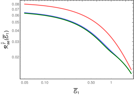
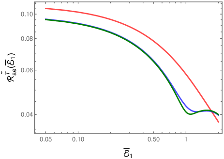
We find that the total rate $\mathcal{R}_{se}^{\tilde{T}}(\mathcal{E})$ for a transition from the symmetric Bell state to the excited state is nearly $10$ times than the total rate $\mathcal{R}_{ae}^{\tilde{T}}(\bar{\mathcal{E}})$ from the asymmetric Bell state, due to the constructive and destructive interference we mentioned above. Apart from this aspect, the total rates broadly exhibit characteristics that are similar to what we had encountered in the auto and cross transition probability rates.

V.2 Discussion

In this work, we have examined the response of detectors that are moving on circular trajectories in $(2+1)$ dimensional flat spacetime. As has been pointed out before (in this context, see, for example, Ref. Bell and Leinaas (1983)), it seems more realistic and practical to consider detectors that are in motion on circular trajectories than detectors that are moving on uniformly accelerated trajectories. We should mention that certain aspects of the response of entangled detectors that are in motion on circular trajectories have been studied earlier in the literature (see, for instance, Ref. Picanço et al. (2020)). We believe that there are many interesting aspects of the rotating detectors that we have uncovered. To begin with, we find that, in the case of two entangled, rotating detectors, the cross transition probability rates can be comparable to the auto transition probability rates of the individual detectors (cf. Figs. 5, 6, 7). Second, when the detectors are switched on for infinite duration (in both single and entangled cases), the transition probability rate of the rotating detectors in the Minkowski vacuum and a thermal bath are higher at smaller values of the energy gap of the detectors, higher values of their velocity and higher values of the temperature (cf. Fig. 2). Third, in the Minkowski vacuum, interestingly, we find that the transition probability rates of the detectors are higher when they are switched on for a shorter duration (cf. Fig. 3). Though, at first, this result may seem counter-intuitive, it can be interpreted as a manifestation of the energy-time uncertainty principle. The shorter the interval of time that the detector remains switched on, the larger can be the energy of the virtual quanta that are available to excite the detector. Fourth, in a thermal bath, when the detectors are switched on for a finite time interval, we observe that the transition probability rate is higher for smaller intervals of time only when the temperature of the thermal bath is lower or the energy gap of the detectors is higher. In fact, we observe that the behavior can be reversed at higher temperatures and smaller energy gaps (cf. Figs. 3 and 4). Fifth, from Eq. (29) and the related discussions in Sec. III, we identified a specific difference in the nature of the response of single Unruh-DeWitt detectors in a thermal bath, while they are on circular trajectories, when compared to the accelerated case. There is a single spontaneous excitation in the case of circular trajectories due to the motion, while the thermal bath contributes to the stimulated excitations. On the other hand, there are two independent, spontaneous excitations due to the motion and the thermal bath in the accelerated case, in addition to the stimulated excitation due to the thermal bath. Finally, as we had discussed in the previous subsection, due to constructive or destructive interference, the total transition probability rates from the symmetric and anti-symmetric Bell states to the collective excited state can be substantially different in a thermal bath or when they are switched on for a finite time interval in the Minkowski vacuum. We should mention that a similar behavior is also observed when one considers the de-excitation of the detector from the symmetric or the anti-symmetric Bell states to the ground state (in this regard, see the discussion in Refs. Ficek and Tanaś (2002); Menezes and Svaiter (2015)).

There are many further aspects of the rotating and entangled detectors that remain to be explored. We need to urgently extend all our analysis to $(3+1)$ -spacetime dimensions. In $(3+1)$ -spacetime dimensions, while we expect the results to be qualitatively similar to the $(2+1)$ -dimensional case we have considered here, we can expect some quantitative differences. Also, we have to examine whether two initially uncorrelated atomic detectors moving on circular trajectories can get entangled over time, a phenomenon that has been referred to as entanglement harvesting (in this regard, see Refs. Reznik (2003); Martin-Martinez et al. (2016); Koga et al. (2018, 2019); Barman et al. (2021a, b)). In particular, we need to investigate entanglement harvesting in the presence of a thermal bath, with detectors switched on for infinite as well as finite intervals of time (for previous studies in this context involving static and non-inertial detectors in a thermal bath, see Refs. Brown (2013); Simidzija and Martín-Martínez (2018) and Ref. Barman et al. (2021a), respectively). Moreover, it will be interesting to study the effects due to the presence of boundaries Davies et al. (1996); Picanço et al. (2020). Further, on the practical front, it is easier to set charged particles in motion on circular trajectories, using, say, with the help of an external magnetic field. If a charged particle (say, an ion) is to be used as a detector, then it may emit classical synchrotron radiation as it moves along the circular trajectories. We need to understand the implications or effects of the synchrotron radiation for the detection of quanta emitted or absorbed by the detector due to the quantum phenomena we are investigating. We are presently working on these issues.

Acknowledgements.

SB would like to thank the Science and Engineering Research Board, Government of India, for supporting this work through the National Postdoctoral Fellowship PDF/2022/000428.

Appendix A Wightman function in polar coordinates

In $(2+1)$ -dimensional flat spacetime, when working in the Cartesian coordinates ${\bm{x}}=(x,y)$ , the Wightman function associated with a massive, minimally coupled, scalar field can be written as (in this regard, see, for instance, Ref. Birrell and Davies (1984b))

\displaystyle G^{+}(\tilde{x},\tilde{x}^{\prime})=\int\frac{{\rm d}^{2}{\bm{k}}}{(2\,\pi)^{2}\,(2\,\omega)}\,\mathrm{e}^{-i\,\omega\,(t-t^{\prime})+i\,{\bm{k}}\cdot({\bm{x}}-{\bm{x}}^{\prime})},

(76)

where $\omega=(|{\bm{k}}|^{2}+\mu^{2})^{1/2}$ , and $\mu$ denotes the mass of the field. Let us write both the wave vector ${\bm{k}}$ and the position vector ${\bm{x}}$ in terms of the corresponding polar coordinates, say, $(q,\alpha)$ and $(\rho,\phi)$ , as follows:


$\displaystyle k_{x}$	$\displaystyle=$	$\displaystyle q\,\cos{\alpha},\quad\;k_{y}=q\,\sin{\alpha},$	(77a)
$\displaystyle x$	$\displaystyle=$	$\displaystyle\rho\,\cos{\phi},\quad\;\;\,y=\rho\,\sin{\phi},$	(77b)
$\displaystyle x^{\prime}$	$\displaystyle=$	$\displaystyle\rho^{\prime}\,\cos{\phi^{\prime}},\quad y^{\prime}=\rho^{\prime}\,\sin{\phi^{\prime}}.$	(77c)

In such a case, the Wightman function (76) can be expressed as

	$\displaystyle G^{+}(\tilde{x},\tilde{x}^{\prime})$	$\displaystyle=$	$\displaystyle\int_{0}^{\infty}\frac{{\rm d}q\,q}{(2\,\pi)\,(2\,\omega)}\int_{0}^{2\,\pi}\frac{{\rm d}\alpha}{2\,\pi}\,\mathrm{e}^{-i\,\omega\,(t-t^{\prime})}$		(78)
			$\displaystyle\times\,\mathrm{e}^{i\,q\,\left[\rho\,\cos(\phi-\alpha)-\rho^{\prime}\,\cos(\phi^{\prime}-\alpha)\right]}.$		(78)

If we now use the following identity (known as the Jacobi–Anger identity; in this context, see, for instance, Ref. Arfken (1985))

\displaystyle\mathrm{e}^{i\,z\,\cos{\phi}}=\sum_{m=-\infty}^{\infty}i^{m}\,J_{m}(z)\,\mathrm{e}^{i\,m\,\phi},

(79)

where $J_{m}(z)$ are the Bessel functions, then the Wightman function can be written as

$\displaystyle G^{+}(\tilde{x},\tilde{x}^{\prime})$	$\displaystyle=$	$\displaystyle\int_{0}^{\infty}\frac{{\rm d}q\,q}{(2\,\pi)\,(2\,\omega)}\,\int_{0}^{2\pi}\,\frac{{\rm d}\alpha}{2\,\pi}\,\mathrm{e}^{-i\,\omega\,(t-t^{\prime})}$
		$\displaystyle\times\,\sum_{m=-\infty}^{\infty}i^{m}\,J_{m}(q\,\rho)\,\mathrm{e}^{i\,m\,(\phi-\alpha)}\,$
		$\displaystyle\times\,\sum_{m^{\prime}=-\infty}^{\infty}i^{m^{\prime}}\,J_{m^{\prime}}(-q\,\rho^{\prime})\,\mathrm{e}^{i\,m^{\prime}\,(\phi^{\prime}-\alpha)}$
	$\displaystyle=$	$\displaystyle\int_{0}^{\infty}\frac{{\rm d}q\,q}{4\,\pi\,\omega}\,\mathrm{e}^{-i\,\omega\,(t-t^{\prime})}$
		$\displaystyle\times\,\sum_{m=-\infty}^{\infty}J_{m}(q\,\rho)\,J_{-m}(-q\,\rho^{\prime})\,\mathrm{e}^{i\,m\,(\phi-\phi^{\prime})}.$

We should mention that, to arrive at the final equality, we have used the relation

\int_{0}^{2\,\pi}{\rm d}\alpha\,\mathrm{e}^{-i\,(m+m^{\prime})\,\alpha}=(2\,\pi)\,\delta_{m,-m^{\prime}},

(81)

where $\delta_{n,n^{\prime}}$ denotes the Kronecker delta. On using the identity $J_{-m}(-q\,\rho^{\prime})=J_{m}(q\,\rho^{\prime})$ , in the case of a massless field (i.e. when $\mu=0$ so that $\omega=q$ ), we can arrive at the expression (19) for the Wightman function we have mentioned earlier.

Similarly, when working in the Cartesian coordinates, the Wightman function for the scalar field at a finite temperature in $(2+1)$ spacetime dimensions can be easily obtained to be (see, for instance, Ref. Birrell and Davies (1984b); Kolekar and Padmanabhan (2014); Chowdhury et al. (2019))

	$\displaystyle G_{\beta}^{+}(\tilde{x},\tilde{x}^{\prime})$	$\displaystyle=$	$\displaystyle\int\frac{{\rm d}^{2}{\bm{k}}}{(2\,\pi)^{2}\,(2\,\omega)}\,\biggl{\{}\frac{\mathrm{e}^{-i\,\left[\omega\,(t-t^{\prime})-{\bm{k}}\cdot({\bm{x}}-{\bm{x}}^{\prime})\right]}}{1-\mathrm{e}^{-\beta\,\omega}}$		(82)
			$\displaystyle+\frac{\mathrm{e}^{i\,\left[\omega\,(t-t^{\prime})-{\bm{k}}\cdot({\bm{x}}-{\bm{x}}^{\prime})\right]}}{\mathrm{e}^{\beta\,\omega-1}}\biggr{\}}.$		(82)

In the case of a massless field, upon carrying out the transformations (77), we can arrive at the expression for the above Wightman function in terms of the polar coordinates (in both real and momentum space), which is the result (24) we have quoted earlier.

Appendix B Behavior of the transition probability rate as a function of velocity of the detector

In our discussion, barring in Fig. 4, we have been primarily interested in computing the auto and cross transition probability rates of the detectors as a function of the energy gap $\mathcal{E}$ , for given angular and linear velocities $\Omega$ and $v$ of the detector, inverse temperature $\beta$ of the thermal bath and the time interval $T$ for which the detector is switched on. We had pointed out that the sums over $m$ which appear in the transition probability rates converge fairly quickly. Specifically, we had mentioned that, for the parameters we have considered, it is adequate to evaluate the sum until $(m-\bar{\mathcal{E}})=50$ and $(m-\bar{\mathcal{E}})=10$ when the detectors are switched on for infinite or a finite duration (in this regard, see the captions of Figs. 2 and 3). However, when the detector is switched on for infinite duration, as we had discussed in Sec. III [see our discussion following Eq. (23)], the convergence of the sum depends on the velocity of the detector. We find that, for detector velocities very close to the velocity of light (say, for $v\gtrsim 0.9$ ), it becomes necessary to evaluate the sum to larger values of $m$ . To illustrate this point, in Fig. 10, we have plotted the transition probability rate of the rotating detector in the Minkowski vacuum as a function of the linear velocity $v$ of the detector.

We have fixed the value of the energy gap $\mathcal{E}$ in plotting the results and have assumed that the detector remains switched on forever. Note that, for $v\gtrsim 0.9$ , the peak in the transition probability rate of the detector shifts towards higher velocities as we sum to larger and larger values of $m$ . In the results we have presented in all the earlier figures, we have ensured that, for the parameters we have worked with, summing to larger values of $m$ does not significantly change the results we obtain.

Appendix C Behavior of the integrand in the finite time transition probability rate

Recall that, in the case of detectors that are switched on for a finite time interval, we have to carry out an integral over $x$ , apart from summing over $m$ . Immediately after Eq. (37), we had discussed the behavior of the integrals at large and small values of $x$ . In this appendix, we shall briefly illustrate the behavior of the integrands that are encountered when evaluating the response of the detector in the Minkowski vacuum. Note that the integrands in this case are of the following form:

	$\displaystyle\mathcal{I}_{T}(x)$	$\displaystyle=$	$\displaystyle J^{2}_{m}(x\,v)\,\mathrm{e}^{-\left[(x^{2}/2)+x\,\bar{\mathcal{E}}\right]\,\bar{T}^{2}}\,\mathrm{e}^{-m^{2}\,\bar{T}^{2}/2}$		(83)
			$\displaystyle\times\,\mathrm{cosh}\left[m\,(x+\bar{\mathcal{E}})\,\bar{T}^{2}\right].$		(83)

In Fig. 11, we have plotted this integrand for $m=0$ and $m=1$ and a few different values of the dimensionless time interval $\bar{T}$ , assuming fixed values for the velocity $v$ and the dimensionless energy gap $\bar{\mathcal{E}}$ .

It is evident that the integrands are well behaved and, in particular, they decrease rapidly at large $x$ due to the $\mathrm{e}^{-x^{2}\,\bar{T}^{2}/2}$ factor. Moreover, for $m>0$ , the factor $\mathrm{e}^{-m^{2}\,\bar{T}^{2}/2}$ also suppresses the overall amplitude of the integrand. Such a rapid decrease allows us to quickly compute the integrals involved. As we had mentioned, for the values of the parameters we work with, we find that it is adequate to integrate up to $x=10^{2}$ (see the caption of Fig. 3) and we have also checked that the results we obtain are not altered if we increase the upper limit.

Appendix D Transition probability rates of entangled detectors for finite duration

In this appendix, we shall provide explicit expressions for the transition probability rates of the entangled detectors that are moving on circular trajectories and are interacting with the scalar field for a finite time interval. It is these expressions that we eventually use to numerically compute the transition probability rates.

Let us first consider the case of the Minkowski vacuum. We find that the expressions (67) and (68) can be utilized to write $R_{11}^{T}(\bar{\mathcal{E}}_{1})$ and $R_{22}^{T}(\bar{\mathcal{E}}_{1})$ as


$\displaystyle R_{11}^{T}(\bar{\mathcal{E}}_{1})$	$\displaystyle=$	$\displaystyle\frac{\sqrt{2\,\pi}\;\bar{T}_{1}}{4\,\pi\,\gamma_{1}}\,\mathrm{e}^{-\bar{\mathcal{E}}_{1}^{2}\,\bar{T}_{1}^{2}/2}\,\Biggl{\{}\int_{0}^{\infty}{\rm d}x_{1}\,J^{2}_{0}(x_{1}\,v_{1})\,\mathrm{e}^{-\left[(x_{1}^{2}/2)+x_{1}\,\bar{\mathcal{E}}_{1}\right]\,\bar{T}_{1}^{2}}$	(84a)
		$\displaystyle+\,2\,\sum_{m=1}^{\infty}\,\mathrm{e}^{-m^{2}\,\bar{T}_{1}^{2}/2}\int_{0}^{\infty}{\rm d}x_{1}\,J^{2}_{m}(x_{1}\,v_{1})\,\mathrm{e}^{-\left[(x_{1}^{2}/2)+x_{1}\,\bar{\mathcal{E}}_{1}\right]\,\bar{T}_{1}^{2}}\,\mathrm{cosh}\left[m\,(x_{1}+\bar{\mathcal{E}}_{1})\,\bar{T}_{1}^{2}\right]\Biggr{\}}\,,$	(84a)
$\displaystyle R_{22}^{T}(\mathcal{E})$	$\displaystyle=$	$\displaystyle\frac{\sqrt{2\,\pi}\;\bar{T}_{1}}{4\,\pi\,\gamma_{1}}\,\mathrm{e}^{-\bar{\mathcal{E}}_{1}^{2}\,\bar{T}_{1}^{2}/2}\,\Biggl{\{}\int_{0}^{\infty}{\rm d}x_{1}\,J^{2}_{0}\left(x_{1}\,v_{2}/\bar{\Omega}\right)\,\mathrm{e}^{-\left[(x_{1}^{2}/2)+x_{1}\,\bar{\mathcal{E}}_{1}/\bar{\gamma}\right]\,\bar{\gamma}^{2}\,\bar{T}_{1}^{2}}$	(84b)
		$\displaystyle+\,2\,\sum_{m=1}^{\infty}\,\mathrm{e}^{-m^{2}\,\bar{\gamma}^{2}\,\bar{\Omega}^{2}\,\bar{T}_{1}^{2}/2}\,\int_{0}^{\infty}{\rm d}x_{1}\,J^{2}_{m}\left(x_{1}v_{2}/\bar{\Omega}\right)\,\mathrm{e}^{-\left[(x_{1}^{2}/2)+x_{1}\,\bar{\mathcal{E}}_{1}/\bar{\gamma}\right]\,\bar{\gamma}^{2}\,\bar{T}_{1}^{2}}$
		$\displaystyle\times\,\mathrm{cosh}\left[m\,\left(x_{1}+\bar{\mathcal{E}}_{1}/\bar{\gamma}\right)\,\bar{\gamma}^{2}\,\bar{\Omega}\,\bar{T}_{1}^{2}\right]\Biggr{\}}.\qquad\quad$

Similarly, the expression (69) for the cross transition probability rate $R_{12}^{T}(\bar{\mathcal{E}}_{1})$ in the Minkowski vacuum can be written as

$\displaystyle R_{12}^{T}(\bar{\mathcal{E}}_{1})$	$\displaystyle=$	$\displaystyle\frac{\sqrt{2\,\pi}\,\bar{T}_{1}}{4\,\pi\,\gamma_{1}}\,\mathrm{e}^{-\bar{\mathcal{E}}_{1}^{2}\,\bar{T}_{1}^{2}/2}\,\Biggl{(}\int_{0}^{\infty}{\rm d}x_{1}\,J_{0}(x_{1}\,v_{1})\,J_{0}(x_{1}\,v_{2}/\bar{\Omega})\,\mathrm{e}^{-\left[(1+\bar{\gamma}^{2})\,x_{1}^{2}+2\,(1+\bar{\gamma})\,x_{1}\,\bar{\mathcal{E}}_{1}\right]\,\bar{T}_{1}^{2}/4}$	(85)
		$\displaystyle+\,2\,\sum_{m=1}^{\infty}\,\mathrm{e}^{-m^{2}\,(1+\bar{\gamma}^{2}\,\bar{\Omega}^{2})\,\bar{T}_{1}^{2}/4}\int_{0}^{\infty}{\rm d}x_{1}\,J_{m}(x_{1}\,v_{1})\,J_{m}(x_{1}\,v_{2}/\bar{\Omega})\,\mathrm{e}^{-\left[(1+\bar{\gamma}^{2})\,x_{1}^{2}+2\,(1+\bar{\gamma})\,x_{1}\,\bar{\mathcal{E}}_{1}\right]\,\bar{T}_{1}^{2}/4}$
		$\displaystyle\times\,\mathrm{cosh}\left\{m\,\left[(1+\bar{\gamma}^{2}\,\bar{\Omega})\,x_{1}+(1+\bar{\gamma}\,\bar{\Omega})\,\bar{\mathcal{E}}_{1}\right]\,\bar{T}_{1}^{2}/2\right\}\Biggr{)}=R_{21}^{T}(\bar{\mathcal{E}}_{1}).$

The expressions (71) and (72) can be used to write the auto transition probability rates of the rotating detectors in a thermal bath as


$\displaystyle R_{11}^{T}(\bar{\mathcal{E}}_{1})$	$\displaystyle=$	$\displaystyle\frac{\sqrt{2\,\pi}\;\bar{T}_{1}}{4\,\pi\,\gamma_{1}}\,\mathrm{e}^{-\bar{\mathcal{E}}_{1}^{2}\,\bar{T}_{1}^{2}/2}\,\Biggl{\{}\int_{0}^{\infty}{\rm d}x_{1}\,J^{2}_{0}(x_{1}\,v_{1})\,\left[\frac{\mathrm{e}^{-\left[(x_{1}^{2}/2)+x_{1}\,\bar{\mathcal{E}}_{1}\right]\,\bar{T}_{1}^{2}}}{1-\mathrm{e}^{-\bar{\beta}_{1}\,x_{1}}}+\frac{\mathrm{e}^{-\left[(x_{1}^{2}/2)-x_{1}\,\bar{\mathcal{E}}_{1}\right]\,\bar{T}_{1}^{2}}}{\mathrm{e}^{\bar{\beta}_{1}\,x_{1}}-1}\,\right]$	(86a)
		$\displaystyle+\,2\,\sum_{m=1}^{\infty}\,\mathrm{e}^{-m^{2}\,\bar{T}_{1}^{2}/2}\int_{0}^{\infty}{\rm d}x_{1}\,J^{2}_{m}(x_{1}\,v_{1})\,\biggl{[}\frac{\mathrm{e}^{-\left[(x_{1}^{2}/2)+x_{1}\,\bar{\mathcal{E}}_{1}\right]\,\bar{T}_{1}^{2}}}{1-\mathrm{e}^{-\bar{\beta}_{1}\,x_{1}}}\,\mathrm{cosh}\left[m\,(x_{1}+\bar{\mathcal{E}}_{1})\,\bar{T}_{1}^{2}\right]$
		$\displaystyle+\,\frac{\mathrm{e}^{-\left[(x_{1}^{2}/2)-x_{1}\,\bar{\mathcal{E}}_{1}\right]\,\bar{T}_{1}^{2}}}{\mathrm{e}^{\bar{\beta}_{1}\,x_{1}}-1}\,\mathrm{cosh}\left[m\,(x_{1}-\bar{\mathcal{E}}_{1})\,\bar{T}_{1}^{2}\right]\Biggr{\}},$
$\displaystyle R_{22}^{T}(\bar{\mathcal{E}}_{1})$	$\displaystyle=$	$\displaystyle\frac{\sqrt{2\,\pi}\;\bar{T}_{1}}{4\,\pi\gamma_{1}}\,\mathrm{e}^{-\bar{\mathcal{E}}_{1}^{2}\,\bar{T}_{1}^{2}/2}\,\Biggl{(}\int_{0}^{\infty}{\rm d}x_{1}\,J^{2}_{0}\left(\frac{x_{1}\,v_{2}}{\bar{\Omega}}\right)\,\left[\frac{\mathrm{e}^{-\left[(x_{1}^{2}/2)+x_{1}\,\bar{\mathcal{E}}_{1}/\bar{\gamma}\right]\,\bar{\gamma}^{2}\,\bar{T}_{1}^{2}}}{1-\mathrm{e}^{-\bar{\beta}_{1}\,x_{1}}}+\frac{\mathrm{e}^{-\left[(x_{1}^{2}/2)-x_{1}\,\bar{\mathcal{E}}_{1}/\bar{\gamma}\right]\,\bar{\gamma}^{2}\,\bar{T}_{1}^{2}}}{\mathrm{e}^{\bar{\beta}_{1}\,x_{1}}-1}\right]$	(86b)
		$\displaystyle+\,2\,\sum_{m=1}^{\infty}\,\mathrm{e}^{-m^{2}\,\bar{\gamma}^{2}\,\bar{\Omega}^{2}\,\bar{T}_{1}^{2}/2}\,\int_{0}^{\infty}{\rm d}x_{1}\,J^{2}_{m}\left(x_{1}v_{2}/\bar{\Omega}\right)\,\biggl{\{}\frac{\mathrm{e}^{-\left[(x_{1}^{2}/2)+x_{1}\,\bar{\mathcal{E}}_{1}/\bar{\gamma}\right]\,\bar{\gamma}^{2}\,\bar{T}_{1}^{2}}}{1-\mathrm{e}^{-\bar{\beta}_{1}\,x_{1}}}\,\mathrm{cosh}\left[m\,\left(x_{1}+\frac{\bar{\mathcal{E}}_{1}}{\bar{\gamma}}\right)\,\bar{\gamma}^{2}\,\bar{\Omega}\,\bar{T}_{1}^{2}\right]$
		$\displaystyle+\,\frac{\mathrm{e}^{-\left[(x_{1}^{2}/2)-x_{1}\,\bar{\mathcal{E}}_{1}/\bar{\gamma}\right]\,\bar{\gamma}^{2}\,\bar{T}_{1}^{2}}}{\mathrm{e}^{\bar{\beta}_{1}\,x_{1}}-1}\mathrm{cosh}\left[m\left(x_{1}-\frac{\bar{\mathcal{E}}_{1}}{\bar{\gamma}}\right)\,\bar{\gamma}^{2}\,\bar{\Omega}\,\bar{T}_{1}^{2}\right]\biggr{\}}\Biggr{)}.$

Similarly, upon using the expression (73), the corresponding cross transition transition probability rate $R_{12}^{T}(\bar{\mathcal{E}}_{1})$ can be written as

$\displaystyle R_{12}^{T}(\bar{\mathcal{E}}_{1})$	$\displaystyle=$	$\displaystyle\frac{\sqrt{2\,\pi}\;\bar{T}_{1}}{4\,\pi\,\gamma_{1}}\,\mathrm{e}^{-\bar{\mathcal{E}}_{1}^{2}\,\bar{T}_{1}^{2}/2}\,\Biggl{[}\int_{0}^{\infty}{\rm d}x_{1}\,J_{0}(x_{1}\,v_{1})\,J_{0}(x_{1}\,v_{2}/\bar{\Omega})\,\biggl{[}\frac{\mathrm{e}^{-\left[(1+\bar{\gamma}^{2})\,x_{1}^{2}+2\,(1+\bar{\gamma})\,x_{1}\,\bar{\mathcal{E}}_{1}\right]\,\bar{T}_{1}^{2}/4}}{1-\mathrm{e}^{-\bar{\beta}_{1}\,x_{1}}}\,$	(87)
		$\displaystyle+\,\frac{\mathrm{e}^{-\left[(1+\bar{\gamma}^{2})\,x_{1}^{2}-2\,(1+\bar{\gamma})\,x_{1}\,\bar{\mathcal{E}}_{1}\right]\,\bar{T}_{1}^{2}/4}}{\mathrm{e}^{\bar{\beta}_{1}\,x_{1}}-1}\biggr{]}$
		$\displaystyle+\,2\,\sum_{m=1}^{\infty}\,\mathrm{e}^{-m^{2}\,(1+\bar{\gamma}^{2}\,\bar{\Omega}^{2})\,\bar{T}_{1}^{2}/4}\,\int_{0}^{\infty}{\rm d}x_{1}\,J_{m}(x_{1}\,v_{1})\,J_{m}(x_{1}\,v_{2}/\bar{\Omega})$
		$\displaystyle\times\,\bigg{(}\frac{\mathrm{e}^{-\left[(1+\bar{\gamma}^{2})\,x_{1}^{2}+2\,(1+\bar{\gamma})\,x_{1}\,\bar{\mathcal{E}}_{1}\right]\,\bar{T}_{1}^{2}/4}}{1-\mathrm{e}^{-\bar{\beta}_{1}\,x_{1}}}\,\mathrm{cosh}\left\{m\,\left[(1+\bar{\gamma}^{2}\,\bar{\Omega})\,x_{1}+(1+\bar{\gamma}\,\bar{\Omega})\,\bar{\mathcal{E}}_{1}\right]\,\bar{T}_{1}^{2}/2\right\}$
		$\displaystyle+\,\frac{\mathrm{e}^{-\left[(1+\bar{\gamma}^{2})\,x_{1}^{2}-2\,(1+\bar{\gamma})\,x_{1}\,\bar{\mathcal{E}}_{1}\right]\,\bar{T}_{1}^{2}/4}}{\mathrm{e}^{\bar{\beta}_{1}\,x_{1}}-1}\,\mathrm{cosh}\left\{m\,\left[(1+\bar{\gamma}^{2}\,\bar{\Omega})\,x_{1}-(1+\bar{\gamma}\,\bar{\Omega})\,\bar{\mathcal{E}}_{1}\right]\,\bar{T}_{1}^{2}/2\right\}\biggr{)}\Biggr{]}=R_{21}^{T}(\bar{\mathcal{E}}_{1}).$

Appendix E A remedy for the infrared divergence

In our analysis, we had encountered an infrared divergence when calculating the Wightman function at a finite temperature. The occurrence of infrared divergences in Green’s functions in spacetime dimensions less than $(3+1)$ is not uncommon. We can turn to the calculation of the Green’s functions in $(1+1)$ -spacetime dimensions to identify possible remedies to regulate the divergence (in this context, see, for example, Ref. Chowdhury et al. (2019)). Note that, in the case of $(2+1)$ -spacetime dimensions, we encounter the divergence only when calculating the Green’s function at a finite temperature. (We should clarify that such a divergence does not arise in $(3+1)$ -spacetime dimensions.) Also, the divergence occurs only in the $m=0$ term in the sum in Eq. (25). In the case wherein the detectors are switched on forever, the divergence in the Wightman function does not affect the transition probability rate of the detector, as the $m=0$ term does not contribute [cf. Eq. (26)]. We should mention here that such a behavior has also been noticed earlier in a related work Barman et al. (2021b). However, when we consider detectors that are switched on for a finite duration, the $m=0$ term in Eq. (40) leads to a non-zero contribution and we need to formally regulate the divergence. We need to do so in such a way that we recover the result in the limit of $\bar{\beta}\to\infty$ [viz. Eq. (37)], i.e. when the temperature of the thermal bath vanishes. Needless to add, we also need to reproduce our earlier result (26) at a finite temperature for the case of detectors that remain switched on forever (i.e in the limit $\bar{T}\to\infty$ ).

Let us first single out the term containing the infrared divergence in the finite temperature Wightman function (25). Using the following identity (cf. Ref. Gradshteyn and Ryzhik (2007), 8.531.1):

J_{0}^{2}(z)+2\sum_{m=1}^{\infty}\,J_{m}^{2}(z)=1,

(88)

we can express the Wightman function (25) as

\displaystyle G^{+}_{\beta}(u)=\mathcal{A}_{0}(u)+\mathcal{A}_{1}(u),

(89)

where the quantities $\mathcal{A}_{0}(u)$ and $\mathcal{A}_{1}(u)$ are given by


$\displaystyle\mathcal{A}_{0}(u)$	$\displaystyle=$	$\displaystyle\int_{0}^{\infty}\frac{{\rm d}q}{4\,\pi}\,\left(\frac{\mathrm{e}^{-i\,\gamma\,q\,u}}{1-\mathrm{e}^{-\beta\,q}}+\frac{\mathrm{e}^{i\,\gamma\,q\,u}}{\mathrm{e}^{\beta\,q}-1}\right),$	(90a)
$\displaystyle\mathcal{A}_{1}(u)$	$\displaystyle=$	$\displaystyle\int_{0}^{\infty}\frac{{\rm d}q}{4\,\pi}\,\biggl{\{}\sum_{\begin{subarray}{c}m=-\infty\\ m\neq 0\end{subarray}}^{\infty}J^{2}_{m}(q\,\sigma)$	(90b)
		$\displaystyle\times\,\left[\frac{\mathrm{e}^{-i\,\gamma\,(q-m\,\Omega)\,u}}{1-\mathrm{e}^{-\beta\,q}}+\frac{\mathrm{e}^{i\,\gamma\,(q-m\,\Omega)\,u}}{\mathrm{e}^{\beta\,q}-1}\right]~{}$
		$\displaystyle-\,2\,\left(\frac{\mathrm{e}^{-i\,\gamma\,q\,u}}{1-\mathrm{e}^{-\beta\,q}}+\frac{\mathrm{e}^{i\,\gamma\,q\,u}}{\mathrm{e}^{\beta\,q}-1}\right)$
		$\displaystyle\times\,\sum_{m=1}^{\infty}J^{2}_{m}(q\,\sigma)\biggr{\}}.$

Therefore, the transition probability rate of a detector switched on for a finite time through the Gaussian window function can be expressed as

\displaystyle R_{T}(\mathcal{E})

\displaystyle=

\displaystyle R_{T}^{0}(\mathcal{E})+R_{T}^{1}(\mathcal{E})~{},

(91)

where, evidently, $R_{T}^{0,1}(\mathcal{E})$ are given by

R_{T}^{0,1}(\mathcal{E})=\int_{-\infty}^{\infty}{\rm d}u\,\mathrm{e}^{-i\,\mathcal{E}\,u}\,\mathcal{A}_{0,1}(u)\,\mathrm{e}^{-u^{2}/(2\,T^{2})}.

(92)

Since the term $\mathcal{A}_{1}(u)$ in the finite temperature Wightman function does not contain the infrared divergence, the corresponding transition probability rate $R_{T}^{1}(\mathcal{E})$ can be evaluated as we have done earlier in the other cases. Therefore, let us turn to the calculation of the rate $R_{T}^{0}(\mathcal{E})$ that depends on the term $\mathcal{A}_{0}(u)$ . To do so, let us first explicitly evaluate $\mathcal{A}_{0}(u)$ . As is often done in the case of $(1+1)$ -spacetime dimensions, in order to avoid the divergence, we shall take the derivative of $\mathcal{A}_{0}(u)$ with respect to the variable $u$ , thus rendering it safe from the infrared divergence. We can then evaluate the integral over $q$ as usual, by introducing an ultraviolet regulator of the form of $\mathrm{e}^{-\epsilon\,q}$ to obtain that

	$\displaystyle\frac{\partial\mathcal{A}_{0}(u)}{\partial u}$	$\displaystyle=$	$\displaystyle-\frac{i\,\gamma}{4\,\pi\,\beta^{2}}\,\biggl{[}\psi^{(1)}\left(\frac{i\,\gamma\,u+\epsilon}{\beta}\right)$		(93)
			$\displaystyle-\,\psi^{(1)}\left(\frac{-i\,\gamma\,u+\beta+\epsilon}{\beta}\right)\biggr{]},$		(93)

where $\psi^{(n)}(z)$ denotes the polygamma function of order $n$ . Upon integrating over $u$ , we arrive at the expression

	$\displaystyle\mathcal{A}_{0}(u)$	$\displaystyle=$	$\displaystyle-\frac{1}{4\pi\beta}\,\biggl{[}\psi^{(0)}\left(\frac{i\,\gamma\,u+\epsilon}{\beta}\right)$		(94)
			$\displaystyle+\,\psi^{(0)}\left(\frac{-i\,\gamma\,u+\beta+\epsilon}{\beta}\right)\biggr{]}.$		(94)

In the limit of zero temperature (i.e. as $\beta\to\infty$ ), this expression reduces to

\displaystyle\lim_{\beta\to\infty}\mathcal{A}_{0}(u)

\displaystyle=

\displaystyle-\frac{i}{4\,\pi}\,\frac{1}{\gamma\,u-i\,\epsilon}

(95)

which is the result we would have obtained had we taken the limit $\beta\to\infty$ in Eq. (90a) (i.e. before taking the derivative and carrying out the integration with respect to variable $u$ ).

We can now evaluate the transition probability rate $R_{T}^{0}(\mathcal{E})$ of the detector using the expression (94) for $\mathcal{A}_{0}(u)$ . To do so, let us define the dimensionless variable $\tilde{u}=\gamma\,\Omega\,u$ and parameter $\bar{\epsilon}=\epsilon\,\Omega$ . Let us also make use of the Fourier transform

\mathrm{e}^{-\tilde{u}^{2}/(2\,\bar{T}^{2})}=\frac{\bar{T}}{\sqrt{2\,\pi}}\,\int_{-\infty}^{\infty}{\rm d}\xi\,\mathrm{e}^{i\,\tilde{u}\,\xi-\xi^{2}\,\bar{T}^{2}/2}

(96)

and the following series expansion of the polygamma function:

\psi^{(0)}(z)=-\sum_{k=0}^{\infty}\frac{1}{(z+k)}.

(97)

From this last expression, it would be clear that the first and the second polygamma functions in Eq. (94) would have poles at $\tilde{u}=i\,(k\,\bar{\beta}+\bar{\epsilon})=i\,p_{1}(k)$ (i.e. in the upper half of the complex $\tilde{u}$ -plane) and at $\tilde{u}=-i\,[(k+1)\,\bar{\beta}+\bar{\epsilon}]=-i\,p_{2}(k)$ (i.e. in the lower half of the complex $\tilde{u}$ -plane), respectively. The transition probability rate $R_{T}^{0}(\mathcal{E})$ can be written as

\displaystyle R_{T}^{0}(\mathcal{E})

\displaystyle=

\displaystyle\frac{\bar{T}}{4\,\pi\,i\,\,\gamma\,\sqrt{2\,\pi}}\,\sum_{k=0}^{\infty}\int_{-\infty}^{\infty}{\rm d}\xi\,\mathrm{e}^{-\xi^{2}\,\bar{T}^{2}/2}\int_{-\infty}^{\infty}{\rm d}\tilde{u}\,\mathrm{e}^{i\,(\xi-\bar{\mathcal{E}})\,\tilde{u}}\,\left[\frac{1}{\tilde{u}-i\,p_{1}(k)}-\frac{1}{\tilde{u}+i\,p_{2}(k)}\right].

(98)

After carrying out the integration over $\tilde{u}$ and imposing the appropriate conditions for non-vanishing residues (such as when $\xi>\bar{\mathcal{E}}$ and $\xi<\bar{\mathcal{E}}$ for the first and the second terms in the square brackets), we obtain that

R_{T}^{0}(\mathcal{E})=\frac{\bar{T}}{2\,\gamma\sqrt{2\,\pi}}\,\sum_{k=0}^{\infty}\biggl{[}\int_{\bar{\mathcal{E}}}^{\infty}~{}{\rm d}\xi\,\mathrm{e}^{-\xi^{2}\,\bar{T}^{2}/2}\,\mathrm{e}^{-(\xi-\bar{\mathcal{E}})\,p_{1}(k)}+\int_{-\infty}^{\bar{\mathcal{E}}}{\rm d}\xi\,\mathrm{e}^{-\xi^{2}\,\bar{T}^{2}/2}\,\mathrm{e}^{(\xi-\bar{\mathcal{E}})\,p_{2}(k)}\biggr{]}.

(99)

On further calculating the integral over $\xi$ and then taking the limit $\bar{\epsilon}\to 0$ , we arrive at the expression

	$\displaystyle R_{T}^{0}(\mathcal{E})$	$\displaystyle=$	$\displaystyle\frac{1}{4\,\gamma}\sum_{k=0}^{\infty}\biggl{\{}\mathrm{e}^{\bar{\beta}\,k\,\left(2\,\bar{\mathcal{E}}\,\bar{T}^{2}+\bar{\beta}\,k\right)/(2\,\bar{T}^{2})}\,\mathcal{E}\text{rfc}\left[(\bar{\beta}\,k+\bar{\mathcal{E}}\,\bar{T}^{2})/(\sqrt{2}\,\bar{T})\right]$		(100)
			$\displaystyle+\,\mathrm{e}^{\bar{\beta}\,(k+1)\left(\bar{\beta}+\bar{\beta}\,k-2\,\bar{\mathcal{E}}\,\bar{T}^{2}\right)/(2\,\bar{T}^{2})}\,\mathcal{E}\text{rfc}\left[(\bar{\beta}+\bar{\beta}\,k-\bar{\mathcal{E}}\,\bar{T}^{2})/(\sqrt{2}\,\bar{T})\right]\biggr{\}}.$		(100)

We find that, when the temperature of the thermal bath vanishes (i.e. when $\bar{\beta}\to\infty$ ), in Eq. (99), the quantity $p_{2}(k)\to\infty$ for all accessible values of $k$ . In the same limit, we have $p_{1}(k)=\bar{\epsilon}$ for $k=0$ , whereas, for the all other values of $k$ , we have $p_{1}(k)\to\infty$ . Therefore, when $\beta\to\infty$ , in Eq. (99), we are left with only one term of the sum, and it can be expressed as

	$\displaystyle\lim_{\begin{subarray}{c}\beta\to\infty\\ \bar{\epsilon}\to 0\end{subarray}}R_{T}^{0}(\mathcal{E})$	$\displaystyle=$	$\displaystyle\frac{\bar{T}}{2\,\gamma\,\sqrt{2\,\pi}}\,\int_{\bar{\mathcal{E}}}^{\infty}{\rm d}\xi\,\mathrm{e}^{-\xi^{2}\,\bar{T}^{2}/2}\,$		(101)
		$\displaystyle=$	$\displaystyle\frac{1}{4\,\gamma}\,\mathcal{E}\text{rfc}\left(\frac{\bar{\mathcal{E}}\,\bar{T}}{\sqrt{2}}\right).$		(101)

In a similar manner, in the $\bar{\beta}\to\infty$ limit, the expression (100) is non-zero only when $k=0$ . Also, in this limit, the result reduces to same expression as in Eq. (101).

Furthermore, we can take the limit of infinite interaction time, i.e. $\bar{T}\to\infty$ ) in Eq. (100) and observe that the quantity $R_{T}^{0}(\mathcal{E})$ reduces to

\displaystyle R_{T}^{0}(\mathcal{E})

\displaystyle=

\displaystyle\frac{1}{2\,\gamma}\sum_{k=0}^{\infty}\mathrm{e}^{-(k+1)\bar{\beta}\,\bar{\mathcal{E}}}=\frac{1}{2\,\gamma}\frac{1}{\mathrm{e}^{\bar{\beta}\,\bar{\mathcal{E}}}-1}.\quad

(102)

The same quantity can also be obtained from the second sum of Eq. (26) with $m=0$ and by utilizing the relation $J_{0}^{2}(z)=1-2\sum_{m=1}^{\infty}\,J_{m}^{2}(z)$ . We also observe that in the zero temperature limit and for infinite interaction time, i.e. when $\bar{T}\to\infty$ , the quantity $R_{T}^{0}(\mathcal{E})$ vanishes, which is evident from Eq. (101). (For a different approach to handle this infrared divergence, we would refer the reader to Ref. Bunney and Louko (2023).)

Let us now provide a similar regularization procedure for the thermal Green’s function in Eqs. (54) and (55) that, in general, connect two detector events. In the same manner as in Eq. (89), we can express the Green’s function (55) as

\displaystyle G^{+}_{\beta_{jl}}(\bar{u},\bar{v})=\bar{\mathcal{A}}_{0{jl}}(\bar{u},\bar{v})+\bar{\mathcal{A}}_{1{jl}}(\bar{u},\bar{v}).

(103)

As earlier, in the quantity $\bar{\mathcal{A}_{0}}(\bar{u},\bar{v})$ , we have singled out the contribution containing the infrared divergence. The quantity $\bar{\mathcal{A}}_{1}(\bar{u},\bar{v})$ contains all the other contributions and it does not diverge in the infrared limit. These quantities are given by

$\displaystyle\bar{\mathcal{A}}_{0{jl}}(\bar{u},\bar{v})$	$\displaystyle=$	$\displaystyle\int_{0}^{\infty}\frac{{\rm d}q}{4\,\pi}\,\left[\frac{\mathrm{e}^{-i\,\left[\bar{\alpha}_{1}(q)\,\bar{v}+\bar{\alpha}_{2}(q)\,\bar{u}\right]/2}}{1-\mathrm{e}^{-\beta\,q}}+\frac{\mathrm{e}^{i\,\left[\bar{\alpha}_{1}(q)\,\bar{v}+\bar{\alpha}_{2}(q)\,\bar{u}\right]/2}}{\mathrm{e}^{\beta\,q}-1}\right]~{},$
$\displaystyle\bar{\mathcal{A}}_{1{jl}}(\bar{u},\bar{v})$	$\displaystyle=$	$\displaystyle\int_{0}^{\infty}\frac{{\rm d}q}{4\,\pi}\,\Bigg{\{}\sum_{\begin{subarray}{c}m=-\infty\\ m\neq 0\end{subarray}}^{\infty}J_{m}(q\,\sigma_{j})\,J_{m}(q\,\sigma_{l})\,\left[\frac{\mathrm{e}^{-i\,\left[\alpha_{1}(q)\,\bar{v}+\alpha_{2}(q)\,\bar{u}\right]/2}}{1-\mathrm{e}^{-\beta\,q}}+\frac{\mathrm{e}^{i\,\left[\alpha_{1}(q)\,\bar{v}+\alpha_{2}(q)\,\bar{u}\right]/2}}{\mathrm{e}^{\beta\,q}-1}\right]~{}$	(104)
		$\displaystyle-\,\left[\frac{\mathrm{e}^{-i\,\left[\bar{\alpha}_{1}(q)\,\bar{v}+\bar{\alpha}_{2}(q)\,\bar{u}\right]/2}}{1-\mathrm{e}^{-\beta\,q}}+\frac{\mathrm{e}^{i\,\left[\bar{\alpha}_{1}(q)\,\bar{v}+\bar{\alpha}_{2}(q)\,\bar{u}\right]/2}}{\mathrm{e}^{\beta\,q}-1}\right]\left[1-J_{0}(q\,\sigma_{j})\,J_{0}(q\,\sigma_{l})\right]\Bigg{\}},$	(104)

where $\bar{\alpha}_{1}(q)=q\,(\gamma_{j}-\gamma_{l})$ and $\bar{\alpha}_{2}(q)=q\,(\gamma_{j}+\gamma_{l})$ , i.e. they correspond to $\alpha_{1}(q)$ and $\alpha_{2}(q)$ when $m=0$ . We can define the corresponding transition probability rates as

\displaystyle R_{jl}^{T}(\mathcal{E})

\displaystyle=

\displaystyle R^{T}_{0{jl}}(\mathcal{E})+R^{T}_{1{jl}}(\mathcal{E})~{},

(105)

where $R^{T}_{0{jl}}(\mathcal{E})$ depends exclusively on $\bar{\mathcal{A}}_{0{jl}}(\bar{u},\bar{v})$ and $R^{T}_{1{jl}}(\mathcal{E})$ on $\bar{\mathcal{A}}_{1_{jl}}(\bar{u},\bar{v})$ . We can evaluate the contribution $R^{T}_{1{jl}}(\mathcal{E})$ using the same procedure we had adopted in Sec. IV.2.2. Therefore, we shall now focus only the evaluation of $R^{T}_{0{jl}}(\mathcal{E})$ . In particular, one can consider general $\gamma_{j}$ and $\gamma_{l}$ for the evaluation of $\bar{\mathcal{A}}_{0{jl}}(\bar{u},\bar{v})$ . However, recall that, we had considered the same velocities for the two different detectors, with different radial distances and angular velocities, to estimate total transition probabilities (see Figs. 7 and 9). Therefore, for simplicity, we shall set $\gamma_{j}=\gamma_{l}=\gamma$ , so that $\bar{\mathcal{A}}_{0{jl}}(\bar{u},\bar{v})=\mathcal{A}_{0}(\bar{u})$ [cf. Eq. (90a)]. In such a case, the expression $R^{T}_{0{jl}}(\mathcal{E})$ will be given exactly by Eq. (100) for all $j$ and $l$ . We can use this result to plot the different transition probability rates as in Figs. 7 and 9.

References

Fulling (1973) S. A. Fulling, Phys.Rev. D7, 2850 (1973).
Birrell and Davies (1984a) N. D. Birrell and P. C. W. Davies, Quantum Fields in Curved Space (Cambridge University Press, Cambridge, England, 1984a).
Fulling (1989) S. A. Fulling, Aspects of Quantum Field Theory in Curved Spacetime (Cambridge University Press, Cambridge, England, 1989).
Mukhanov and Winitzki (2007) V. Mukhanov and S. Winitzki, Introduction to Quantum Effects in Gravity (Cambridge University Press, Cambridge, England, 2007).
Parker and Toms (2009) L. E. Parker and D. Toms, Quantum Field Theory in Curved Spacetime: Quantized Field and Gravity (Cambridge University Press, Cambridge, England, 2009).
Letaw (1981) J. R. Letaw, Phys. Rev. D 23, 1709 (1981).
Letaw and Pfautsch (1981) J. R. Letaw and J. D. Pfautsch, Phys. Rev. D 24, 1491 (1981).
Sriramkumar and Padmanabhan (2002) L. Sriramkumar and T. Padmanabhan, Int. J. Mod. Phys. D 11, 1 (2002), eprint arXiv:gr-qc/9903054.
Unruh (1976) W. Unruh, Phys.Rev. D14, 870 (1976).
DeWitt (1980) B. S. DeWitt, QUANTUM GRAVITY: THE NEW SYNTHESIS (1980), pp. 680–745.
Crispino et al. (2008) L. C. Crispino, A. Higuchi, and G. E. Matsas, Rev.Mod.Phys. 80, 787 (2008), eprint arXiv:0710.5373.
Bell and Leinaas (1983) J. S. Bell and J. M. Leinaas, Nucl. Phys. B 212, 131 (1983).
Svaiter and Svaiter (1992) B. F. Svaiter and N. F. Svaiter, Phys. Rev. D 46, 5267 (1992), [Erratum: Phys.Rev.D 47, 4802 (1993)].
Higuchi et al. (1993) A. Higuchi, G. E. A. Matsas, and C. B. Peres, Phys. Rev. D 48, 3731 (1993).
Sriramkumar and Padmanabhan (1996) L. Sriramkumar and T. Padmanabhan, Class. Quant. Grav. 13, 2061 (1996), eprint arXiv:gr-qc/9408037.
Davies et al. (1996) P. C. W. Davies, T. Dray, and C. A. Manogue, Phys. Rev. D 53, 4382 (1996), eprint arXiv:gr-qc/9601034.
Korsbakken and Leinaas (2004) J. I. Korsbakken and J. M. Leinaas, Phys. Rev. D 70, 084016 (2004), eprint arXiv:hep-th/0406080.
Gutti et al. (2011) S. Gutti, S. Kulkarni, and L. Sriramkumar, Phys. Rev. D 83, 064011 (2011), eprint arXiv:1005.1807.
Jaffino Stargen et al. (2017) D. Jaffino Stargen, N. Kajuri, and L. Sriramkumar, Phys. Rev. D 96, 066002 (2017), eprint arXiv:1706.05834.
Louko and Upton (2018) J. Louko and S. D. Upton, Phys. Rev. D 97, 025008 (2018), eprint arXiv:1710.06954.
Picanço et al. (2020) G. Picanço, N. F. Svaiter, and C. A. Zarro, JHEP 08, 025 (2020), eprint arXiv:2002.06085.
Biermann et al. (2020) S. Biermann, S. Erne, C. Gooding, J. Louko, J. Schmiedmayer, W. G. Unruh, and S. Weinfurtner, Phys. Rev. D 102, 085006 (2020), eprint arXiv:2007.09523.
Sriramkumar (2017) L. Sriramkumar, Fundam. Theor. Phys. 187, 451 (2017), eprint arXiv:1612.08579.
Schutzhold et al. (2006) R. Schutzhold, G. Schaller, and D. Habs, Phys.Rev.Lett. 97, 121302 (2006), eprint arXiv:quant-ph/0604065.
Sudhir et al. (2021) V. Sudhir, N. Stritzelberger, and A. Kempf, Phys. Rev. D 103, 105023 (2021), eprint arXiv:2102.03367.
Sánchez-Kuntz et al. (2022) N. Sánchez-Kuntz, A. Parra-López, M. Tolosa-Simeón, T. Haas, and S. Floerchinger, Phys. Rev. D 105, 105020 (2022), eprint arXiv:2202.10440.
Hu and Yu (2015) J. Hu and H. Yu, Phys. Rev. A 91, 012327 (2015), eprint arXiv:1501.03321.
Menezes and Svaiter (2015) G. Menezes and N. Svaiter, Phys. Rev. A 92, 062131 (2015), eprint arXiv:1508.04513.
Arias et al. (2016) E. Arias, J. Dueñas, G. Menezes, and N. Svaiter, JHEP 07, 147 (2016), eprint arXiv:1510.00047.
Flores-Hidalgo et al. (2015) G. Flores-Hidalgo, M. Rojas, and O. Rojas (2015), eprint arXiv:1511.01416.
Menezes and Svaiter (2016) G. Menezes and N. Svaiter, Phys. Rev. A 93, 052117 (2016), eprint arXiv:1512.02886.
Menezes (2016) G. Menezes, Phys. Rev. D94, 105008 (2016), eprint arXiv:1512.03636.
Rizzuto et al. (2016) L. Rizzuto, M. Lattuca, J. Marino, A. Noto, S. Spagnolo, R. Passante, and W. Zhou, Phys. Rev. A 94, 012121 (2016), eprint arXiv:1601.04502.
Rodríguez-Camargo et al. (2018) C. Rodríguez-Camargo, N. Svaiter, and G. Menezes, Annals Phys. 396, 266 (2018), eprint arXiv:1608.03365.
Zhou et al. (2016) W. Zhou, R. Passante, and L. Rizzuto, Phys. Rev. D 94, 105025 (2016), eprint arXiv:1609.06931.
Cai and Ren (2018) H. Cai and Z. Ren, Class. Quant. Grav. 35, 025016 (2018).
Liu et al. (2018) X. Liu, Z. Tian, J. Wang, and J. Jing, Phys. Rev. D 97, 105030 (2018), eprint arXiv:1805.04470.
Zhou and Yu (2020) W. Zhou and H. Yu, Phys. Rev. D 101, 025009 (2020), eprint arXiv:2001.00750.
Barman and Majhi (2021) S. Barman and B. R. Majhi, JHEP 03, 245 (2021), eprint arXiv:2101.08186.
Zhang and Yu (2020) J. Zhang and H. Yu, Phys. Rev. D 102, 065013 (2020), eprint arXiv:2008.07980.
Louko and Satz (2006) J. Louko and A. Satz, Class. Quant. Grav. 23, 6321 (2006), eprint arXiv:gr-qc/0606067.
Satz (2007) A. Satz, Class. Quant. Grav. 24, 1719 (2007), eprint arXiv:gr-qc/0611067.
Brown et al. (2013) E. G. Brown, E. Martin-Martinez, N. C. Menicucci, and R. B. Mann, Phys. Rev. D 87, 084062 (2013), eprint arXiv:1212.1973.
Dicke (1954) R. H. Dicke, Phys. Rev. 93, 99 (1954).
Kolekar and Padmanabhan (2015) S. Kolekar and T. Padmanabhan, Class. Quant. Grav. 32, 202001 (2015), eprint arXiv:1308.6289.
Kolekar (2014) S. Kolekar, Phys. Rev. D 89, 044036 (2014), eprint arXiv:1309.3261.
Kolekar and Padmanabhan (2014) S. Kolekar and T. Padmanabhan, Phys. Rev. D 89, 064055 (2014), eprint arXiv:1309.4424.
Watson (2015) G. Watson, A Treatise on the Theory of Bessel Functions - Scholar’s Choice Edition (Creative Media Partners, LLC, 2015), ISBN 9781294994701.
(49) F. W. J. Olver, The asymptotic expansion of bessel functions of large order. Philosophical Transactions of the Royal Society of London. Series A, Mathematical and Physical Sciences 247: 328–368.
Ficek and Tanaś (2002) Z. Ficek and R. Tanaś, Physics Reports 372, 369 (2002), ISSN 0370-1573.
Reznik (2003) B. Reznik, Found. Phys. 33, 167 (2003), eprint arXiv:quant-ph/0212044.
Martin-Martinez et al. (2016) E. Martin-Martinez, A. R. H. Smith, and D. R. Terno, Phys. Rev. D 93, 044001 (2016), eprint arXiv:1507.02688.
Koga et al. (2018) J.-I. Koga, G. Kimura, and K. Maeda, Phys. Rev. A 97, 062338 (2018), eprint arXiv:1804.01183.
Koga et al. (2019) J.-i. Koga, K. Maeda, and G. Kimura, Phys. Rev. D 100, 065013 (2019), eprint arXiv:1906.02843.
Barman et al. (2021a) D. Barman, S. Barman, and B. R. Majhi, JHEP 07, 124 (2021a), eprint arXiv:2104.11269.
Barman et al. (2021b) S. Barman, D. Barman, and B. R. Majhi (2021b), eprint arXiv:2112.01308.
Brown (2013) E. G. Brown, Phys. Rev. A 88, 062336 (2013), eprint arXiv:1309.1425.
Simidzija and Martín-Martínez (2018) P. Simidzija and E. Martín-Martínez, Phys. Rev. D 98, 085007 (2018), eprint arXiv:1809.05547.
Birrell and Davies (1984b) N. D. Birrell and P. C. W. Davies, Quantum fields in curved space, Cambridge Monographs on Mathematical Physics (Cambridge University Press, 1984b).
Arfken (1985) G. Arfken, Mathematical Methods for Physicists (Academic Press, Inc., San Diego, 1985), 3rd ed.
Chowdhury et al. (2019) C. Chowdhury, S. Das, S. Dalui, and B. R. Majhi, Phys. Rev. D 99, 045021 (2019), eprint arXiv:1902.06900.
Gradshteyn and Ryzhik (2007) I. S. Gradshteyn and I. M. Ryzhik, Table of integrals, series, and products (Elsevier/Academic Press, Amsterdam, 2007), seventh ed., translation edited and with a preface by Alan Jeffrey and Daniel Zwillinger.
Bunney and Louko (2023) C. R. D. Bunney and J. Louko, Class. Quant. Grav. 40, 155001 (2023), eprint arXiv:2303.12690.

$\displaystyle\mathcal{A}_{\|\omega,0_{{}_{\mathrm{M}}}\rangle\to\|\bar{\omega},\Theta\rangle}\!\!$	$\displaystyle=$	$\displaystyle\!\!\langle\Theta,\bar{\omega}\|\hat{U}\|\omega,0_{{}_{\mathrm{M}}}\rangle$	(8)
	$\displaystyle\simeq$	$\displaystyle-i\,\mu\,\langle\Theta,\bar{\omega}\|\int_{-\infty}^{\infty}\,\biggl{[}\kappa_{1}\,\hat{m}_{1}\,\hat{\Phi}(\tilde{x}_{1})\,{\rm d}\tau_{1}$
		$\displaystyle+\,\kappa_{2}\,\hat{m}_{2}\,\hat{\Phi}(\tilde{x}_{2})\,{\rm d}\tau_{2}\biggr{]}\|\omega,0_{{}_{\mathrm{M}}}\rangle.$

Radiative processes of single and entangled detectors on circular trajectories in (2+1)(2+1) dimensional Minkowski spacetime