[figure]style=plain,subcapbesideposition=center
(0cm,0cm) © 2021 IEEE. Personal use of this material is permitted. Permission from IEEE must be obtained for all other uses, in any current or future media, including reprinting/republishing this material for advertising or promotional purposes, creating new collective works, for resale or redistribution to servers or lists, or reuse of any copyrighted component of this work in other works.
Radar-Camera Pixel Depth Association for Depth Completion
Abstract
While radar and video data can be readily fused at the detection level, fusing them at the pixel level is potentially more beneficial. This is also more challenging in part due to the sparsity of radar, but also because automotive radar beams are much wider than a typical pixel combined with a large baseline between camera and radar, which results in poor association between radar pixels and color pixel. A consequence is that depth completion methods designed for LiDAR and video fare poorly for radar and video. Here we propose a radar-to-pixel association stage which learns a mapping from radar returns to pixels. This mapping also serves to densify radar returns. Using this as a first stage, followed by a more traditional depth completion method, we are able to achieve image-guided depth completion with radar and video. We demonstrate performance superior to camera and radar alone on the nuScenes dataset. Our source code is available at https://github.com/longyunf/rc-pda.
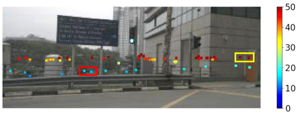
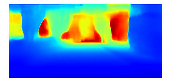
![[Uncaptioned image]](https://cdn.awesomepapers.org/papers/e43483e6-4b90-4266-9b94-a36753be7199/x1.png) |
![[Uncaptioned image]](https://cdn.awesomepapers.org/papers/e43483e6-4b90-4266-9b94-a36753be7199/x2.png) |
![[Uncaptioned image]](https://cdn.awesomepapers.org/papers/e43483e6-4b90-4266-9b94-a36753be7199/x3.png) |
| (a) | (b) | (c) |
1 Introduction
We seek to incorporate automotive radar as a contributing sensor to D scene estimation. While recent work fuses radar with video for the objective of achieving improved object detection [4, 33, 26, 32, 35], here we aim for pixel-level fusion of depth estimates, and ask if fusing video with radar can lead to improved dense depth estimation of a scene.
Up to the present, outdoor depth estimation has been dominated by LiDAR, stereo, and monocular techniques. The fusion of LiDAR and video has lead to increasingly accurate dense depth completion [17]. At the same time, radar has been relegated to the task of object detection in vehicle’s Advanced Driver Assistance Systems (ADAS) [30]. However, phased array automotive radar technologies have been advancing in accuracy and discrimination [14]. Here we investigate the suitability of using radar instead of LiDAR for the task of dense depth estimation. Unlike LiDAR, automotive radars are already ubiquitous, being integrated in most vehicles for collision warning and similar tasks. If successfully fused with video, radar could provide an inexpensive alternative to LiDARs for D scene modeling and perception. However, to achieve this, attentive algorithm design is required in order to overcome some of the limitations of radar, including coarser, lower resolution, and sparser depth measurements than typical LiDARs.
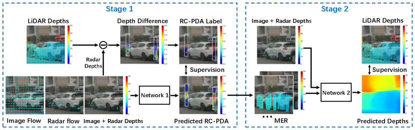
This paper proposes a method to fuse radar returns with image data and achieve depth completion; namely a dense depth map over pixels in a camera. We develop a two-stage algorithm. The first stage builds an association between radar returns and image pixels, during which we resolve some of the uncertainty in projecting radar returns into a camera. In addition, this stage is able to filter occluded radar returns and “densify” the projected radar depth map along with a confidence measure for these associations (see Fig. 1 (a,b)). Once a faithful association between radar hits and camera pixels is achieved, the second stage uses a more standard depth completion approach to combine radar and image data and estimate a dense depth map, as in Fig. 1(c).
A practical challenge to our fusion goal is the lack of public datasets with radar. KITTI [12], the dataset used most extensively for LiDAR depth completion, does not include radar and nor do the Waymo [43] or ArgoVerse [5] datasets. The main exception is nuScenes [3] and the small Astyx [31] which have radar, but unfortunately do not include a dense, pixel-aligned depth map as created by Uhrig et al. [45]. Similarly, the Oxford Radar Robot Car dataset [1] includes camera, LiDAR and raw radar data, but no annotations are available for scene understanding. As a result, all experiments of this work will use the nuScenes dataset along with its annotations. However, we find single LiDAR scans insufficient to train depth completion, and so accumulate scans to build semi-dense depth maps for training and evaluating depth completion.
The main contributions of this work include:
-
•
Radar-camera pixel depth association that upgrades the projection of radar onto images and prepares a densified depth layer.
-
•
Enhanced radar depth that improves radar-camera depth completion over raw radar depth.
-
•
LiDAR ground truth accumulation that leverages optical flow for occluded pixel elimination, leading to higher quality dense depth images.
2 Related Work
Radar for ADAS
Frequency Modulated Continuous Wave radars are inexpensive and all-weather, and have served as the key sensor for modern ADAS. Ongoing advances are improving radar resolution and target discrimination [14], while convolutional networks has been used to add discriminative power to radar data, moving beyond target detection and tracking to include classifying road environments [24, 41], and seeing beyond-line-of-sight targets [40]. Nevertheless, the low spatial resolution of radar means that the D environment, including object shape and classification, are only coarsely obtained. A key path to upgrading the capabilities of radar is through integration with additional sensor modalities [30].
Radar-camera fusion
Early fusion of video with radar, such as [21], relied on radar for cueing image regions for object detection or road boundary estimation [19], or used optical flow to improve radar tracks [11]. With the advent of deep learning, much more extensive multi-modal fusion has become possible [9]. However, to the best of our knowledge, no prior work has conducted pixel-level dense depth fusion between radar and video.
Radar-camera object detection
Object detection is a key task in D perception [2]. There has been significant recent interest in combining radar with video for improved object detection. In [4], ResNet blocks [15] are used to combine both color images and image-projected radar returns to improve longer-range vehicle detection. In [26], an FFT applied to raw radar data generates a polar detection array which is merged with a bird’s eye projection of the camera image, and targets are estimated with a single shot detector [27]. In [32], features from both images and a bird’s-eye representation of radar enter a region proposal network that outputs bounding boxes [42]. An alternative model for radar hits is a m vertical line on the ground plane which is projected into the image plane by [35], and combined with VGG blocks to classify vehicle detections at multiple scales. Our work differs fundamentally from these methods in that our goal is dense depth estimation, rather than object classification. But we do share similarity in radar representation: we project radar hits into an image plane. However, the key novelty in our work is that we learn a neighborhood pixel association model for radar hits, rather than relying on projected circles [4] or lines [35].
LiDAR-camera depth completion
Our task of depth estimation has the same goal as LiDAR-camera depth completion [20, 36, 48, 17, 16]. However, radar is far sparser than LiDAR and has lower accuracy, which makes these methods unsuitable for this task. Our radar enhancement stage densifies the projected radar depths, followed by a more traditional depth completion architecture.
Monocular depth estimation
Monocular depth inference may be supervised by LiDAR or self-supervised. Self-supervised methods learn depth by minimizing photometric error between images captured by cameras with known relative positions. Additional constrains such as semantics segmentation [50, 37], optical flow [18, 46], surface normal [49] and proxy disparity labels [47] improve performance. Recently, self-supervised PackNet [13] has achieved competitive results. Supervised methods [10, 8] include continuous depth regression and discrete depth classification. BTS [23] achieves state of the art by improving upsampling via additional plane constraints, and more recently [38] combines supervised and self-supervised methods. Our goal is not monocular depth estimation, but rather to improve what is achievable from monocular depth estimation through fusion with radar.
3 Method
While there are a variety of data-spaces in which radar can be fused with video, the most natural, given our objective of estimating a high resolution depth map, is in the image space. But this immediately presents a problem: to which pixel in an image does a radar pixel belong? By radar pixel we mean a simple point projection of the estimated D radar hit into the camera. The nuScenes dataset [3] provides extrinsic and intrinsic calibration parameters needed to map the radar point clouds from the radar coordinates system to the egocentric and camera coordinate systems.
Assuming that the actual depth of the image pixel is the same as the radar pixel depth turns out to be fairly inaccurate. We describe some of the problems with this model, and then propose a new pixel association model. We present a method for building this new model and show its benefit by incorporating it into radar-camera depth completion. Fig. 2 shows the diagram of the proposed method.
3.1 Radar Hit Projection Model
Single-row scanning automotive radars can be modeled as measuring points in a plane extending usually horizontally (relative to the vehicle platform) in front of the vehicle, as in [4]. While radars can measure accurate depth, often the depth they give when projected into a camera is incorrect, as can be seen in the examples in Fig. 3. An important source of this error is the large width of radar beams which means that the hits extend well beyond the assumed horizontal plane. In other words, the height of measured radar hits is inaccurate [34].
In addition to beam width, another source of projected point depth difference is occlusion caused by the significant baseline between radars on the grill, and cameras on the roof or driver mirror. Further, these depth differences only increase when radar hits are accumulated over a short interval, and thus more opportunity for occlusions.
In addition to pixel association errors, we are faced with the problem that automotive radars generate far sparser depth scans than LiDAR. There is typically a single row of returns, rather than anywhere up to rows in LiDAR, and the azimuth spacing of radar returns can be an order of magnitude greater than LiDAR. This sparsity significantly increases the difficulty in depth completion. One solution is to accumulate radar pixels over a short time interval, and to account for their D position using both ego-motion and radial velocity. Nevertheless, this accumulation introduces additional pixel association errors (in part from not having tangential velocity) and more opportunities for occlusions.
 |
 |
| (a) | (b) |
3.2 Radar-Camera Pixel Depth Association
In using radar to aid depth estimation we face the problem of determining which, if any, point in the image does a radar return correspond to? This radar pixel to camera pixel association is a difficult problem, and we do not have ground truth to determine this. Thus we reformulate this problem slightly to make it more tractable.
The new question we ask is: “Which pixels in the vicinity of the projected radar pixel have the same depth of that radar return?” We call this Radar-Camera Pixel Depth Association: RC-PDA or simply PDA. It is a one-to-many mapping, rather than one-to-one mapping, and has four key advantages. First, we do not need to distinguish between many good but ambiguous matches and rather can return many pixels with the same depth. This simplifies the problem. Second, by associating the radar return with multiple pixels, our method explicitly densifies the radar depth map, which facilitates the second stage of full-image depth estimation. Third, our question simultaneously addresses the occlusion problem; if there are no nearby pixels with that depth, then the radar pixel is automatically inferred to be occluded. Fourth, we are able to leverage a LiDAR-based ground-truth depth map as the supervision, rather than a difficult-to-define “ground truth” pixel association. Fig. 4 illustrates image depths obtained from raw radar projections and RC-PDA around each radar pixel. It shows the height errors of measured radar points and how some hits visible to the radar are occluded from the camera.
3.2.1 RC-PDA Model
We model RC-PDA over a neighborhood around the projected radar pixel in the color image. At each radar pixel we define a patch around the radar location and seek to classify each pixel in this patch as having the same depth or not as the radar pixel, within a predetermined threshold. A similar connectivity model has been used for image segmentation [22]. Radar pixels and the patches around them are illustrated in Figs. 5(a) and (b), respectively.
 |
 |
 |
| (a) | (b) | (c) |
The connection to each pixel in a neighborhood has elements, and can be encoded as an -channel RC-PDA which we label , where . Here is the radar pixel coordinate, and the ’th neighbor has offset from . Now the label for is 1 if the neighboring pixel has the same depth as radar pixel and 0 otherwise. More precisely, if is the difference between radar pixel depth, , and the neighboring LiDAR pixel depth, , and is the relative depth difference, then:
| (1) |
We note that labels are only defined when there is both a radar pixel at and a LiDAR depth . We define a binary weight to be when both conditions are satisfied and otherwise. During training we minimize the weighted binary cross entropy loss [22] between labels and predicted RC-PDA:
| (2) |
The network output, , is passed through a Sigmoid to obtain , the estimated RC-PDA.
Our network thus predicts a RC-PDA confidence in a range of to representing the probability that each pixel in this patch has the same depth as the radar pixel. This prediction also applies to the image pixel at the same coordinates as the radar pixel, , as like other pixels, the depth at this image pixel may differ from the radar depth for a variety of reasons, including those illustrated in Fig. 4.
3.3 From RC-PDA to MER
The RC-PDA gives the probability that neighboring pixels have the same depth as the measured radar pixel. We can convert the radar depths along with predicted RC-PDA into a partially filled depth image plus a corresponding confidence as follows. Each of neighbors to a given radar pixel is given depth and confidence . If more than one radar depth is expanded to the same pixel, the radar depth with the maximum RC-PDA is kept. The expanded depth is represented as with confidence . Now many of the low-confidence pixels will have incorrect depth. Instead of eliminating low-confidence depths, we convert this expanded depth image into a multi-channel image where each channel is given depth if its confidence is greater than a channel threshold , where and is the total number of channels of the enhanced depth. The result is a Multi-Channel Enhanced Radar (MER) image with each channel representing radar-derived depth at a particular confidence level (see Fig. 5(c)).
Our MER representation for depth can correctly encode many complex cases of radar-camera projection, a few of which are illustrated in Fig. 4. These cases include when radar hits are occluded and no nearby pixels have similar depth. They also include cases where the radar pixel is just inside or just outside the boundary of a target. In each case, those nearby pixels with the same depth as the radar can be given the radar depth with high confidence, while the remaining neighborhood pixels are given low confidence, and their depth are specified on separate channels of the MER.
The purpose of using multiple channels for depths with different confidences in MER is to facilitate the task of Network in Fig. 2 in performing the dense depth completion. High confidence channels give the greatest benefit, but low confidence channels may also provide useful data. In all cases they densify the depth beyond single radar pixels, easing the depth completion task.
3.4 Estimating RC-PDA
We next select inputs to Network in Fig. 2 from which it can learn to infer the RC-PDA. These are the image, the radar pixels with their depths as well as the image flow and the radar flow from current to a neighboring frame. Here we briefly explain the intuition for each of these.
The image provides scene context for each radar pixel, as well as object boundary information. The radar pixels provide depth for interpreting the context and a basis for predicting the depth of nearby pixels. As radar is very sparse, we accumulate radar from a short time history, seconds, and transform it into the current frame using both ego-motion and the radial velocity similar to that done in [35].
Now a pairing of image optical flow and radar scene flow provides an occlusion and depth difference cue. For static objects, the optical flow should exactly equal radar scene flow, when the pixel depth is the same as radar pixel depth. Conversely, radar pixels that are occluded from the camera view will have different scene flow from the optical flow of a static object occluding them (Fig. 6). Similarly, objects moving radially will have consistent flow. By providing flow, we expect that Network will learn to leverage flow similarity in predicting RC-PDA for each radar pixel.
 |
 |
 |
| (a) Radar depth | (b) Optical flow | (c) Radar flow |
 |
 |
 |
| (a) | (b) | (c) |
3.5 LiDAR-based Supervision
To train both the RC-PDA and the final dense depth estimate, we use a dense ground truth depth. This is because, as illustrated in Fig. 7, training with sparse LiDAR leads to significant artifacts. We now describe how we build a semi-dense depth image from LiDAR scans.
3.5.1 LiDAR Accumulation
To our knowledge, there is no existing public dataset specially designed for depth completion with radar. Thus we create a semi-dense ground truth depth from nuScenes dataset, a public dataset with radar data and designed for object detection and segmentation. We use the -ray LiDAR as depth label and notice that the sparse depth label generated from a single frame will lead to a biased model predicting depth with artifacts, i.e., only predictions for pixels with ground truth are reasonable. Thus, we use semi-dense LiDAR depth as label, which is created by accumulating multiple LiDAR frames. With ego motion and calibration parameters, all static points can be transformed to destination image frame. Moving points are compensated by bounding box poses at each frame, which are estimated by interpolating bounding boxes provided by nuScenes in key frames.
3.5.2 Occlusion Removal via Flow Consistency
When a foreground object occludes some of the accumulated LiDAR points, the resulting dense depth may include depth artifacts as the occluded pixels appear in gaps in the foreground object. KITTI [45] takes advantages of the depth from stereo images to filter out such occluded points. As no stereo images are available in nuScenes, we propose detecting and removing occluded LiDAR points based on optical-scene flow consistency.
 |
 |
 |
| (a) LiDAR depth | (b) Optical flow | (c) LiDAR flow |
The scene flow of LiDAR points, termed LiDAR flow, is computed by projecting LiDAR points into two neighboring images and measuring the change in their coordinates. On moving objects, the point’s positions are corrected with the object motion. On static visible objects, LiDAR flow will equal optical flow, while on occluded surfaces LiDAR flow is usually different from the optical flow at the same pixel, see Fig. 8. We calculate optical flow with [44] pretrained on KITTI, and measure the difference between the two flows at the same pixel via the norm of their difference. Points with flow difference larger than a threshold are discarded as occluded points. Fig. 9 shows an example of using flow consistency to filter out occluded LiDAR depths.
 |
 |
| (a) | (b) |
3.5.3 Occlusion Removal via Segmentation
Flow-based occluded pixel removal may fail in two cases. When there is little to no parallax, both optical and scene flow will be small, and their difference becomes not measurable. This occurs mostly at long range or along the motion direction. Further, LiDAR flow on moving objects can in some cases be identical to the occluded LiDAR flow behind it. In both of these cases flow consistency is insufficient to remove occluded pixels from the final depth estimate.
 |
 |
| (a) Car image | (b) Semantic seg. & bound. box |
 |
 |
| (c) Depth before filtering | (d) Depth after filtering |
To solve this problem, we use a combination of D bounding boxes and semantic segmentation to remove occluded points appearing on top of objects. First, accurate pixel region of an instance is determined by the intersection of D bounding box projection and semantic segmentation. The maximum depth of bounding box corners is used to decide whether LiDAR points falling on the object are on it or behind it. Points within the semantic segmentation and closer than this maximum distance are kept, while points in the segmentation and behind the bounding box are filtered out as occluded LiDAR points. Fig. 10 shows an example of removing occluded points appearing on vehicle instances. We use a semantic segmentation model [6] pre-trained with CityScape [7] to segment vehicle pixels.
 |
 |
 |
 |
 |
 |
 |
 |
 |
 |
 |
 |
 |
 |
 |
 |
 |
 |
 |
 |
 |
 |
 |
 |
 |
 |
 |
 |
 |
 |
 |
 |
 |
 |
|
| (a) | (b) | (c) | (d) | (e) | (f) | (g) |
3.6 Algorithm Summary
We propose a two-stage depth estimation process, as in Fig. 2. The Stage estimates RC-PDA for each radar pixel, which is transformed into our MER representation as detailed in Sec. 3.3 and fed into Stage which performs conventional depth completion. Both stages are supervised by the accumulated dense LiDAR, with pixels not having a LiDAR depth given zero weight. Network uses an encoder-decoder network with skip connections similar to U-Net [39] and [28] with details in supplementary material.
4 Experimental Results
Dataset We train and test on a subset of images from the nuScenes dataset [3], including , and samples for training, validation and testing, respectively. The data are collected with moving ego vehicle so flow calculation described in Sec. 3.5.2 can be applied. The depth range for training and testing is - meters. Resolutions of inputs and outputs are . As described in Sec. 3.5, we build semi-dense depth images by accumulating LiDAR pixels from subsequent frames and previous frames (sampled every other frame), and use these for supervision.
Implementation details For parameters, we use m and for Eq. 1. In Sec. 3.5.2 we use to decide flow consistency. MER has channels with to set as , , , , and , respectively. At Stage , we use a U-Net with levels of resolutions and output channels, corresponding to pixels in a rectangle neighborhood with size and . As the radar points are typically on the lower part of image, to fully leveraging the neighborhood, the neighborhood center is below the rectangle center with pixel above, pixels below and pixels on left and right to provide more space for radar points to extend upwards. At Stage , we employ two existing depth completion architectures, [29] and [25], originally designed for LiDAR-camera pairs.
 |
 |
 |
 |
 |
 |
 |
 |
| (a) | (b) | (c) | (d) |
4.1 Visualization of Predicted RC-PDA
The predicted RC-PDA and estimated depths from Stage [29] are visualized in Fig. 11. Column (a) shows the raw radar pixels plotted on images and often include occluded radar pixels. Column (b) shows how image pixels are associated with different radar pixels according to their maximum RC-PDA. Radar pixels and their associated neighboring pixels are marked with the same color. Notice in column (c) that RC-PDA is high within objects and decreases after crossing boundaries. Occluded radar depth are mostly discarded as their predicted RC-PDA is low. In column (e), the dense depths predicted from MER are improved over predictions from (g) raw radar and/or (f) monocular. For example, in Row of Fig. 11, our predicted pole depth in (e) has better boundaries than monocular-only in (f), and monocular plus raw radar in (g). How we achieve this can be intuitively understood by comparing raw radar in (a) with our MER in (d), the output of Stage . While raw radar has many incorrect depths, MER selects correct radar depths and extends these depths along the pole and background, enabling improved final depth inference.
4.2 Accuracy of MER
To be useful in improving radar-camera depth completion, the enhanced radar depth in the vicinity of radar points should be better than alternatives. We compare the depth error of the MER in regions where RC-PDA is , with a few baseline methods and results are shown in Tab. 1. The enhanced radar depth from Stage improves over not only raw radar depth but also depth estimates from Stage using monocular as well as monocular plus radar. In comparison, Stage keeps the accuracy of the enhanced radar depth when using it for depth completion. The depth error for raw radar depth is very large since many of them are occluded and far behind foreground. About of radar points in the test frames have a maximum RC-PDA smaller than in their neighborhood and are discarded as occluded points. Further, Fig. 13 shows the depth error and per-image average area of expanded depth from MER channels, respectively. It shows, as confidence increases, higher RC-PDA corresponds to higher accuracy and smaller expanded areas.
| Network | Input | MAE | Abs Rel | RMSE | RMSE log |
|---|---|---|---|---|---|
| Image | |||||
| Ma et al. [29] | Image, radar | ||||
| Image, radar, MER | |||||
| Li et al. [25] | Image, radar | ||||
| Image, radar, MER | |||||
| None | MER | ||||
| Radar |
 |
4.3 Comparison of Depth Completion
To evaluate effectiveness of the enhanced radar depth in depth completion, we compare the depth error with and without using MER as input for Network , and show performance in Tabs. 2 and 3. The results show that including radar improves depth completion over monocular, while using our proposed MER further improves the accuracy of depth completion for the same network.
Qualitative comparisons between depth completion [29] with and without using MER are shown in Fig. 12. This shows improvement from MER in estimating object depth boundaries including close objects (such as the traffic sign on the bottom image) and far objects.
5 Conclusion
Radar-based depth completion introduces additional challenges and complexities beyond LiDAR-based depth completion. A significant difficulty is the large ambiguity in associating radar pixels with image pixels. We address this with RC-PDA, a learned measure that associates radar hits with nearby image pixels at the same depth. From RC-PDA we create an enhanced and densified radar image called MER. Our experiments show that depth completion using MER achieves improved accuracy over depth completion with raw radar. As part of this work we also create a semi-dense accumulated LiDAR depth dataset for training depth completion on nuScenes.
Acknowledgement This work was supported by the Ford-MSU Alliance.
References
- [1] Dan Barnes, Matthew Gadd, Paul Murcutt, Paul Newman, and Ingmar Posner. The Oxford radar RobotCar dataset: A radar extension to the Oxford RobotCar dataset. In IEEE International Conference on Robotics and Automation, pages 6433–6438, 2020.
- [2] Garrick Brazil, Gerard Pons-Moll, Xiaoming Liu, and Bernt Schiele. Kinematic 3D object detection in monocular video. In European Conference on Computer Vision, pages 135–152, 2020.
- [3] Holger Caesar, Varun Bankiti, Alex H Lang, Sourabh Vora, Venice Erin Liong, Qiang Xu, Anush Krishnan, Yu Pan, Giancarlo Baldan, and Oscar Beijbom. nuScenes: A multimodal dataset for autonomous driving. In IEEE Conference on Computer Vision and Pattern Recognition, pages 11621–11631, 2020.
- [4] Simon Chadwick, Will Maddern, and Paul Newman. Distant vehicle detection using radar and vision. In IEEE International Conference on Robotics and Automation, pages 8311–8317, 2019.
- [5] Ming-Fang Chang, John Lambert, Patsorn Sangkloy, Jagjeet Singh, Slawomir Bak, Andrew Hartnett, De Wang, Peter Carr, Simon Lucey, Deva Ramanan, et al. Argoverse: 3D tracking and forecasting with rich maps. In IEEE Conference on Computer Vision and Pattern Recognition, pages 8748–8757, 2019.
- [6] Bowen Cheng, Maxwell D Collins, Yukun Zhu, Ting Liu, Thomas S Huang, Hartwig Adam, and Liang-Chieh Chen. Panoptic-DeepLab: A simple, strong, and fast baseline for bottom-up panoptic segmentation. In IEEE Conference on Computer Vision and Pattern Recognition, pages 12475–12485, 2020.
- [7] Marius Cordts, Mohamed Omran, Sebastian Ramos, Timo Rehfeld, Markus Enzweiler, Rodrigo Benenson, Uwe Franke, Stefan Roth, and Bernt Schiele. The Cityscapes dataset for semantic urban scene understanding. In IEEE Conference on Computer Vision and Pattern Recognition, pages 3213–3223, 2016.
- [8] Raul Diaz and Amit Marathe. Soft labels for ordinal regression. In IEEE Conference on Computer Vision and Pattern Recognition, pages 4738–4747, 2019.
- [9] Di Feng, Christian Haase-Schuetz, Lars Rosenbaum, Heinz Hertlein, Claudius Glaeser, Fabian Timm, Werner Wiesbeck, and Klaus Dietmayer. Deep multi-modal object detection and semantic segmentation for autonomous driving: Datasets, methods, and challenges. IEEE Transactions on Intelligent Transportation Systems, 2020.
- [10] Huan Fu, Mingming Gong, Chaohui Wang, Kayhan Batmanghelich, and Dacheng Tao. Deep ordinal regression network for monocular depth estimation. In IEEE Conference on Computer Vision and Pattern Recognition, pages 2002–2011, 2018.
- [11] Fernando Garcia, Pietro Cerri, Alberto Broggi, Arturo de la Escalera, and José María Armingol. Data fusion for overtaking vehicle detection based on radar and optical flow. In IEEE Intelligent Vehicles Symposium, pages 494–499. IEEE, 2012.
- [12] Andreas Geiger, Philip Lenz, and Raquel Urtasun. Are we ready for autonomous driving? the KITTI vision benchmark suite. In IEEE Conference on Computer Vision and Pattern Recognition, pages 3354–3361, 2012.
- [13] Vitor Guizilini, Rares Ambrus, Sudeep Pillai, Allan Raventos, and Adrien Gaidon. 3D packing for self-supervised monocular depth estimation. In IEEE Conference on Computer Vision and Pattern Recognition, pages 2485–2494, 2020.
- [14] Jurgen Hasch. Driving towards 2020: Automotive radar technology trends. In IEEE MTT-S International Conference on Microwaves for Intelligent Mobility, pages 1–4, 2015.
- [15] Kaiming He, Xiangyu Zhang, Shaoqing Ren, and Jian Sun. Deep residual learning for image recognition. In IEEE Conference on Computer Vision and Pattern Recognition, pages 770–778, 2016.
- [16] Saif Imran, Xiaoming Liu, and Daniel Morris. Depth completion with twin-surface extrapolation at occlusion boundaries. In IEEE Conference on Computer Vision and Pattern Recognition, 2021.
- [17] Saif Imran, Yunfei Long, Xiaoming Liu, and Daniel Morris. Depth coefficients for depth completion. In IEEE Conference on Computer Vision and Pattern Recognition, pages 12438–12447, 2019.
- [18] Joel Janai, Fatma Guney, Anurag Ranjan, Michael Black, and Andreas Geiger. Unsupervised learning of multi-frame optical flow with occlusions. In European Conference on Computer Vision, pages 690–706, 2018.
- [19] Florian Janda, Sebastian Pangerl, Eva Lang, and Erich Fuchs. Road boundary detection for run-off road prevention based on the fusion of video and radar. In IEEE Intelligent Vehicles Symposium, pages 1173–1178, 2013.
- [20] Maximilian Jaritz, Raoul De Charette, Emilie Wirbel, Xavier Perrotton, and Fawzi Nashashibi. Sparse and dense data with CNNs: Depth completion and semantic segmentation. In International Conference on 3D Vision, pages 52–60, 2018.
- [21] Zhengping Ji and Danil Prokhorov. Radar-vision fusion for object classification. In International Conference on Information Fusion, pages 1–7, 2008.
- [22] Michael Kampffmeyer, Nanqing Dong, Xiaodan Liang, Yujia Zhang, and Eric P Xing. ConnNet: A long-range relation-aware pixel-connectivity network for salient segmentation. IEEE Transactions on Image Processing, 28(5):2518–2529, 2018.
- [23] Jin Han Lee, Myung-Kyu Han, Dong Wook Ko, and Il Hong Suh. From big to small: Multi-scale local planar guidance for monocular depth estimation. arXiv preprint arXiv:1907.10326, 2019.
- [24] Seongwook Lee, Byeong-Ho Lee, Jae-Eun Lee, and Seong-Cheol Kim. Statistical characteristic-based road structure recognition in automotive FMCW radar systems. IEEE Transactions on Intelligent Transportation Systems, 20(7):2418–2429, 2018.
- [25] Ang Li, Zejian Yuan, Yonggen Ling, Wanchao Chi, Chong Zhang, et al. A multi-scale guided cascade hourglass network for depth completion. In IEEE Winter Conference on Applications of Computer Vision, pages 32–40, 2020.
- [26] Teck-Yian Lim, Amin Ansari, Bence Major, Daniel Fontijne, Michael Hamilton, Radhika Gowaikar, and Sundar Subramanian. Radar and camera early fusion for vehicle detection in advanced driver assistance systems. In Machine Learning for Autonomous Driving Workshop at Conference on Neural Information Processing Systems, 2019.
- [27] Wei Liu, Dragomir Anguelov, Dumitru Erhan, Christian Szegedy, Scott Reed, Cheng-Yang Fu, and Alexander C Berg. SSD: Single shot multibox detector. In European Conference on Computer Vision, pages 21–37, 2016.
- [28] Fangchang Ma, Guilherme Venturelli Cavalheiro, and Sertac Karaman. Self-supervised sparse-to-dense: self-supervised depth completion from LiDAR and monocular camera. In IEEE International Conference on Robotics and Automation, pages 3288–3295, 2019.
- [29] Fangchang Ma and Sertac Karaman. Sparse-to-dense: Depth prediction from sparse depth samples and a single image. In IEEE International Conference on Robotics and Automation, pages 4796–4803, 2018.
- [30] Enrique Marti, Miguel Angel de Miguel, Fernando Garcia, and Joshue Perez. A review of sensor technologies for perception in automated driving. IEEE Intelligent Transportation Systems Magazine, 11(4):94–108, 2019.
- [31] Michael Meyer and Georg Kuschk. Automotive radar dataset for deep learning based 3D object detection. In European Radar Conference, pages 129–132, 2019.
- [32] Michael Meyer and Georg Kuschk. Deep learning based 3D object detection for automotive radar and camera. In European Radar Conference, pages 133–136, 2019.
- [33] Ramin Nabati and Hairong Qi. RRPN: Radar region proposal network for object detection in autonomous vehicles. In IEEE International Conference on Image Processing, pages 3093–3097, 2019.
- [34] Ramin Nabati and Hairong Qi. CenterFusion: Center-based radar and camera fusion for 3D object detection. In IEEE Winter Conference on Applications of Computer Vision, pages 1527–1536, 2021.
- [35] Felix Nobis, Maximilian Geisslinger, Markus Weber, Johannes Betz, and Markus Lienkamp. A deep learning-based radar and camera sensor fusion architecture for object detection. In Sensor Data Fusion: Trends, Solutions, Applications, pages 1–7, 2019.
- [36] Jiaxiong Qiu, Zhaopeng Cui, Yinda Zhang, Xingdi Zhang, Shuaicheng Liu, Bing Zeng, and Marc Pollefeys. DeepLiDAR: Deep surface normal guided depth prediction for outdoor scene from sparse LiDAR data and single color image. In IEEE Conference on Computer Vision and Pattern Recognition, pages 3313–3322, 2019.
- [37] Pierluigi Zama Ramirez, Matteo Poggi, Fabio Tosi, Stefano Mattoccia, and Luigi Di Stefano. Geometry meets semantics for semi-supervised monocular depth estimation. In Asian Conference on Computer Vision, pages 298–313, 2018.
- [38] Haoyu Ren, Aman Raj, Mostafa El-Khamy, and Jungwon Lee. SUW-Learn: Joint supervised, unsupervised, weakly supervised deep learning for monocular depth estimation. In IEEE Conference on Computer Vision and Pattern Recognition Workshops, pages 750–751, 2020.
- [39] Olaf Ronneberger, Philipp Fischer, and Thomas Brox. U-Net: Convolutional networks for biomedical image segmentation. In International Conference on Medical Image Computing and Computer Assisted Intervention, pages 234–241, 2015.
- [40] Nicolas Scheiner, Florian Kraus, Fangyin Wei, Buu Phan, Fahim Mannan, Nils Appenrodt, Werner Ritter, Jurgen Dickmann, Klaus Dietmayer, Bernhard Sick, et al. Seeing around street corners: Non-line-of-sight detection and tracking in-the-wild using Doppler radar. In IEEE Conference on Computer Vision and Pattern Recognition, pages 2068–2077, 2020.
- [41] Heonkyo Sim, The-Duong Do, Seongwook Lee, Yong-Hwa Kim, and Seong-Cheol Kim. Road environment recognition for automotive FMCW radar systems through convolutional neural network. IEEE Access, 8:141648–141656, 2020.
- [42] Karen Simonyan and Andrew Zisserman. Very deep convolutional networks for large-scale image recognition. In International Conference on Learning Representations, 2015.
- [43] Pei Sun, Henrik Kretzschmar, Xerxes Dotiwalla, Aurelien Chouard, Vijaysai Patnaik, Paul Tsui, James Guo, Yin Zhou, Yuning Chai, Benjamin Caine, et al. Scalability in perception for autonomous driving: Waymo open dataset. In IEEE Conference on Computer Vision and Pattern Recognition, pages 2446–2454, 2020.
- [44] Zachary Teed and Jia Deng. RAFT: Recurrent all-pairs field transforms for optical flow. In European Conference on Computer Vision, pages 402–419, 2020.
- [45] Jonas Uhrig, Nick Schneider, Lukas Schneider, Uwe Franke, Thomas Brox, and Andreas Geiger. Sparsity invariant CNNs. In International Conference on 3D Vision, pages 11–20, 2017.
- [46] Sudheendra Vijayanarasimhan, Susanna Ricco, Cordelia Schmid, Rahul Sukthankar, and Katerina Fragkiadaki. SfM-Net: Learning of structure and motion from video. arXiv preprint arXiv:1704.07804, 2017.
- [47] Jamie Watson, Michael Firman, Gabriel J Brostow, and Daniyar Turmukhambetov. Self-supervised monocular depth hints. In IEEE International Conference on Computer Vision, pages 2162–2171, 2019.
- [48] Yan Xu, Xinge Zhu, Jianping Shi, Guofeng Zhang, Hujun Bao, and Hongsheng Li. Depth completion from sparse LiDAR data with depth-normal constraints. In IEEE International Conference on Computer Vision, pages 2811–2820, 2019.
- [49] Zhenheng Yang, Peng Wang, Wei Xu, Liang Zhao, and Ramakant Nevatia. Unsupervised learning of geometry with edge-aware depth-normal consistency. arXiv preprint arXiv:1711.03665, 2017.
- [50] Shengjie Zhu, Garrick Brazil, and Xiaoming Liu. The edge of depth: Explicit constraints between segmentation and depth. In IEEE Conference on Computer Vision and Pattern Recognition, pages 13116–13125, 2020.