Quasinormal modes, temperatures and greybody factors of black holes in a generalized Rastall gravity theory
Abstract
We introduce a modification in the energy-momentum conservation violating Rastall’s theory of gravity and obtain a Reissner-Nordström-type black hole solution in spacetime surrounded by a cloud of strings and charge fields. We examine the horizons of the black hole along with the influence of the parameters of the model on it. The scalar quasinormal modes (QNMs) of oscillations of the black hole are also computed using the 6th order WKB approximation method. It is seen that the Rastall parameter and the newly introduced energy-momentum tensor trace parameter as well as the charge parameter and strings field parameter influence the amplitude and damping of the QNMs. From the metric function, we obtain the temperature of the black hole and study the effects of the four model parameters , , and on the temperature. We then examine the greybody factors associated with the black hole and the corresponding total absorption cross-section for it. It is seen that the modification we introduced in the Rastall theory has a drastic effect on various properties of the black hole and may lead to interesting outcomes in future when better detection techniques will be available with the LISA and the Einstein Telescope.
I Introduction
The theory of General Relativity (GR) was endowed with the revolutionary description of gravity, which undoubtedly has appeared as the major milestone in the field of modern astrophysics and cosmology. The two of the most significant predictions made by GR have been observationally verified most recently: the detection of gravitational waves (GWs) from the binary black hole system merger by the LIGO-Virgo collaboration [1, 2, 3, 4, 5, 6] and the first images of the black hole M87* by the Event Horizon Telescope (EHT) [7, 8, 9, 10, 11, 12]. These two observational verifications increase the importance of the theory even today. Moreover, GR has been tested in the post-Newtonian levels to a high precession viz., by the light deflection, Shapiro time delay and perihelion advance of Mercury [13, 14, 15]. Confirmation of the validity of GR has also been inferred from the Hulse-Taylor binary pulsar timing array data which matched the GR predicted GWs damping to high accuracy [16, 17, 18]. All these reasons are more than sufficient to state that GR is indeed a successful theory of gravity.
However, GR is afflicted with some issues. The theory is non-renormalizable in
the high energy regime [19]. Also in the infrared regime, there are
deviations from experimental findings like the accelerated expansion of
the Universe [20, 21] and the dark matter sector [22]. That is, we
cannot explain the accelerated expansion of the Universe and features that
indicate the hidden matter content of the Universe with this theory. To
overcome these issues, many theories of gravity have been proposed, the most
common class of which are the Modified Theories of Gravity (MTGs) (see
[23, 24] and references therein). In these theories, either the matter
side or the curvature side of the general Einstein field equations are
modified to mitigate these issues. CDM model [25] represents
the simplest amongst the matter-modified theories or the usually known dark
energy models [26], and theory [27] represents one
of the simplest among the spacetime geometry-modified theories or the commonly
referred MTGs. Some other MTGs include Rastall gravity
[28, 29, 30, 31, 32, 33, 34], gravity [35], gravity
[36, 37, 38, 39, 40, 41, 42], gravity [43] etc.
In 1972, P. Rastall proposed his theory of gravity which gained popularity
eventually, as this theory was capable of predicting observational results
like galactic rotation curves [44] and accelerated expansion of the
Universe [45]. However, the point to be noted is that this theory is not
derived from an action principle approach which is one of the drawbacks of the
theory. In this theory, the energy-momentum conservation law is modified and
the covariant derivative of the energy-momentum tensor is taken to be
proportional to the covariant derivative of the Ricci scalar . This theory
recovers GR in the regime of zero background curvature. Thus, Rastall’s theory
is a generalization of GR in a sense. However, Visser in his paper
[33] argued that Rastall gravity (RG) is equivalent to GR and that RG
does not provide any new insights compared to GR. A number of counterarguments
have been advanced which restate that RG is a more general theory of gravity
and it includes GR as a special case. In Ref. [46], the authors
stated clearly that any metric theory including gravity can be
transformed into a GR-like form but that does not imply that the theories are
equivalent. In fact, they provide compelling arguments in support of RG.
Moreover, in Ref. [47], Darabi et al. have pointed out deviations
of RG from GR based on cosmological observations. Similarly, in
Ref. [48], authors investigate compact stellar objects using
modified Rastall teleparallel gravity. Recently, Hansraj et
al. [49] reinforced the claim of Darabi and his team.
Moreover this theory provides predictions regarding the age of the Universe
[50] and the Hubble parameter [50]. This theory can justify the
gravitational lensing process [51] and also the existence of traversable
wormhole solutions has been shown recently [52]. In one work, the
authors, in the context of Rastall gravity, studied the gravitational collapse
of a homogeneous perfect fluid [53]. In another recent work, the authors
studied ABG-type black holes in Rastall gravity surrounded by a string’s cloud
in the presence of non-linear electrodynamic sources [31]. In the
paper [54] the authors studied the neutron star for a
realistic equation of state under the framework of Rastall gravity [54].
Similarly, the authors of the paper [55] have studied the thermodynamic
properties along with Joule-Thomson expansion and the optical properties of
the black hole surrounded by quintessence, under the framework of Rastall
gravity. In Ref. [56] authors introduced a generalised form of the
Rastall gravity and studied the compact objects in this framework.
The motivation to choose Rastall theory over other modified gravity
theories comes from the fact of the simplicity of field equations of RG as
compared to other theories. Moreover, RG is capable of handling modern
observational constraints and various avenues of theoretical research have
been persued in recent times considering this framework.
Black holes are frequently studied with a surrounding field that impacts their
properties to a good extent. In 2003, Kiselev studied black holes surrounded
by the quintessence [57] and since then many research works have been
published with such fields surrounding the black holes
[30, 31, 32, 58, 59, 60, 61, 62, 63, 64, 65, 66]. P. Letelier studied black holes surrounded by
clouds of strings [64]. Recently, different surrounding fields like dark
matter fields or dark energy fields have been considered. Heydarzade and
Darabi considered the Kiselev-like charged/uncharged black hole solutions
surrounded by a perfect fluid in the framework of Rastall gravity [30].
In another work, the authors implemented GUP corrections into the black hole solution
surrounded by quintessence matter [58]. They studied the QNMs and
thermodynamic properties of the black hole. Chen et. al. [66] studied the Hawking radiation of a d-dimensional black hole
surrounded by quintessence fields. The existence of Nariai black holes for
some specific parameters has been shown in Ref. [67]. Thermodynamics of
the quantum-corrected Schwarzschild black hole surrounded by quintessence has
been studied recently in Ref. [68].
As indicated earlier, the emission of GWs is an interesting phenomenon related
to black holes, which can convey important information regarding black
holes [24, 69, 70, 71]. QNMs represent the
complex frequencies of oscillations associated with the emission of GWs from
perturbed massive objects in the Universe [31, 32, 58, 69, 70, 71, 72, 73].
The real part of it gives the amplitude and the imaginary part represents
the damping associated with the GWs. QNMs have been studied extensively
in the literature in different scenarios like charged, spinning or simple
stationary black holes with different types of surrounding fields implementing
different theories of gravity (MTGs) apart from GR [31, 32, 58, 69, 70, 71, 72, 73].
The greybody factor, which specifies the transmission behaviour of a black
hole is an important quantum property of black holes. This factor has been
studied extensively in different gravity theories
[32, 74, 75, 76, 77, 78, 79]. The authors of Ref. [74] studied the
Bardeen de Sitter (dS) black holes for scalar perturbation and calculated the
greybody factors for the black holes. In Ref. [75], the authors have
examined electromagnetic and gravitational perturbations of the Bardeen
dS black hole and calculated the QNMs along with the
greybody factor. They also examined the total absorption cross-section for
the metric. Konoplya et. al. [76] presented the recipe for computing
the QNMs and greybody factors for black holes using the higher order
WKB approximation method and discussed some issues as well as advantages of
this method. The greybody factors have been studied for massive scalar fields
in dRGT gravity for AdS and dS cases in Ref. [77]. Authors in Ref. [32] studied the Reissner-Nordström (RN)-type AdS/dS black holes
with the surrounding quintessence field. In Ref. [78], the authors studied the greybody factors and Hawking radiation of
black holes considering 4D Einstein-Gauss-Bonnet gravity. In another work, the
authors studied the QNMs and greybody factors of black holes in
symmergent gravity [79].
In this present work, we modify the energy-momentum conservation condition of
GR making the covariant derivative of the energy-momentum tensor proportional
to the derivative of and , where is the trace of the energy-momentum
tensor. This model is inspired by Ref. [56] where the authors have
studied the effect of such a modification in Rastall theory on compact objects.
With this modified Rastall theory we intend to study the behaviour of the
charged black hole, i.e. RN black hole solution surrounded by
a Maxwell field and a cloud of strings, specifically its QNMs,
thermodynamics temperature and the greybody factor. Motivated by
previous studies as mentioned earlier we choose the source sustaining the
black hole solution, i.e. a solution surrounded by a Maxwell field and a
cloud of strings. The idea of black holes surrounded by a Maxwell field comes
naturally as a black hole has a high probability of interaction with its
surrounding environment by means of phenomena such as accretion. It is a
physical possibility that a black hole can be charged. The strings field is
motivated by string theory which proposes strings as the most fundamental unit
of matter. This has been implemented in literature [31] and following
this, we implement the same in the black holes’ environment in our study in
the sense that the surrounding mass of an interacting black hole may be in
the form of clouds of strings due to the extreme nature of black holes’
immediate spacetime. The black hole solution obtained by us is unique and has
scope for studying black hole shadows, accretion disk, gravitational lensing
along with other properties.
This paper is organised as follows. In Section II, we discuss the
Rastall theory and the modification imposed. We also solve the field equations
after considering a charged background together with string clouds. In
Section III, we give a brief account of the QNMs of oscillations of the
black hole and compute the complex frequencies for the black hole in the
particular setup. In Section IV, we compute the thermodynamic
temperature associated with the black hole for various values of the model
parameters and analyse them. In Section V, we study the greybody
factors and absorption coefficient associated with the black hole. Finally, in
section VI, we present the concluding remarks and future directions.
II Field equations of modified rastall theory
GR demands that the covariant derivative of the energy-momentum tensor should vanish, that is Rastall modified this conservation condition, generalising it to the form:
| (1) |
where represents the Rastall parameter. This Rastall form of modification of the conservation condition is based on the fact that variation of energy-momentum of spacetime should depend on the corresponding variation of the curvature of the spacetime. Nevertheless, it is also possible that the pattern of variation of the energy-momentum of spacetime depends on the energy-momentum content of spacetime in addition to its curvature variation. Considering this aspect in mind, here we introduce a further modification in the conservation condition as follows:
| (2) |
where is a constant parameter associated with , which measures the deviation of the theory from Rastall’s original form. Using the above equations, one can deduce the field equations for the modified Rastall gravity as
| (3) |
Assuming , we can rewrite the above field equations in an elegant form as
| (4) |
The trace of the equation (4) gives
| (5) |
For our work, we will stick to the spherically symmetric black hole metric ansatz [31],
| (6) |
where . Defining the Rastall tensor , the following non-vanishing components of the modified field equations (4) can be obtained as
| (7) | ||||
| (8) | ||||
| (9) | ||||
| (10) |
Here, prime denotes derivative with respect to . The expression of the Ricci scalar is obtained as
| (11) |
We assume that the spherically symmetric spacetime surrounding the black hole is characterized by the presence of an electric charge field and a string’s cloud field. Hence, the total energy-momentum tensor of the considered spacetime is defined as
| (12) |
In this relation is the Maxwell tensor having the form:
| (13) |
where denotes the black hole charge parameter. The other term represents the surrounding string’s cloud field which in simplified form can be written as [31]
| (14) |
where is the string’s cloud density parameter. To derive the explicit form of this parameter, we make use of the equations (2), (5) and (14) to get the following differential equation:
| (15) |
The above equation can be solved and the following solution for is obtained:
| (16) |
where is the constant of integration, which is associated with the string’s density parameter. We impose the condition on that to respect the weak energy condition. Moreover, one interesting point to note from equation (16) is that for the physical consistency, we should have , otherwise its equality to zero will lead to divergence of string density. This condition leads to setting a constraint on the possible values of for a given value of . For instance, if we choose , we see that the value of should be . Finally, we are in a situation to write the Rastall field equations in a complete form as in the following:
| (17) | ||||
| (18) |
Solving equations (17) and (18), the general solution for the metric function of the black hole is found as
| (19) |
where is the string parameter as it is directly associated with the density of the string field. This string parameter is constrained by the weak energy condition as . The black hole metric function (19) is the RN black hole solution surrounded by a cloud of strings in the modified Rastall theory. It is to be noted at this point that a feasible black hole solution should satisfy the energy conditions, especially the weak energy condition (WEC). Thus we need to check the consistency of solution (19) with the WEC. The criteria for satisfaction of WEC are as follows [80]:
| (20) |
| (21) |
Here represents the mass function that can be extracted from the metric solution and has the following form.
| (22) |
Calling these three functions as , and respectively, we have shown in Figure 1 the obeyance of the WEC by the solution (19) for the parameter values we mostly use in this work. It should also be noted that violation of WEC has been observed for higher values of parameters.


Returning to equation (19), in the limit and going to zero, we recover the RN solution and also for , we recover the Schwarzschild black hole solution. We can also recover the well-known RN-AdS solution from the metric solution by properly substituting values of the constants. This shows that the metric solution obtained here is general and encompasses many well-known black hole solutions. The behaviour of the metric function (19) is shown in Figure 2 with various values of the model parameters. Here, we can see that there are three horizons for the black hole metric. It is observed that the outermost horizon is impacted mostly by string parameter and hence it is called the string horizon. The first plot shows the metric function variation for different values of the string parameter . It is seen from the curves that variation in the values of does not affect the single inner horizon of the black hole but there is a visible impact on the outer horizon, which we may refer to as the string horizon. With the increase in , the string horizon gradually decreases as shown in the plot. The second plot shows the metric function variation for various values of charge parameter . Here, it is seen that has negligible influence on the string horizon but mainly influences the two inner horizons. As increases, the dip of the metric curve decreases and finally, we get a critical value of beyond which there is no inner horizon as can be seen from the plot. The third plot shows the behaviour of the metric function for various values of the Rastall parameter . It is clear that has negligible influence on the inner horizons but mainly impacts the outer string horizon. As can be seen, with higher values of , the outer horizon radius decreases gradually. Also, we plot the metric function for different values of . As can be seen from the fourth plot, with an increase in , the outer horizon radius increases. Further, it is to be noted that as seen from the first plot of the figure, the metric function behaves very differently than the Schwarzschild one except in the overlapping region of the horizon radius.


Now we focus on the determination of the black hole’s QNMs of oscillations for which we shall use the 6th order WKB approximation method. This method is the most widely used and trusted method of calculating QMNs and provides a mechanism for error estimation as well as higher order calculations for better accuracy. It matches the results of other analytical and numerical methods like the asymptotic iteration method, continued fraction method and time domain analysis method [32, 69, 75, 81].
III WKB approximation method for calculating QNMs
The most important step for computing the QNMs of the black hole defined by the metric function (19) with the scalar perturbation using the WKB approximation method is to obtain the potential associated with the black hole metric. For which we are to perturb the black hole spacetime with a probe that minimally couples with a scalar field described by the equation of motion [58],
| (23) |
Here we consider a massless scalar field so that the right hand side of the above equation reduces to zero. In this setup, it is convenient to express field in spherical polar form as [58]
| (24) |
where we represent the radial part of the wave by and represents the spherical harmonics. is the oscillation frequency of the time component of the wave, which corresponds to the frequency of QNMs of oscillation of the black hole solution. Implementing equation (24) in equation (23), one can obtain the following Schrödinger-type equation:
| (25) |
where the new variable is the well-known tortoise coordinate, defined as
| (26) |
and the effective black hole potential for the setup is obtained from the usual from [58]:
| (27) |
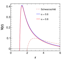
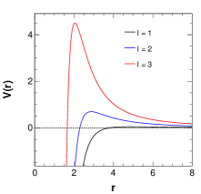
Here denotes the multipole number. Figure (3) shows the behaviour of this potential for different values of model parameters , , and along with different values of the multipole number . It is seen that for all model parameters, the potential is significantly different from that for the Schwarzschild case, especially in the peak region of the potential. Moreover, for higher values the peak of the potential is substantially higher than that for the smaller and it also shifts towards the smaller horizon radius.
In order to have physical consistency, we impose boundary conditions on the radial part of the wave function at the horizon and infinity as follows:
| (30) |
where and are the integration constants. In consideration of the above criteria, we calculate the QNM frequencies following the Refs. [58, 69, 70, 71]. In the following figures, we plot the QNM frequencies for the black hole with variations in the model parameters to show their impact on the amplitude and damping of the QNMs.
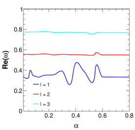
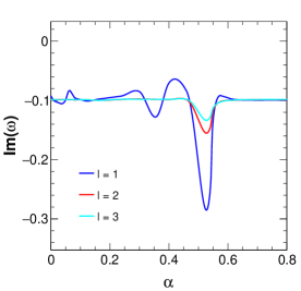
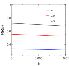
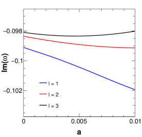
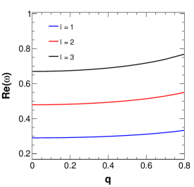
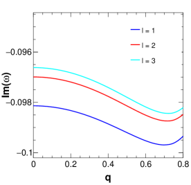
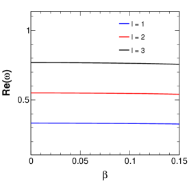
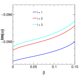
Figure 4 shows the variation of amplitude and damping of QNMs with variation in the parameter . It is seen that there are random oscillatory behaviours in both the real and imaginary parts of the QNMs for values of . For values of , the QNM frequencies show the non-oscillatory stable behaviour. Moreover, the oscillatory behaviour of QNMs for the said range of values of reduces with the increase in values of . This oscillatory behaviour of QNMs signifies the unstable nature of the black hole solution for that particular range of values of , and this also supports our earlier inference on the possible values of for the physical consistency. Because of these in our rest of the study, we consider the value of . Figure 5 shows the variation of the amplitude and damping of the QNMs with variation in the string parameter for three values of . From the figure, it is clear that with increasing , the amplitude of the QNM frequency decreases in such a way that the decrease is very minimal for lower and noticeable for higher . The damping, on the other hand, shows a drastic increase with increasing values, but for higher values of such as , the damping increases slightly and again decreases with increasing values. Figure 6 shows the variation of the QNMs with charge . The first plot of this figure shows the variation of the amplitude with , showing that with increasing charge values, the amplitude also increases. It is also noteworthy that higher multipole also results in higher amplitude values. The damping is mostly higher for smaller values and the variation of damping with respect to increases with increasing charge values up to . After this, there is a drastic decrease in damping as further increases showing the gradually decreasing difference of damping due to different values. Figure 7 represents the variation of QNMs with Rastall parameter , where we can see that the amplitude of the QNMs decreases with very slowly. Although this is not very clear from the figure, the tabular form of QNM frequencies (Table 1) clearly shows this trend. The damping decreases with increasing for the various values of as shown in the plot.
The QNMs for the black hole for various combinations of model parameters have been shown in Table 1, where we also show the calculated approximate errors associated with the 6th order WKB method. The process of error estimation has been adopted from [76] where the authors have suggested the formula,
| (31) |
Here represents the error associated with the 6th order WKB value of QNMs, and respectively means the 7th and 5th order QNM values. It is noteworthy that the WKB method produces reliable results for the regime only and its accuracy increases for higher as is evident from our table also. For , multipoles and are chosen and QNMs along with errors associated are shown in this Table 1. The first four sections in the table are for . In the first section, we keep , and fixed and change to see its effect on the QNMs. It is clear that the amplitude or the real part of QNMs decreases with increasing and a similar trend is also seen in the imaginary part or the damping part. The error estimation is around . The second section shows the variation in while keeping , and fixed. Here, we can see that with an increase in , the amplitude increases while the damping increases initially but later decreases for higher , with error estimation about . In the third section, we fix , and and vary the string parameter . We observe that the amplitude decreases while damping increases with an increase in . The estimated error is about . In the fourth section, we vary the and fix the other parameters. It is seen that both the amplitude as well as damping decreases with increasing . Here, we have an error estimation of about . A Similar setup is presented in the lower sections but with . Here the almost same trend is seen as in the case of but with higher QNM amplitudes, which is almost twice that for the case. In this case, the magnitude of damping is almost equal to that for the earlier case. The error estimation in this case decreases to . Thus it is quite clear that increasing the multipole number leads to more accuracy in WKB results. As a future scope, we can compare various other numerical and analytical methods of calculating QNMs for our particular black hole in modified Rastall gravity, surrounded by clouds of strings.
| Multipole | 6th order WKB QNMs | |||||||
|---|---|---|---|---|---|---|---|---|
| 0.319038 - 0.101938i | ||||||||
| 0.309857 - 0.098262i | ||||||||
| 0.290292 - 0.093340i | ||||||||
| 0.277566 - 0.090237i | ||||||||
| 0.80 | 0.304581 - 0.099204i | |||||||
| 0.80 | 0.321046 - 0.099692i | |||||||
| 0.80 | 0.333653 - 0.099347i | |||||||
| 0.80 | 0.351315 - 0.097390i | |||||||
| 0.80 | 0.304581 - 0.099204i | |||||||
| 0.80 | 0.296683 - 0.100816i | |||||||
| 0.80 | 0.285134 - 0.102889i | |||||||
| 0.80 | 0.258318 - 0.103706i | |||||||
| 0.70 | 0.322953 - 0.105406i | |||||||
| 0.75 | 0.320730 - 0.103206i | |||||||
| 0.80 | 0.319038 - 0.101938i | |||||||
| 0.90 | 0.316019 - 0.100356i | |||||||
| 0.80 | 0.525770 - 0.099130i | |||||||
| 0.80 | 0.514233 - 0.095527i | |||||||
| 0.80 | 0.485430 - 0.090238i | |||||||
| 0.80 | 0.466354 - 0.086931i | |||||||
| 0.80 | 0.470181 - 0.098794i | |||||||
| 0.80 | 0.501907 - 0.099424i | |||||||
| 0.80 | 0.525770 - 0.099130i | |||||||
| 0.80 | 0.558772 - 0.097247i | |||||||
| 0.80 | 0.502511 - 0.098143i | |||||||
| 0.80 | 0.488420 - 0.098703i | |||||||
| 0.80 | 0.470181 - 0.098794i | |||||||
| 0.80 | 0.432185 - 0.096708i | |||||||
| 0.70 | 0.527277 - 0.101960i | |||||||
| 0.75 | 0.526872 - 0.100228i | |||||||
| 0.80 | 0.525770 - 0.099130i | |||||||
| 0.90 | 0.522562 - 0.097652i |
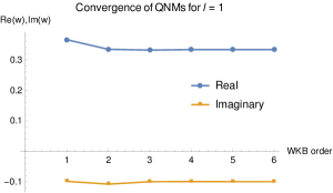
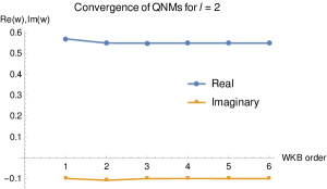
We also plot the convergence of the QNMs of various WKB orders in Figure 8. We have shown the convergence of QNMs up to 6th WKB order calculation.
The quality factor is a good means of showcasing the strength of a wave of oscillations versus its damping. It is basically a dimensionless quantity and demonstrates how under-damped the wave is. The more the quality factor, the more will be the strength of oscillation compared to damping. Mathematically we express the quality factor by the formula:
| (32) |
We plot the quality factor of QNMs for our black hole solution with respect to charge , string parameter and Rastall parameter and parameter in Figure 9. It is clear from the figure that the quality factor decreases with an increase in and while the quality factor increases gradually with an increase in . Concerning , this factor first increases slowly, then decreases minutely with an increase in . This means that the black hole system becomes overdamped with increasing values of and .


IV Temperature of the black hole and its characteristics
The temperature of a black hole is an important characteristic, which we want to analyse for our model. From the metric function (19), we can get the event horizon radius for our black hole by the condition , where implies the horizon radius of the black hole. In the general Schwarzschild case, we encounter a comparatively simple expression but in our case, we cannot get an analytical expression directly for the horizon radius because of the complicated nature of the metric function and hence we shall follow some other methods accordingly. To this end, we first derive the surface gravity of the black hole using the relation [31],
| (33) |
From the numerical calculations we encounter three horizons in the case of our metric for a specific set of values of model parameters (see Figure 2). The innermost horizon is called the inner or Cauchy horizon, the next horizon is referred to as the outer or event horizon and the last one is the outermost or the string horizon respectively. Using the expression of the surface gravity, we can derive the Hawkings temperature by using the relation [31],
| (34) |
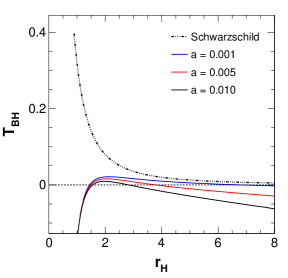
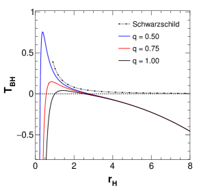
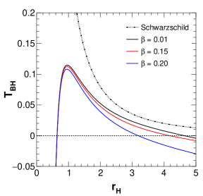
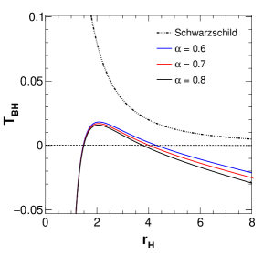
Here horizon radius has three values, viz., , and which are respectively the inner horizon or Cauchy horizon, the event horizon and the string horizon. We follow Ref. [34] to plot Hawking temperature with respect to which encompasses all three horizons. Before that, we numerically compute the Hawking temperature and its variation with changing values of model parameters along with the horizon radius values, which are shown in Table 2. In this table, we show the variation of horizon radii and temperature for various values of model parameters. It is clear from this table that and parameters influence the second and third horizon, while not impacting the first horizon. Parameter impacts both the first and second horizon while not impacting third horizon. Finally, affects the third horizon, meaning that with increasing , the third horizon radius increases and temperature decreases.
| 0.001 | 0.6 | 0.01 | 0.80 | 0.4000 | 1.0200 | 6.3136 | -0.59683 | 0.0372 | -0.0447 |
| 0.010 | 0.6 | 0.01 | 0.80 | 0.4000 | 1.7316 | 2.2235 | -0.59687 | 0.0187 | -0.0222 |
| 0.010 | 0.7 | 0.01 | 0.80 | 0.4000 | 1.6105 | 5.5805 | -0.59686 | 0.0360 | -0.0328 |
| 0.001 | 0.6 | 0.01 | 0.90 | 0.5641 | 1.4364 | 6.3211 | -0.21801 | 0.0336 | -0.0451 |
| 0.001 | 0.6 | 0.10 | 0.90 | 0.5641 | 1.4382 | 19.3570 | -0.21810 | 0.0335 | -0.0093 |
Figure 10 shows the variation of black hole temperature with horizon radius for different values of the parameters. The first plot represents temperature versus horizon radius for different values of the string parameter . It is observed that with an increase in , the graph deviates more from the ideal Schwarzschild case towards the negative temperature side and for , the temperature drops down to negative values. Similar is the case with higher horizon radius values where the temperature gradually goes towards the negative side. The second plot shows the variation of temperature with horizon radius for various values of charge and the third plot is shown for various values of the parameter . Similarly, the fourth plot shows temperature variation curves for different values. It is clear that for all the scenarios, at a very small horizon radius, the black hole becomes ultracold with negative temperatures which doesn’t sound very physical but this has been encountered in research work before [31, 82]. Similarly, the temperature of black holes with increasingly higher horizon radii becomes increasingly more negative.
V Greybody factors and absorption cross section
In this section, we analyse the transmission coefficient or the greybody factor for the black hole [32, 75, 76, 77, 78, 79]. The greybody factor tells us about the amount of radiation near the black hole that is trapped or reflected by the black hole. The greybody factor gives an idea of the probability for the outwards traveling wave to reach an observer at infinity, without getting absorbed or the probability of an incoming wave getting absorbed by the black hole. The study of reflection coefficient and transmission coefficient (greybody factor) is not new, a lot of researchers have already studied these coefficients in various scenarios. The greybody factor for the scalar perturbation in the Bardeen-de Sitter black hole setup has been studied in detail in [74]. More recently, the greybody factor for the Bardeen-de Sitter black hole has been studied for electromagnetic as well as gravitational perturbations [75]. The reflection and transmission of the wave hitting the barrier potential can be of the following form [75]:
| (35) | ||||
| (36) |
where and are reflection and transmission coefficients respectively, and functions of . The condition of the conservation of probability demands that These two coefficients can be obtained from the WKB approximation approach as [32, 75, 76, 77, 78, 79].
| (37) | ||||
| (38) |
where parameter can be determined as [32, 75],
| (39) |
Expression for the WKB correction terms can be found in
Ref. [71]. Here represents the effective potential maximum and the
double dash is for the double derivative with respect to . We plot the
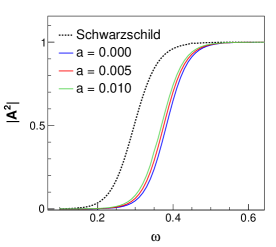
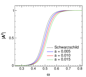
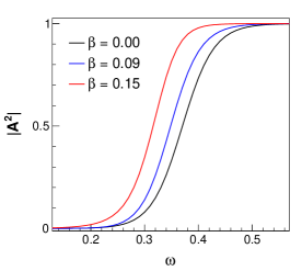
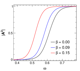
greybody factors (square of the transmission coefficient) versus for
different values of the model parameters in Figures 11, 12,
13 and 14. Figure 11 shows the greybody factor versus
for varying values of the string parameter with and
taking the multipole (left) and (right). It is clear
that for higher values of , value slightly increases
starting from the smaller frequency . The changes become more visible
for as shown in the figure (right plot). An increase in the value of the
transmission coefficient suggests that there is less scattering of the wave
back from the barrier with an increasing value of . However, at very small
and large values of , the parameter does not have any noticeable effect.
Moreover, we see that although the pattern of variation of greybody factor of
the black hole is similar to the Schwarzschild black hole, the pattern is
shifted to low frequency side for , whereas it is shifted to the high
frequency side for
higher values in comparison to that for the Schwarzschild black hole.
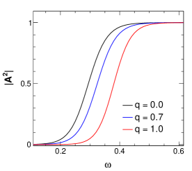
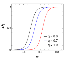
Figure 12 shows the same plots but for the varying charge with
keeping the same value. Here, we see that with an increase in
charge, the greybody factor decreases and thus scattering increases. The effect
gets amplified on increasing multipole from 1 to 2. Figure 13 shows a
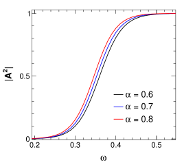
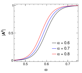
similar plot for varying with keeping the same value of . Here
it is seen that higher values result in higher values of
greybody factor and hence less scattering. Figure 14 shows the greybody
plots for variation in values. Similar to the previous cases, here
also greybody factor increases with increasing values.
The absorption cross-section of the black hole corresponding to the transmission coefficient can be computed using the relation [75],
| (40) |


In Figure 15, we show the total absorption cross-section for the black hole as a function of with values of the model parameters as shown in the caption. Here we consider the summation of multipoles upto 8 terms in the expression. It is clear that the cross-section value increases abruptly with to a maximum value and then saturates for some range of and finally decreases gradually for higher values. The plot can be superficially divided into three regions. The first region is the increasing region, which corresponds with the increasing transmission coefficient plots that we have shown. The second part is the oscillating part due to many multimodes considered in finding . The third region shows a power-law type falloff which is due to saturation of transmission coefficient value to 1, and hence when is higher valued, then . Moreover, it is seen that increases with increasing values of and , while it decreases with increasing and values. The effects of and on are appreciable with the domination as the most significant.
VI Conclusion
In this work, we modify the Rastall gravity theory and compute the corresponding black hole metric with a cloud of strings field surrounding the black hole. The effects of the parameters of the theory on the horizon of the black hole have been analysed. The string parameter and the gravity model parameters influence the outermost horizon while the charge impacts the inner horizons. We then compute the scalar QNMs for the black hole using the 6th order WKB approximation method and observe the dependence of the amplitude and damping on various parameters. It is observed that the amplitude decreases while the damping increases (for there is a slight change in the pattern) with an increase in the string parameter . It is seen that with an increase in , the amplitude increases, whereas the damping increases at the beginning but later decreases. For , it is observed that the amplitude decreases very minutely, while damping decreases noticeably with increasing values. Moreover, it found that for the physical consistency the values of the parameter should be greater than . Thus for higher values of the parameter, the amplitude and damping of QNMs are seen to be decreased with increasing values (see Table 1). We estimate the approximate errors associated with the WKB calculations as shown in the Table 1.
Further, the convergence of QNMs for various orders of the WKB method has been checked. We plot the quality factor of the emission of QNMs to estimate the strength of amplitude over damping. Then we plot the temperature of the black hole versus the horizon radius for different model parameters. In all the cases, the temperature plots show a peak for smaller values of horizon radius and then go towards negative values for very small and higher values of the horizon radius, indicating ultracold black hole formation possibility in such cases. We compute the greybody factors associated with the black hole metric and plot the same versus frequency for different model parameters. We see that for larger values of , the transmittance increases more rapidly for . For smaller values of , the transmittance is more. It is also seen that transmittance increases with increase in and values. In all four cases, it is seen that the saturation of transmittance value occurs more quickly for compared to multipole value. We also compute the total absorption cross-section () and plotted it with respect to for variations in different model parameters. It is found that the higher the parameters and are, the more the absorption cross-section. However, the reverse is observed for the cases of and parameters. The parameters and affect significantly the absorption cross-section.
It needs to be mentioned that efforts are going on to improve the efficiency and the sensitivity of the existing GW detectors. Moreover, new detectors of GWs like LISA [83, 84] and the Einstein Telescope [85] will come up with a significant improvement in detection sensitivity, which will allow one to constrain our model and other theories of gravity very effectively and help to eliminate redundant propositions. We believe that more work needs to be done in this direction and with time, as we have more and more accurate information regarding different properties of black holes, especially of the QNMs, it will be more convenient to validate various MTGs, which is one of the sought after intentions in this arena. As a future scope, we can study the electromagnetic and gravitational QNMs of the black hole for our particular setup. Further, the black hole shadow data can also be used to perform a constraining study on various parameters of the theory. Furthermore, one can also perform the classical tests of GR, namely precession of planetary orbits, Shapiro time delay and gravitational bending of light to suggest some constraints on various parameters of the theory. Other possible scopes of the obtained black hole solution include gravitational lensing study and accretion physics. These are some of the possible future prospects of the work.
Acknowledgements
UDG is thankful to the Inter-University Centre for Astronomy and Astrophysics (IUCAA), Pune, India for awarding the Visiting Associateship of the institute.
References
- [1] B. P. Abbott et al., Observation of Gravitational Waves from a Binary Black Hole Merger, Phys. Rev. Lett. 116, 061102 (2016).
- [2] B. P. Abbott et al., Observation of Gravitational Waves from a 22-Solar-Mass Binary Black Hole Coalescence, Phys. Rev. Lett. 116, 241103 (2016).
- [3] B. P. Abbott et al., Observation of Gravitational Waves from a Binary Neutron Star Inspiral, Phys. Rev. Lett. 119, 161101 (2017).
- [4] B. P. Abbott et al., Observation of a Binary-Black-Hole Coalescence with Asymmetric Masses, Phys. Rev. D 102, 043015 (2020).
- [5] R. Abbott et al., Observation of Gravitational Waves from Two Neutron Star–Black Hole Coalescences, ApJL 915, L5 (2021).
- [6] R. Abbott et al., Search for continuous gravitational wave emission from the Milky Way center in O3 LIGO-Virgo data, Phys. Rev. D 106, 042003 (2022).
- [7] Event Horizon Telescope Collaboration et al., First M87 Event Horizon Telescope Results. I. The Shadow of the Supermassive Black Hole, APJL 875, L1 (2019).
- [8] Event Horizon Telescope Collaboration et al., First M87 Event Horizon Telescope Results. II. Array and Instrumentation, APJL 875, L2 (2019).
- [9] Event Horizon Telescope Collaboration et al., First M87 Event Horizon Telescope Results. III. Data Processing and Calibration, APJL 875, L3 (2019).
- [10] Event Horizon Telescope Collaboration et al., First M87 Event Horizon Telescope Results. IV. Imaging the Central Supermassive Black Hole, APJL 875, L4 (2019).
- [11] Event Horizon Telescope Collaboration et al., First M87 Event Horizon Telescope Results. V. Physical Origin of the Asymmetric Ring, APJL 875, L5 (2019).
- [12] Event Horizon Telescope Collaboration et al., First M87 Event Horizon Telescope Results. VI. The Shadow and Mass of the Central Black Hole, APJL 875, L6 (2019).
- [13] C. M. Will, The Confrontation between General Relativity and Experiment, Living Reviews in Relativity 17, 4 (2014).
- [14] R. D’Inverno, Introducing Einstein’s Relativity, Oxford University Press (1998).
- [15] R. Cassana, A. Cavalcante, F. P. Poulis and E. B. Santos, An exact Schwarzschild-like solution in a bumblebee gravity model, Phys. Rev. D 97, 104001 (2018).
- [16] T. Damour and J. H. Taylor, Strong-field tests of relativistic gravity and binary pulsars, Phys. Rev. D 45, 1840 (1992).
- [17] N. Yunes and X. Siemens, Gravitational-Wave Tests of General Relativity with Ground-Based Detectors and Pulsar-Timing Arrays, Living Reviews in Relativity 16, 9 (2013).
- [18] M. Maiorano, F. De Paolis and A.A. Nucita, Principles of Gravitational-Wave Detection with Pulsar Timing Arrays, Symmetry 13, 2418 (2021).
- [19] K.S. Stelle, Renormalization of higher-derivative quantum gravity, Phys. Rev. D 16, 953 (1977).
- [20] A. G. Riess et al., Observational Evidence from Supernovae for an Accelerating Universe and a Cosmological Constant, The Astronomical Journal 116, 1009 (1998).
- [21] S. Perlmutter et al., Measurements of and from 42 High-Redshift Supernovae, The Astrophysical Journal 517, 556 (1999).
- [22] N. A. Bahcall, J. P. Ostriker, S. Perlmutter and P. J. Steinhardt, The Cosmic Triangle: Revealing the State of the Universe, Science 284, 5419 (1999).
- [23] S. Shankaranarayanan and J. P. Johnson, Modified theories of gravity: Why, how and what?, Gen. Relativ. Gravit. 54, 44 (2022).
- [24] D. J. Gogoi and U. D. Goswami, A new f (R) Gravity Model and properties of Gravitational Waves in it, EPJC 80, 1101 (2020).
- [25] N. Deruelle and J.-P. Uzan, Relativity in Modern Physics, Oxford University Press (2018).
- [26] S. Weinberg, The Cosmological constant problem, Rev. Mod. Phys. 61, 1 (1989).
- [27] A. de-Felice and S. Tsujikawa, f(R) theories, Living Reviews in Relativity 13, 3 (2010).
- [28] P. Rastall, Generalization of the Einstein Theory, Phys. Rev. D 6, 3357 (1972).
- [29] Y. Heydarzade, H. Moradpour and F. Darabi, Black Hole Solutions in Rastall Theory, Can. J. Phys. 95, 1253 (2017).
- [30] Y. Heydarzade and F. Dahabi, Black hole solutions surrounded by perfect fluid in Rastall theory, Phys. Lett. B 771, 365 (2017).
- [31] D. J. Gogoi, R. Karmakar and U. D. Goswami, Quasinormal modes of nonlinearly charged black holes surrounded by a cloud of strings in Rastall gravity, IJGMMP 20, 235007 (2023).
- [32] D. J. Gogoi, N. Heidari, J. Ǩrǐz and H. Hassanabadi, Quasinormal Modes and Greybody factors of de Sitter Black holes Surrounded by Quintessence in Rastall gravity, Fortschr. Phys. 2024, 2300245.
- [33] M. Visser, Rastall gravity is equivalent to Einstein gravity, Phys. Lett. B 782, 83 (2018).
- [34] X. -C. Cai and Y. -G. Miao, Quasinormal modes and spectroscopy of a Schwarzschild black hole surrounded by a cloud of strings in Rastall gravity, Phys. Rev. D 101, 10423 (2020).
- [35] T. Harko, F. S. N. Lobo, S. Nojiri and S. D. Odinstov, f(R,T) gravity, Phys. Rev. D 84, 024020 (2011).
- [36] P. Sarmah, A. De and U. D. Goswami, Anisotropic LRS-BI Universe with f(Q) gravity theory, Physics of the Dark Universe 40, 101209 (2023).
- [37] A. De, S. Mandal, J. T. Beh, T. H. Loo and P. K. Sahoo, Isotropization of locally symmetricBianchi-I universe in f(Q)-gravity, EPJC 82, 10052 (2022).
- [38] R. Solanki, A. De, S. Mandal and P. K. Sahoo, Accelerating expansion of the universe in modified symmetric teleparallel gravity, Physics of the Dark Universe 36, 101053 (2022).
- [39] D. J. Gogoi, A. Övgün and M. Koussour, Quasinormal Modes of Black holes in gravity, EPJC 83, 700 (2023).
- [40] P. Bhar and J. M. Z. Pretel, Dark energy stars and quark stars within the context of f(Q) gravity, Physics of the Dark Universe 42, 101322 (2023).
- [41] A. Ditta, X. Tiecheng, A. Errehymy, G. Mustafa and S. K. Maurya, Anisotropic charged stellar models with modified Van der Waals EoS in f(Q) gravity, EPJC 83, 254 (2023).
- [42] S. Saklany, N. Pant and B. Pandey, Compact star with coupled dark energy in Karmarkar connected relativistic spacetime, Physics of the Dark Universe 39, 101166 (2023).
- [43] W. A. G. De Moraes and A. F. Santos, Lagrangian formalism for Rastall theory of gravity and Godel-type universe, Gen. Relativ. Gravit. 51, 167 (2019).
- [44] M. Tang, Z. Xu and J. Wang, Observational constraints on Rastall gravity from rotation curves of low surface brightness galaxies, Chinese Physics C 44, 085104 (2020).
- [45] H. Moradpour, Y. Heydarzade, F. Darabi and I. G. Salako, A generalization of the Rastall theory and cosmic eras, EPJC 77, 259 (2017).
- [46] F. Darabi, H. Moradpour, I. Licata, Y. Heydarzade and C. Corda, Einstein and Rastall Theories of Gravitation in comparison, EPJC 78, 25 (2018).
- [47] H. Moradpour, A. Bonila, E. M. C. Abreu and J. A. Neto, Accelerated cosmos in a nonextensive setup, Phys. Rev. D 96, 123504 (2017).
- [48] A. Ditta, X. Tiecheng, G. Mustafa and A. Errehymy, The effect of modified hybrid and logarithmic teleparallel gravity on the interior solutions of compact stars, EPJC 83, 1020 (2023).
- [49] S. Hasnraj, A. Banerjee and P. Channuie, Impact of the Rastall parameter on perfect fluid spheres, Annals of Physics 400, 320 (2019).
- [50] A. S. Al-Rawaf and M. O. Taha, A resolution of the cosmological age puzzle, Phys. Lett. B 366, 69 (1996).
- [51] A.-M. M. Abdel-Rahman and M. H. A. Hashim, Gravitational lensing in a model with non-interacting matter and vacuum energies, Astrophys. Space Sci. 298, 519 (2005).
- [52] H. Moradpour, N. Sadeghnezhad and S. H. Hendi, Traversable asymptotically flat wormholes in Rastall gravity, Can. J. Phys. 95, 1257 (2017).
- [53] A. H. Ziaie, H. Moradpour and S. Ghaffari, Gravitational collapse in Rastall gravity, Phys. Lett. B 793, 276 (2019).
- [54] A. M. Oliveira, H. E. S. Velten, J. C. Fabris and L. Casarini, Neutron stars in Rastall gravity, Phys. Rev. D 92, 044020 (2015).
- [55] D. J. Gogoi, Y. Sekhmani, D. Kalita, N. Gogoi and J. Bora, Joule-Thomson expansion and Optical behaviour of Reissner-Nordstrom-Anti-de Sitter black holes in Rastall gravity surrounded by a Quintessence field, Fortschritte Der Physik 71, 2300010 (2023).
- [56] C. E. Mota, L. C. N. Santos, F. M. da Silva, G. Grams, L. P. Lobo and D. P. Menezes, Generalized Rastall’s gravity and its effects on compact objects, IJMPD 31, 2250023 (2022).
- [57] V. V. Kiselev, Quintessence and black holes, Class. Quantum Grav 20, 1187 (2003).
- [58] R. Karmakar, D. J. Gogoi and U. D. Goswami, Quasinormal modes and thermodynamic properties of GUP-corrected Schwarzschild black hole surrounded by quintessence, IJMPA 37, 2250180 (2022).
- [59] R. Karmakar, D. J. Gogoi and U. D. Goswami, Thermodynamics and shadows of GUP-corrected black holes with topological defects in Bumblebee gravity, Physics of the Dark Universe 41, 101249 (2023).
- [60] M. A. Anacleto, J. A. V Campos, F. A. Brito and E. Passos, Quasinormal modes and shadow of a Schwarzschild black hole with GUP, Annals of Physics 434, 168662 (2021).
- [61] K. Jusufi, Quasinormal Modes of Black Holes Surrounded by Dark Matter and Their Connection with the Shadow Radius, Phys. Rev. D 101, 084055 (2020).
- [62] Í. Güllü and A. Övgün, Schwarzschild-like black hole with a topological defect in bumblebee gravity, Annals of Physics 436, 168721 (2022).
- [63] J. M. Toledo and V. B. Bezerra, The Reissner–Nordstrom black hole surrounded by quintessence and a cloud of strings: Thermodynamics and quasinormal modes, IJMPD 28, 1950023 (2019).
- [64] P. S. Letelier, Clouds of strings in general relativity, Phys. Rev. D 20, 1294 (1979).
- [65] E. Herscovich and M. G. Richarte, Black holes in Einstein–Gauss–Bonnet gravity with a string cloud background, Phys. Lett. B 689, 192-200 (2010).
- [66] S. Chen, B. Wang and R. Su, Hawking radiation in a d-dimensional static spherically symmetric black hole surrounded by quintessence, Phys. Rev. D 77, 124011 (2008).
- [67] S. Fernando, Nariai black holes with quintessence, MPLA 28, 1350189 (2013).
- [68] Md. Shahjalal, Thermodynamics of quantum-corrected Schwarzschild black hole surrounded by quintessence, Nuclear Physics B 940, 63 (2019).
- [69] R. A. Konoplya and A. Zhidenko, Quasinormal modes of black holes: From astrophysics to string theory, Rev. Mod. Phys. 83, 793 (2011).
- [70] R. A. Konoplya, Quasinormal modes of a small Schwarzschild–anti-de Sitter black hole, Phys. Rev. D 66, 044009 (2002).
- [71] R. A. Konoplya, Quasinormal behavior of the D-dimensional Schwarzschild black hole and the higher order WKB approach, Phys. Rev. D 68, 024018 (2003).
- [72] M. Zubair, M. A. Raza and E. Maqsood, Rotating black hole in Kalb-Raymond gravity: Constraining parameters by comparison with EHT observations of Sgr A* and M87*, Physics of the Dark Universe 42, 101334 (2023).
- [73] X. Zhang, M. Wang and J. Jing, Quasinormal modes and late time tails of perturbation fields on a Schwarzschild-like black hole with a global monopole in the Einstein-bumblebee theory, Sci. China Phys. Mech. Astron. 66, 100411 (2023).
- [74] S. Fernando, Bardeen-de Sitter black holes, IJMPD 27, 1750071 (2017).
- [75] S. Dey and S. Chakrabarti, A note on electromagnetic and gravitational perturbations of the Bardeen de Sitter black hole: quasinormal modes and greybody factors, EPJC 79, 504 (2019).
- [76] R. A. Konoplya, A. Zhidenko and A. F. Zinhailo, Higher order WKB formula for quasinormal modes and grey-body factors: recipes for quick and accurate calculations, Class. Quantum Grav. 36, 155002 (2019).
- [77] P. Boonserm, S. Phalungsongsathit, K. Sansuk and P. Wongjun, Greybody factors for massive scalar field emitted from black holes in dRGT massive gravity, EPJC 83, 657 (2023).
- [78] R. A. Konoplya and A. F. Zinhailo, Grey-body factors and Hawking radiation of black holes in 4D Einstein-Gauss-Bonnet gravity, Phys. Lett. B 810, 135793 (2020).
- [79] D. J. Gogoi, A. Övgün and D. Demir, Quasinormal modes and greybody factors of symmergent black hole, Physics of the Dark Universe 42, 101314 (2023).
- [80] L. Balart and E. C. Vagenas, Regular black hole metrics and weak energy condition, Phys. Lett. B 730, 14 (2014).
- [81] H. T. Cho, A. S. Cornell, J. Doukas and W. Naylor, Classical and Quantum Gravity Black hole quasinormal modes using the asymptotic iteration method, Class. Quantum Grav. 27, 155004 (2010).
- [82] M. -I. Park, Can Hawking temperatures be negative?, Phys. Lett. B 663, 259 (2008).
- [83] www.lisamission.org (LISA Consortium).
- [84] www.lisa.nasa.gov (LISA Mission).
- [85] www.et-gw.eu (Einstein Telescope).