Quasinormal Modes and Hawking Radiation Sparsity of GUP corrected Black Holes in Bumblebee Gravity with Topological Defects
Abstract
We have obtained the Generalized Uncertainty Principle (GUP) corrected de Sitter and anti-de Sitter black hole solutions in bumblebee gravity with a topological defect. We have calculated the scalar, electromagnetic and gravitational quasinormal modes for the both vanishing and non-vanishing effective cosmological constant using Padé averaged sixth order WKB approximation method. Apart from this, the time evolutions for all three perturbations are studied, and quasinormal modes are calculated using the time domain profile. We found that the first order and second order GUP parameters and , respectively have opposite impacts on the quasinormal modes. The study also finds that the presence of a global monopole can decrease the quasinormal frequencies and the decay rate significantly. On the other hand, Lorentz symmetry violation has noticeable impacts on the quasinormal frequencies and the decay rate. We have studied the greybody factors, power spectrum and sparsity of the black hole with the vanishing effective cosmological constant for all the three perturbations. The presence of Lorentz symmetry breaking and the GUP parameter decrease, while other GUP parameter and the presence of global monopole increase the probability of Hawking radiation to reach the spatial infinity. The presence of Lorentz violation can make the black holes less sparse, while the presence of a global monopole can increase the sparsity of the black holes. Moreover, we have seen that the black hole area quantization rule is modified by the presence of Lorentz symmetry breaking.
1 Introduction
Although the recent discovery of Gravitational Waves (GWs) has provided strong support to the General Relativity (GR), GR is not renormalizable at UV scale, and hence it describes the gravitation at classical level only. On the other hand, the Standard Model (SM) of particle physics describes particles and other three fundamental interactions at the quantum level. As both GR and SM are the most successful field theories in describing nature, the unification of these two theories is one of the prime pursuits of physicists to describe all fundamental interactions of nature at the quantum level so that we will understand nature to the most deeper level. In the quest of this unification goal, some theories of Quantum Gravity (QG) have already been introduced, whose direct test would be possible only at the Planck scale ( GeV). As this energy scale is far more beyond the reach of current experiments, so direct tests of those QG models are not possible at present and nor will be in the near future. However, there are some effects of QG models, such as the breaking of Lorentz symmetry [1], which may be observed at the current low energy scales [2]. The violation of Lorentz symmetry arises as a possibility in the context of loop quantum gravity, noncommutative field theories, string theory, standard-model extension (SME) etc. Especially, SME is a most general field theoretical framework that includes the fields of SM and GR with the terms in the lagrangian containing information about the Lorentz symmetry violation. The effects of Lorentz symmetry breaking in the gravitational sector of SME were studied in Ref.s [3, 4, 5, 6, 7, 8, 9, 10]. In the case of GWs, the Lorentz violation was studied in Ref.s [11, 12]. The simplest extended gravitational field theories with the spontaneous breaking of Lorentz and diffeomorphism are usually referred to as bumblebee models [1] in which breaking of Lorentz symmetry takes place due to the nonzero vacuum expectation value of a single vector field, known as the bumblebee field. It should be noted that the diffeomorphism violation is always associated with the local Lorentz symmetry violation. Recently a spherically symmetric exact vacuum solution to Einstein field equations in the presence of a spontaneous breaking of Lorentz symmetry due to nonzero vacuum expectation value of the bumblebee field has been obtained in Ref. [2]. This study also explored three classical tests viz., the advance of perihelion, bending of light and Shapiro’s time delay, and showed that corrections from Lorentz violation were present even in the absence of a massive gravitational source and the Lorentz violation background deforms the spacetime. In another study, particle motion in Snyder noncommutative spacetime structures was studied in the presence of Lorentz violation [13].
In a recent study, it was seen that the Lorentz symmetry breaking reduces the greybody factor of black holes in Generalized Uncertainty Principle (GUP) modified bumblebee gravity [14]. In a different study, the photon orbits of Kerr-Sen-like black holes in bumblebee gravity have been investigated, where the authors examined the effects of charge, Lorentz violation parameter and plasma as a dispersive medium [15]. The impact of a topological defect on black holes in bumblebee gravity was studied for the first time in Ref. [16]. In that work, the authors studied the black hole horizon, temperature and the photon sphere extensively and found that the radius of the shadow of black holes increases with an increase in the global monopole parameter. Their study also shows an increasing effect of the deflection angle coming from the Lorentz symmetry breaking parameter and the global monopole. The exact traversable wormhole solution in bumblebee gravity has been obtained in Ref. [17]. In this work, the authors studied the energy conditions of the wormhole and deflection angle of light in explicit form. They found that the bumblebee wormhole solutions support the normal matter wormhole geometries under some certain conditions.
In this work, we shall study the quasinormal modes of GUP corrected black holes in the presence of a topological defect in bumblebee gravity. The quasinormal modes are basically some complex numbers that are related to the emission of GWs from the compact and massive perturbed objects in the universe [18, 19, 20]. The real part of the quasinormal modes is related to the emission frequency, while the imaginary part is connected to its damping. In recent times, the properties of GWs and quasinormal modes of black holes were studied extensively in different modified gravity theories [21, 22, 23, 24, 25, 26, 27, 28, 29, 30, 31, 32, 33]. In Ref. [25], the quasinormal modes of black holes in bumblebee gravity were studied, and it was shown that the Lorentz violation has a significant impact on the quasinormal frequencies. In another recent study, the quasinormal modes of GUP corrected Schwarzschild black holes have been studied and it was seen that the GUP correction could change the quasinormal frequencies and the decay rates of GWs [34]. Being inspired by this study, we have considered the GUP correction in black holes in bumblebee gravity. To have a better comparison, we have considered three different perturbations viz., scalar, electromagnetic and gravitational perturbations to calculate the quasinormal modes of black holes. To obtain the quasinormal modes with higher accuracy, we have implemented Padé averaged WKB approximation method upto sixth order. WKB approximation method provides a good approximation to the quasinormal modes, however, in some cases the method may be deficient to calculate quasinormal modes [35]. For a comparison of our results in time domain, we have studied the time evolution of the perturbation profiles and obtained the quasinormal modes from the time domain analysis. Moreover, we have also studied the aspect of the sparsity of black holes along with greybody factors and Hawking radiation power spectrum. The greybody factor of a black hole is related to the quantum nature of a black hole and it has been widely studied for black holes in different modified theories. In Ref. [36], greybody factors of a black hole in dRGT massive gravity have been studied using rigorous bound and the matching technique. In another work, the nonlinear electrodynamic effects on the black hole shadow, deflection angle, quasinormal modes and greybody factors have been studied in details for a magnetically charged black hole in ‘double-logarithmic’ nonlinear electrodynamics [37]. The greybody factors in black strings have been studied in Ref. [38] in dRGT massive gravity theory where the authors calculated the rigorous bounds on greybody factors. The light rays in a Kazakov-Solodukhin black hole has been studied using Gauss-Bonnet theorem and the greybody bounds have been calculated in details in a recent study [39]. In another important work, quasinormal modes and greybody factors have been also studied in gravity minimally coupled to cloud of strings in dimensions, where the authors found explicit analytical results for decay rate, reflection coefficient, greybody factors and temperature of the black hole [40]. The scalar perturbations of a single-horizon regular black hole has been studied in Ref. [41] where the regular black hole solution was obtained using polymer quantization inspired by loop quantum gravity. The quantum corrections like GUP and non-commutativity are also implemented in black holes to study the thermodynamic behaviours [42]. GUP effects on Hawking temperature of a black hole in warp Dvali-Gabadadze-Porrati (DGP) gravity model have been studied in Ref. [43], where it was found that the mass, angular momentum of vector and scalar particles impact the Hawking temperature of a black hole, and it is connected with the type of the particle emitted from the black hole.
Finally, we perform a study on the area of the black holes with the help of the adiabatic invariance method. Since, the area of black holes is connected with the GW echo [44, 45, 46], entropy spectrum and power spectrum of black holes, we believe the results can be further used to study the impacts of Lorentz violation on different aspects of black holes.
One may note that as the Lorentz symmetry breaking carries the possibilities of beyond standard model physics, it has been an objective of many experimental searches [47, 48]. Apart from bumblebee gravity, such symmetry breaking also arises in different theories including string theory [49] and noncommutative geometry [50]. Such theories with a spontaneously broken symmetry can give rise to different topological defects such as domain wall, cosmic string or monopole solutions etc. Hence, global monopoles are a possibility in bumblebee gravity. In such theories, the topological defects like global monopoles arise during the phase transitions in the early universe via Kibble mechanism [51] and since isolated defects are stable in nature, one may expect that they can still exist in the present universe. The presence of such relics can have some important implications in different aspects of astrophysics and cosmology including structure formation and inflation [52, 53]. In this work, we consider one such type of relics known as global monopole and study its implications in black hole properties such as quasinormal modes, sparsity etc. If one can have some direct or indirect evidence of the existence of such a monopole, they will contribute significantly to the understanding of beyond standard model physics. In other words, such an evidence might represent the first field observed to break Lorentz symmetry, which is not described by the standard model. Apart from the bumblebee field and global monopole, we have considered another ingredient known as GUP. GUP quantum corrections are expected for a black hole in quantum regime or in such length scale. In such an SME theory, GUP has been implemented previously [14]. GUP is based on a momentum-dependent modification in the standard dispersion relation which is conjectured to violate the Lorentz invariance [54]. In another work, it has been shown that the GUP deformation parameter is connected with the violation of Lorentz invariance [55]. Hence for a study of the black holes in bumblebee gravity, inclusion of global monopoles and GUP corrections are necessary for a better understanding of the system.
The work is organized as follows. In the next section 2, we have included a very short review on the field equations of bumblebee gravity and obtained a GUP corrected black hole solution around the global monopole in the bumblebee gravity. The black hole solutions with non-vanishing are obtained in section 3. Here we have discussed the GUP corrected de Sitter and anti-de Sitter black hole solutions. We have obtained the quasinormal modes of black holes in section 4. In this section, we have tried to show the dependency of the quasinormal modes on different parameters of black holes. We have studied the time evolution of three different perturbations in section 5. The possibility of experimental detection of quasinormal modes has been studied in brief in the section 6. The sparsity of black holes is studied in section 7. Finally, we have summarized our results and findings in section 8. Throughout the paper we have considered , where is the Planck length.
2 GUP Corrected Black Hole solutions in Bumblebee Gravity with topological defects
Here we shall briefly review the simplest bumblebee gravity model and then derive the GUP corrected black hole solution in this gravity. In general, bumblebee models are vector or tensor theories that include a potential term which provides nonzero vacuum expectation values in the configuration of the fields. This behaviour of the fields affects the dynamics of other fields coupled to them, maintaining the conservation laws and geometric structures as required by pseudo-Riemannian manifold used in GR [1].
The Lagrangian density of the simplest bumblebee gravity model for the bumblebee field coupled to gravity in a torsion-free spacetime in the presence of the global monopole is given by [2]
| (2.1) |
where , is the cosmological constant, is the bumblebee field with the field strength tensor . is the potential with as a real positive number, for which the spontaneous Lorentz violation takes place and is the coupling constant for a non-minimal gravity-bumblebee field interaction. is basically the Lagrangian density of matter. In our case, we shall consider this to be for the global monopole. First, we shall calculate the field equations of the theory for the vanishing cosmological constant i.e. . The corresponding field equations associated with the theory can be obtained from the Lagrangian (2.1) by varying its action with respect to the metric , which are given by
| (2.2) |
where is the standard Einstein’s tensor. It is seen the energy-momentum tensor part of these field equations is a sum of two tensors: and . The tensor is that part of energy momentum tensor which depends on the bumblebee field and is given by
| (2.3) |
where the prime denotes the derivative with respect to the argument, and the usual matter part for our case is considered to be of the form:
| (2.4) |
Here, the parameter is a constant quantity which is connected to the global monopole charge. The second set of field equations can be obtained by considering the variation of the Lagrangian (2.1) action with respect to the bumblebee field and it is given by
| (2.5) |
where , in which acts as a source term for the bumblebee field, while is the self interaction bumblebee field current.Taking trace of equation (2.2) we get,
| (2.6) |
Now, using equation (2.6) in equation (2.2) we can have,
| (2.7) |
As mentioned above, the potential in the Lagrangian (2.1) generates the nonzero vacuum expectation value for the field since for it is required that
| (2.8) |
One can see that the solution of equation (2.8) gives a nonzero vacuum expectation value where is a vector, which is a function of spacetime coordinates and hence . This nonzero background vector spontaneously violates the Lorentz symmetry. For the completeness it needs to be mentioned that signs in front of decide whether the background field is timelike or spacelike respectively [2, 13, 14, 16, 25]. For a static and spherically symmetric black hole solution with the Lorentz symmetry violation in the bumblebee field we consider the Birkhoff metric as an ansatz:
| (2.9) |
where and are functions of and we fix the bumblebee field in its vacuum expectation value [56], i.e.
| (2.10) |
These lead the radial background field as given by
| (2.11) |
where is the radial component of . Using this component it is possible to write the equation (2.7) as the extended Einstein’s equations in vacuum in the form as
| (2.12) | ||||
| (2.13) |
where the trace of the energy-momentum tensor is given by
| (2.14) |
The components of equation (2.13) can be written explicitly as
| (2.15) | ||||
| (2.16) | ||||
| (2.17) | ||||
| (2.18) |
where . Solving these equations (2.15), (2.16), (2.17) and (2.18) we obtain,
| (2.19) | ||||
| (2.20) |
Thus, with these results the Lorentz symmetry breaking spherically symmetric solution for the field equations can be given as
| (2.21) |
Here, we have chosen where is the mass of the black hole and the global monopole term. The metric (2.21) will give the Lorentz symmetry breaking standard spherically symmetric solution when [2], and the usual Schwarzschild metric for both and .
The prediction of the existence of a minimal length from different approaches of QG such as the black hole physics and the string theory has many important physical implications at very high energy scales. For example, at Planck scale the Schwarzschild radius of the corresponding black hole becomes comparable to the Compton wavelength. Thus the existence of a minimal length demands for the GUP, which is defined as [57, 58, 59, 60, 61]
| (2.22) |
where and are dimensionless positive parameters. It is clear from the above relation that for one can easily recover the Heisenberg’s uncertainty principle, i.e. . Following Ref. [57], we can obtain a bound for the massless particles as
| (2.23) |
which changes the equation (2.22) to
| (2.24) |
where denotes the GUP corrected energy. Assuming and , we can write the above equation (2.24) in terms of mass as the following mass relation:
| (2.25) |
This mass relation leads to the GUP corrected event horizon as given by
| (2.26) |
Finally, the metric for a GUP corrected black hole in the bumblebee gravity with topological defects can be obtained from the metric (2.21) by replacing the black hole mass with the corresponding GUP corrected mass as given by
| (2.27) |
and the event horizon of this black hole would be
| (2.28) |
3 Black holes with non-vanishing
In presence of non-vanishing cosmological constant, the metric functions which satisfy the modified field equations in absence of magnetic monopole are given by [62]
| (3.1) |
and
| (3.2) |
Here the effective cosmological constant. Now, in presence of global monopole, these metric functions are found to be of the form:
| (3.3) |
and
| (3.4) |
Depending on the value of , the above solutions can be classified into anti-de Sitter and de Sitter solutions which are discussed below.
3.1 GUP corrected Anti de Sitter Black Hole
In case of anti-de Sitter (AdS) space (), there is a unique horizon of the black hole defined by the metric functions (3.3) and (3.4), which is given by
| (3.5) |
where Now the GUP corrected metric functions can be given by
| (3.6) |
and
| (3.7) |
Here, the GUP corrected mass term is obtained by
| (3.8) | ||||
Hence the GUP corrected event horizon is given by
| (3.9) |
The above equations give the GUP corrected anti-de Sitter black hole in bumblebee gravity with the topological defects.
3.2 GUP corrected de Sitter Black Hole
In case of de Sitter black holes In this case there are two horizons of the black hole defined by the metric functions (3.3) and (3.4). One is the inner horizon or the event horizon given by
| (3.10) |
and other is the cosmological horizon as given by
| (3.11) |
where However, one should note that the black hole can have two horizons when has two real roots that impose a constraint on the cosmological constant given by
| (3.12) |
where and must be satisfied. When approaches , the two horizons approach each other and finally at , we have i.e. a single horizon of the black hole.
In this case, the GUP corrected metric functions can be given by
| (3.13) |
and
| (3.14) |
Here, for the event horizon the GUP corrected mass term is given by
| (3.15) | ||||
Thus, the GUP corrected event horizon is given by
| (3.16) |
The equations (3.13) and (3.14) define the GUP corrected de Sitter black hole in bumblebee gravity with a global monopole.
4 Quasinormal modes
We have obtained the black hole solutions in bumblebee gravity with topological defects in the previous section and implemented GUP corrections to the solutions. In this this section, we shall study the quasinormal modes obtained from these black holes for three different types of perturbations viz., massless scalar perturbation, electromagnetic perturbation and gravitational perturbation. In case of the quasinormal modes of a black hole obtained from the perturbation of the test field i.e. of scalar field or electromagnetic field, it is considered that the test field has negligible reaction on the spacetime. The Schrödinger like wave equations are derived from the conservation relations of the test fields on the black hole spacetime. For a scalar field it will be a Klein Gordon type equation and for electromagnetic fields, it will be the Maxwell equations. The Schrödinger like wave equations for gravitational perturbations can be obtained by introducing perturbation to the spacetime metric and the field equations. In this work, we have considered the axial gravitational perturbation and calculated the quasinormal modes associated with it.
Now, considering only the axial perturbations, the perturbed metric can be given by [29]
| (4.1) |
here the parameters and are the functions of time , radial coordinate and polar angle . These parameters define the perturbation introduced to the metric. and being independent of and , are the zeroth order terms or the background terms.
4.1 Scalar Quasinormal Modes
First we consider a massless scalar field around the GUP corrected bumblebee quantum black holes defined previously. Since, we assumed that the reaction of the scalar field on the spacetime is negligible, it is possible to reduce the perturbed metric equation (4.1) to the following form:
| (4.2) |
In this case, it is possible to describe the quasinormal modes of the black holes by the Klein Gordon equation in curved spacetime given by
| (4.3) |
Using the spherical harmonics, we may decompose the scalar field in the following form:
| (4.4) |
where is the radial time dependent wave function, and and are the indices of the spherical harmonics. Using this equation in equation (4.3), we get,
| (4.5) |
where is the tortoise coordinate defined by
| (4.6) |
and is the effective potential of the field, which can be obtained as
| (4.7) |
Here is known as multipole moment of the quasinormal modes of the black hole.
4.2 Electromagnetic Quasinormal Modes
In case of electromagnetic perturbation, we need to use the tetrad formalism [63, 29] in which a basis say is defined associated with the metric . The basis should satisfy,
| (4.8) |
In terms of these basis the tensor fields can be expressed as
One should note that in the tetrad formalism the covariant derivative in the actual coordinate system is replace with the intrinsic derivative in the tetrad frame as shown below [63, 29]:
| (4.9) |
where the Ricci rotation coefficients are given by The vertical rule and the comma denote the intrinsic and directional derivative respectively in the tetrad basis. Now for the electromagnetic perturbation in the tetrad formalism, the Bianchi identity of the field strength gives
| (4.10) | ||||
| (4.11) |
The conservation equation is
| (4.12) |
The above equation can be further written as
| (4.13) |
Differentiating equation (4.13) w.r.t. and using equations (4.10) and (4.11), we get,
| (4.14) |
where we have considered Using the Fourier decomposition and field decomposition where is the Gegenbauer function and it satisfies the following relation,
| (4.15) |
we can write equation (4.14) in the following form:
| (4.16) |
Now, finally using the tortoise coordinate from equation (4.6) and redefining , equation (4.16) can be written in the Schrödinger like form given by
| (4.17) |
where the potential is given by
| (4.18) |
4.3 Gravitational Quasinormal Modes
Here, we shall consider the axial gravitational perturbation and find out a Schrödinger like equation with an effective potential which will be helpful to calculate the quasinormal modes in the next part of the study. It is shown in Ref. [64] that in case of axial perturbation, the axial components of perturbed energy-momentum tensor for an anisotropic fluid are zero, which gives us a privilege to write in tetrad formalism,
| (4.19) |
The and components of this equation give [29],
| (4.20) | |||
| (4.21) |
Now, using where satisfies and we simplify equations (4.20) and (4.21) to obtain,
| (4.22) |
where we used and is the tortoise coordinate defined in equation (4.6). The effective potential in this expression is given by
| (4.23) |
We shall use this expression of potential to calculate the quasinormal modes of gravitational perturbation.


4.4 WKB method with Padé Approximation for Quasinormal modes
In this work, we shall use higher order WKB method to calculate the quasinormal modes of the black holes defined in the previous sections. The first order WKB method for calculating the quasinormal modes was first suggested by Schutz and Will in Ref. [65]. Later, the method was developed to higher orders [66, 67, 68]. In Ref. [68] it was suggested that averaging of the Padé approximations can be implemented to WKB method and later it was seen that the method improves the results of quasinormal modes with a higher accuracy [67]. Here we shall use the Padé averaged 6th order WKB approximation method.
We have shown the numerical values of quasinormal modes for scalar, electromagnetic and gravitational perturbations for different values in Tables 1, 2 and 3. Each table shows the quasinormal modes obtained from th order WKB approximation method, Padé averaged th order WKB approximation method and time domain analysis. To have a better idea on the errors, we have calculated rms error from the results given by Padé WKB and also calculated . The error is defined as [67]
| (4.24) |
where and are the quasinormal modes obtained from the th and th order Padé averaged WKB method.
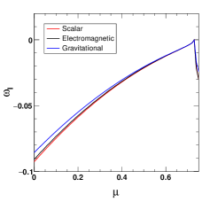
In Fig. 1, we have plotted the real and imaginary quasinormal frequencies w.r.t. GUP parameter with a vanishing cosmological constant i.e. for the black hole defined by the metric (2.27). It is seen that an increase in increases the oscillation frequencies of GWs linearly for all the three perturbations viz., scalar, electromagnetic and gravitational perturbations. The decay rate also increases with increase in . It is seen that for the gravitational perturbation, the quasinormal frequencies and the decay rate are lowest while for the scalar perturbation, they are maximum. An increase in the second GUP parameter , on the other hand, decreases the oscillation frequencies and the decay rate of GWs (see Fig. 2). Thus the effects of these two parameters on the quasinormal modes are opposite.
From Fig. 3, it is seen that the Lorentz symmetry breaking imposes different type of changes on the real part of quasinormal modes depending on the type of perturbation for the black hole (2.27). For the scalar perturbation, with increase in , the real quasinormal frequency decreases. On the hand, in the cases of gravitational perturbation and electromagnetic perturbation, the real quasinormal frequency increases very slowly with increase in . The decay rate of oscillations decrease with increase in the parameter for all the three perturbations. So presence of Lorentz symmetry breaking allows the quasinormal frequencies to propagate further by decreasing the decay rate. The global monopole term shows a different behaviour on the quasinormal modes (see Fig. 4). With increase in , quasinormal frequencies decrease for all the three perturbations and they finally merge when approaches . Similar observation is made for the decay rate of the oscillations also. The decay rate decreases and approaches to zero for all the three perturbation cases. Note that these observations are done for the black hole metric (2.27).
In Fig. 5, we have plotted the real and imaginary quasinormal frequencies for the GUP corrected de Sitter black hole with global monopole with respect to the GUP parameter . In this case we have considered the values of effective cosmological constant allowed by the constraint range provided by the equation (3.12). It is observed that in case of the de Sitter black hole, the quasinormal frequencies for scalar and electromagnetic perturbations are close to each other. The real quasinormal frequencies as well as the imaginary parts increase with increase in the GUP parameter . However in comparison to the case for black hole (2.27), we observe more variation of the quasinormal frequencies with respect to . In case of the decay rate or the imaginary quasinormal modes, we see that for , the decay rates for all the perturbations are almost equal and with increase in , the decay rates changes differently resulting maximum decay rate for the case of scalar perturbations and minimum for the case of gravitational perturbations. On the other hand, in Fig. 6 for the de Sitter black hole, both real and imaginary quasinormal frequencies show a different variation pattern with respect to in comparison with Fig. 2. The real quasinormal frequencies for both scalar and electromagnetic perturbation are very close to each other. The decay rates differ very slightly for all the three perturbations and they decrease and tend to merge with an increase in the parameter . The Lorentz violation also imposes a different variation pattern on the quasinormal frequencies in case of de Sitter black hole. In Fig. 7, one can see that the real quasinormal frequencies for both scalar and electromagnetic perturbations approach each other with an increase in the parameter and towards the higher values of , they are almost indistinguishable. However, the real quasinormal frequencies for the case of gravitational perturbation are smaller and follows a similar trend. The decay rate for all the three perturbations, in case of the de Sitter black hole, decreases with increase in the Lorentz violation and becomes almost indistinguishable in higher values of . From Fig. 8, it is found that the variation of real and imaginary quasinormal frequencies for scalar, electromagnetic and gravitational perturbations with respect to also follow a similar trend but in both graphs, beyond , the results for all the perturbations are identical and show a different behaviour.
In case of the anti-de Sitter black hole, from Fig.s 9, 10 and 11 one can see that the variation trend is similar to the previous cases for the black hole (2.27), but the differences of the quasinormal modes obtained from different perturbations are comparatively large. However, variation of quasinormal modes with respect to the parameter shows that the oscillation frequencies and decay rates for different perturbations may become identical or very close at higher values of as seen from Fig. 12.
Finally, the effect of effective cosmological constant on the quasinormal modes is shown in Fig 13. It is seen that in the de Sitter regime, with increase in the effective de Sitter curvature, real quasinormal frequencies for scalar, electromagnetic and axial gravitational perturbations decrease and approach towards as and beyond this, quasinormal frequencies start to increase again slowly. Similarly, the decay rate decreases for all the three perturbations upto and beyond this, decay rate increases drastically. Important point to note here is that upto , the decay rates for all the three perturbations are very close to each other while, beyond this point the axial gravitational perturbation shows a smaller decay rate and the scalar and electromagnetic perturbations show identical decay rates of oscillations. On the other hand, for the anti-de Sitter background curvature, the real quasinormal modes are distinguishable and they decrease gradually with increase in the value of towards . In this regime, the decay rate decreases towards It is noticed that the decay rate for the electromagnetic perturbation is comparatively higher and scalar perturbation gives smaller decay rate for smaller values of However, when approaches , decay rate for scalar perturbation becomes maximum and for gravitational perturbation becomes minimum. So, it is seen that the decay rates as well as the quasinormal frequencies are highly dependent and could be useful to comment on the nature of once we have sufficient astrophysical observational data on quasinormal modes.
This study shows that the GUP signatures may be found from the quasinormal modes for de Sitter, anti-de Sitter or asymptotically flat black holes. However, in case of de Sitter black holes, it may be difficult to distinguish the quasinormal modes from the scalar perturbation and electromagnetic perturbation. Similarly, we see that Lorentz violation and hence the signatures of QG may be obtained from the quasinormal modes for all the three types of black holes. But, in this case also for the de Sitter black holes, it might be difficult to distinguish between scalar and electromagnetic quasinormal modes. On the other hand, it is found that the presence of global monopoles might make it difficult to distinguish among scalar, electromagnetic and gravitational quasinormal modes for both the de Sitter and anti-de Sitter black holes.
For a clear picture, we compare our results with some previous results in Table 4. The quasinormal modes in GUP corrected Schwarzschild black holes in GR have been studied in Ref. [34] for scalar perturbation. The quasinormal modes in bumblebee gravity have been studied for the first time in Ref. [25]. However, in this study, no other ingredients apart from Lorentz violation have been used. We list some values of quasinormal modes from these two studies in Table 4 along with the corresponding quasinormal modes for the black hole defined by equation (2.27). We see that the percentage deviation of quasinormal modes for this new black hole from the GUP corrected black hole in GR is maximum in the Table 4 for and . With an increase in , we notice a decrease in the deviation of quasinormal modes. An increase in may tend to nullify the effect of Lorentz violation as we have seen previously. Again, we see significant deviations of quasinormal modes from that of the general black hole in bumblebee gravity and it clearly shows the impacts of the GUP parameters and global monopoles. We have also listed the deviations of quasinormal modes from those in GR which show that the quasinormal modes deviate significantly in this new black hole solution with three ingredients viz., Lorentz violation, global monopole and GUP. Once we obtain significant experimental results in the near future, our study might help to differentiate such black hole solutions from those in GR. In other words, the study might help to have some experimental signatures on quasinormal modes for Lorentz violation, global monopole and GUP.
| WKB | Padé averaged WKB | |||
| Time domain | ||||
| WKB | Padé averaged WKB | |||
| Time domain | ||||
| WKB | Padé averaged WKB | |||
| Time domain | ||||
| GUPBH | BBH | Black hole (2.27) | ||||
|---|---|---|---|---|---|---|
5 Evolution of Scalar, Electromagnetic and Gravitational Perturbations on the Black hole geometries
In this section, we study the evolution of the scalar, electromagnetic and gravitational perturbations using the time domain integration method described in Ref. [69]. Defining , , we can express equation (4.3) in the following form:
| (5.1) |
Now, using initial conditions and (here and are median and width of the initial wave-packet), time evolution of the scalar field can be expressed as
| (5.2) |
Here during the numerical procedure we have kept in order to satisfy the Von Neumann stability condition. Using the same procedure for electromagnetic perturbation and gravitational perturbation we have calculated the corresponding time profiles.


In Fig. 14, in the plot on the left, we have shown the time profiles for scalar, electromagnetic and gravitational perturbations for and . It is seen that the oscillation frequency of gravitational perturbation is lower than the other two perturbations supporting the previously obtained results. In the plot on the right, we have shown the dependency of multipole moment on the quasinormal modes for scalar perturbation. The real quasinormal frequencies increase with increase in the multipole moment . However, the multipole moment has a very small impact on the decay rate of the oscillations. These results agree well with the Table 1 where we have calculated the quasinormal modes using Padé averaged th order WKB approximation method. Further, we have used the time domain profiles to calculate the quasinormal modes using the Levenberg Marquardt algorithm [70, 71, 72]. In Fig. 15, we have shown the estimation of quasinormal modes by fitting the time domain profile with and for the scalar perturbation. In Tables 1, 2 and 3, we have shown the quasinormal modes obtained from the time domain analysis along with those obtained from 6th order WKB and 6th order Padé averaged WKB methods. We see that the quasinormal frequencies obtained from the time domain analysis show a good agreement with those obtained from the WKB approximation method.
6 Detection Possibilities of Quasinormal modes
In this section we discuss the possibility of detection of quasinormal modes from such black holes in brief. Following Ref. [73], we assume the mass of the black hole , where is a positive constant, and is equal to , or , or depending upon the value of the cosmological constant. In physical units, the quasinormal frequency and the decay time are expressed as [73]:
| (6.1) | ||||
| (6.2) |
and
| (6.3) | ||||
| (6.4) |
These expressions can allow us to check the possibility of detection of GW signals coming from an perturbed black hole by GW detectors provided we know the sensitive frequency range of the detectors. For the ground based interferometers, like LIGO-Virgo GW detectors the sensitive frequency range is . Using this range for the quasinormal modes from Tables 1, 2 and 3 for calculated using Padé averaged WKB method, we have for the scalar perturbation,
| (6.5) |
for the electromagnetic perturbation,
| (6.6) |
and for the gravitational perturbation,
| (6.7) |
Again, the LISA sensitivity range is from mHz to Hz [74]. So, in case of LISA, for the scalar perturbation
| (6.8) |
for the electromagnetic perturbation,
| (6.9) |
and finally for the gravitational perturbation,
| (6.10) |
If we consider the quasinormal modes from the oscillations of the black hole at the center of our Galaxy i.e. Sagittarius , [75]. It suggests that for all the three perturbations i.e. scalar, electromagnetic and gravitational perturbations, LIGO-Virgo can’t detect the quasinormal frequencies from Sagittarius . However, we see that the quasinormal frequencies from Sagittarius fall within the detection range of LISA. Hence, in the near future it might be possible to comment on the Lorentz violation, global monopole and GUP parameters, and would be possible constrain them using the quasinormal modes from a black hole.
7 Sparsity of Hawking emission
For a black hole at temperature emitting Hawking radiation with frequency in the momentum interval , the energy emitted per unit time or the total power of Hawking radiation is given by [76, 77]
| (7.1) |
where is the unit vector normal to the surface element and is the greybody factor. For massless particles and hence the total power of Hawking radiation can be rewritten as
| (7.2) |
where
| (7.3) |
is the power emitted per unit frequency in the mode. Here the area is a multiple of the horizon area. Although for Schwarzschild black hole, is taken to be times the horizon area, we shall consider i.e. the black hole event horizon area as this consideration will not impact the qualitative result of the study [76].
The excitation of massless uncharged scalar fields around the bumblebee black hole is governed by the Klein-Gordon equation defined in equation (4.3). A portion of the radiation being emitted from the black hole is reflected back by the effective potential of the perturbation while the remaining portion is transmitted out. The greybody factor gives a measurement to the transmission probability of the outgoing Hawking quanta to reach the infinity without being back-scattered by this effective potential.
7.1 Bounds on the greybody factor
Although there are many methods to obtain the greybody factor of a black hole, in this work we follow Refs. [78, 79, 80, 81, 82] to obtain the greybody factor of the black hole defined by the metric (2.27). The general bound on the greybody factor [78] is given by
| (7.4) |
where
| (7.5) |
The arbitrary function has to be positive definite everywhere and satisfy the boundary condition, for the bound (7.4) to hold. However, as a particularly simple choice of , we consider for the present case that
| (7.6) |
Substituting equation (7.6) in equation (7.5) and using the definition of , we get
| (7.7) |
Equation (7.4) in conjunction with equations (4.7), (4.18) (4.23) and (7.7) yields relatively simple expressions for the lower bound of the greybody factor as
| (7.8) |
| (7.9) |
| (7.10) |
where , and denote the greybody factors for the scalar perturbation, electromagnetic perturbation and gravitational perturbation respectively. The expressions show that the GUP correction factors and impact the greybody factor of a black hole along with the Lorentz violation term and the global monopole term . It should be noted that these expressions are derived for the vanishing effective cosmological constant only. To have a better qualitative idea we have plotted the greybody factors for different sets of parameters of the black hole. In Fig. 16, we have plotted the greybody factors with respect to frequency for different values of the first GUP parameter for the scalar, electromagnetic and gravitational perturbations. It is seen that in case of scalar perturbations, the greybody factors decrease comparatively rapidly with the increasing value of than the other two cases. Thus, for all the three perturbations, we have a clear conclusion that an increase in the first GUP parameter , decreases the greybody factor of the black hole. It implies that an increase in decreases the probability of Hawking radiation to reach the spatial infinity. On the other hand, the increase in the second GUP parameter increases the greybody factor of the black hole in case of all the three perturbations (see Fig. 17). However, in both cases, the greybody factor for the gravitational perturbation has less dependency on the parameters and than the other two perturbations. That is GUP correction has less impact on the gravitational perturbation in this respect. Similarly, the dependencies of the greybody factors on the parameters and for the all three perturbations are shown in Fig. 18 and Fig. 19 respectively. We see that the pattern of dependency on is similar to the dependency on the parameter , whereas the dependency on is similar to the case of . However, the impacts of and are highest for the cases of electromagnetic perturbation and scalar perturbation respectively. Among all four parameters, the parameter , i.e. the global monopole seems to have the dominant influence on the greybody factors of all perturbations. Moreover, in all cases the greybody factor for the gravitational perturbation approaches very quickly towards its peak value with respect to the frequency in comparison to the other two perturbations and hence the probability of the hawking radiation to reach the spatial infinity is high in this perturbation.


Using equations (7.8), (7.9) and (7.10) in equation (7.2), one can obtain the total power spectra of the black hole for scalar, electromagnetic and gravitational perturbations respectively. With the help of the black hole power spectra, it is possible to have a quantitative idea on the sparsity of the black hole, which is discussed in the following subsection.
7.2 Sparsity of the Hawking radiation
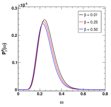
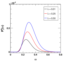
The distribution with respect to frequency provides the necessary insights to study the sparsity of the black hole. In Fig. 20, we have shown the Hawking radiation power spectrum of the black hole for different values of GUP parameter . It is observed that with increase in the parameter value, the peak of the distribution shifts towards the higher frequency and the total Hawking radiation emitted is increased for all the three cases of perturbation. However, it is observed that for the gravitational perturbation, total Hawking radiation emitted is higher. But, for the other GUP parameter , we observe an opposite scenario (see Fig. 21). The Lorentz violation can also increase the total Hawking radiation emitted. From Fig. 22, it is seen that an increase in the parameter increases the total emission and the peak of the distribution shifts towards the higher frequency range. However, the shift is very small in case of the gravitational perturbation. Finally, we consider the variation of the power spectrum for different values of the monopole term and see that an increase in the parameter decreases the total radiation emitted and shifts the peak of the distribution towards the lower frequency ranges. One can see that the changes are significant for the gravitational perturbations also. From the previous results it is seen that in this case, the parameter has a higher influence over the power spectrum of the black hole.


To have a better idea on the radiation emitted by the black holes, we consider the sparsity of the black holes which will give a dimensionless quantitative measure of the Hawking radiation from these black holes. So, for a quantitative idea on the sparsity of Hawking radiation, we define a dimensionless parameter [77, 83, 84, 76, 82] as
| (7.11) |
The parameter in the above expression is the average time interval between the emission of two successive Hawking radiation quanta, defined as
| (7.12) |
where is the frequency corresponding to the peak of the black hole power spectrum, which can be easily determined from the power spectrum distribution curves we have studied. is the characteristic time for the emission of individual Hawking quantum, defined by
| (7.13) |
where , the localisation time-scale is the characteristic time taken by the emitted wave field with frequency to complete one cycle of oscillation. So, clearly implies extremely sparse Hawking cascade i.e. the time interval between successive Hawking quanta emission is much larger than the time required for the emission of individual Hawking quantum and suggests that the Hawking radiation flow is almost continuous.
| Scalar perturbation | Electromagnetic perturbation | |||||
| Gravitational perturbation | ||||||
| Scalar perturbation | Electromagnetic perturbation | |||||
| Gravitational perturbation | ||||||
| Scalar perturbation | Electromagnetic perturbation | |||||
| Gravitational perturbation | ||||||
| Scalar perturbation | Electromagnetic perturbation | |||||
| Gravitational perturbation | ||||||
Now, to have a quantitative idea, we have shown the calculated sparsity of the black holes in Tables 5, 6, 7 and 8 for different black hole parameters and perturbations. In Table 5, we have shown the i.e. the frequency corresponding to the peak in the power spectrum and the sparsity for scalar, electromagnetic and gravitational perturbations for different values of the Lorentz violation parameter . We see that with increase in the parameter , the sparsity decreases for all the three perturbations. In case of the scalar perturbations, the sparsity of the black hole is very high and in case of the gravitational perturbations, sparsity is less. This shows that in case of gravitational perturbations, the Hawking radiation is less sparse and the time between the emission of two successive Hawking quanta is comparatively less than that for the electromagnetic perturbations and scalar perturbations. The results also show that the variations are not very small and hence the Hawking radiation may be a useful way to obtain the signature of Lorentz violating and the possibility of quantum gravity in the near future.
In case of the GUP parameters (see Tables 6 and 7), although the variations are monotonic and stable, they are very small and practically not possible to obtain the signatures of GUP corrections from the sparsity of the black holes. While in case of Table 8, where we have considered the variations of sparsity of the black hole with the parameter , it is seen that an increase in the value of increases the sparsity of the Hawking radiation cascade of the black hole drastically. The variations are more distinctive in case of the scalar perturbations and less distinctive in case of gravitational perturbations. These results show that the existence of a global monopole has a significant impacts over the sparsity of the black holes and a higher value of might make the black holes very sparse. This will increase the time gap between the two successive Hawking radiation quanta.
7.3 Area Spectrum from Adiabatic Invariance
Finally, following Refs. [85, 86] we derive the area spectrum of the black hole which is useful for the further study of sparsity of the black hole. We apply the Wick rotation in the Lorentzian time and thus transforming time to , we write the Euclideanized form of the metric in the following way:
| (7.14) |
where , and means the Euclidean time. Considering the only dynamic freedom of adiabatic invariants to be the radial coordinate , the adiabatic invariant can be simply expressed [87] as
| (7.15) |
where is the conjugate momentum to the coordinate . Now, considering only the outgoing path and ignoring whether the particle has mass or not [88], from Hamilton’s canonical equation,
| (7.16) |
where and , is the mass of the black hole from which a particle with energy tunnels through its horizon. Using equation (7.16) into equation (7.15), we may write
| (7.17) |
This equation (7.17) can be further written as
| (7.18) |
where we have used the assumption that the particles moving in the black hole background spacetime have the same periodicity as the background spacetime [89]. At last, using the definitions of the black hole mentioned above, we found that
| (7.19) |
From the Bohr-Sommerfeld quantization rule, , , so the quantized area of the black hole is now given by
| (7.20) |
Hence the area spectrum of the black hole is different from that of Schwarzschild one by a multiplicative factor of and is given by
| (7.21) |
The equations (7.3) with the above equation (7.21) show that the power spectrum of the black hole is also quantized and is differed from the quantization rule of Schwarzschild black hole by a factor of . Hence, it is seen that the Lorentz violation can have impacts over the area spectrum of the black hole and consequently on the Hawking radiation emitted by the black hole.
8 Conclusion
In this work, we have used three elements viz., bumblebee field, global monopole and GUP corrections to study the properties of the black hole in this configuration. We have previously mentioned that the bumblebee field can effectively result in Lorentz violation and in Lorentz violating theories topological defects like global monopoles may arise. Being isolated, global monopoles may be present in the universe till now and can influence the black hole properties including quasinormal modes as we have seen. The GUP corrections provide the quantum effects to the black hole and previous studies suggest that they are connected with Lorentz violation [54, 55]. Hence, inclusion of all these three ingredients may provide a realistic platform to study the properties of the black hole. It should be noted that such a configuration with all three ideas has not been studied before. So we believe this study will contribute significantly in the studies of the impacts by Lorentz violation, GUP and global monopole on the quasinormal modes.
This study shows that the GUP correction can affect the quasinormal modes of the black holes. An increase in the GUP parameter increases the quasinormal frequencies and the decay rates. While the other GUP parameter has an opposite impact on the quasinormal modes. It is seen that the impacts of the GUP parameters are more significant in the de Sitter black hole and less significant in the anti-de Sitter black hole.
The Lorentz violation also affects the quasinormal modes. We observe that for and for anti-de Sitter case, the scalar quasinormal frequency decreases with an increase in the violation parameter value but the electromagnetic and gravitational quasinormal modes increase with an increase in the value of the violation parameter. However, for the de Sitter black hole, quasinormal frequencies decrease for all the perturbation schemes considered in this work. The decay rate in all three cases of perturbations decreases with increase in violation parameter. On the other hand, an increase in the global monopole parameter results in decrease of the quasinormal frequency as well as the decay rate. The impact of the monopole term on quasinormal modes is higher in comparison to the GUP parameters and in de Sitter regime, the impact pattern of the second GUP deformation parameter resembles with it for small values of the parameters.
The quasinormal modes in the de Sitter regime are quite different from those we have obtained for anti-de Sitter and vanishing cosmological constant cases. This variation can be definitely useful in inferring a bound on the cosmological constant provided we have significant experimental results from the next generation gravitational wave detectors in the near future. One may note that there is a theoretical constraint on the de Sitter spacetime given by equation (3.12) which is controlled by the global monopole and the Lorentz violation term. For a viable de Sitter solutions, global monopole term should be less than and the Lorentz violation term should be greater than . An increase in both the parameters by respecting these limits reduces the ranges of viable de Sitter solutions. So, experimental constraints on global monopoles and the Lorentz violation parameter could be helpful in introducing bounds on the cosmological constant.
Moreover, we see that this study might help to differentiate the impacts of GUP and global monopoles on the black hole. Although GUP and global monopole impacts may be apparently indistinguishable for very small values of the parameters, for comparatively large values we can see a clear difference in the quasinormal modes. So, in general, the quasinormal modes have a higher dependency on global monopoles than GUP. This property may be helpful to check the existence of a global monopoles on the black hole spacetime once we have a significant experimental result from LISA in the near future.
It is worth to be mentioned that the GUP impacts on quasinormal modes of a Schwarzschild black hole have been studied previously [34]. However, in this study, we have considered three perturbations viz., scalar, electromagnetic and gravitational perturbations and compared the results in presence of bumblebee field, global monopole and cosmological constant. It clearly shows that the GUP impacts highly depend on the Lorentz violation, cosmological constant and presence of global monopoles. As we have mentioned in the introduction, quasinormal modes and greybody factors have been extensively studied in different modified theories of gravity including Rastall gravity, gravity etc. We have seen that for different model parameters in different modified gravity theories, the quasinormal modes may show a different variation pattern. For example, in a recent study the authors studied the impacts of energy momentum conservation violating Rastall parameter on the quasinormal modes [26]. It is seen that the impacts of general energy momentum conservation violation on quasinormal modes differ from that of Lorentz violation. We believe that such studies might be helpful to differentiate between different theories and bumblebee gravity in terms of quasinormal modes in the near future.
In the next part of study, we have studied the quantum thermodynamics of the black holes. Here at first we have obtained the Hawking temperature of the black holes within the framework of GUP for scalar, electromagnetic and gravitational perturbations. Then we have obtained the greybody factors of the black holes. We see that the Lorentz violation affects the greybody factor and greybody factor decreases with an increase in the parameter value. Low values of greybody factor imply a low probability of the Hawking radiation to reach spatial infinity. So, future astrophysical observations may shed more light in this area and may provide support to the indirect evidence of Lorentz violation. On the other hand, the topological defects have an opposite impact on the greybody factors. We see that an increase in decreases the greybody factors and increases the probability of Hawking radiation to reach the spatial infinity. The GUP parameter also provides a similar effect on the greybody factors; however the effect is less in comparison to the previous case. An increase in the GUP parameter , on the other hand, decreases the probability of Hawking radiation to reach spatial infinity. So the study shows that the parameters and have a similar impact on the greybody factors.
Total Hawking radiation power emitted increases with an increase in GUP parameter and Lorentz violation parameter . On the contrary, it decreases with increase the second GUP parameter and global monopole term and the peak of the distribution shifts towards low frequency range.
In the case of gravitational perturbation, the black hole is less sparse and in the case of scalar perturbation the black hole is highly sparse. In the case of all the three perturbations, with an increase in the Lorentz violation factor, the sparsity of the black holes decreases. On the other hand, the GUP parameters have a very very small impact on the sparsity of the black holes. With increase in the global monopole term, , the sparsity of the black hole increases.
The global monopole parameter does not imprint significant changes on the black hole sparsity in case of gravitational perturbation. Since the peak of the power spectrum for the gravitational perturbation is much higher and is at near the low frequency range, it results in the Hawking radiation to be less sparse in comparison to the scalar and electromagnetic perturbations. Also due to this high value of power spectrum peak, the impacts of the black hole parameters including global monopole on the gravitational perturbation is not as large as we have observed for the other two perturbations, i.e. electromagnetic and scalar perturbations. This should be a universal feature of the sparsity of black holes as the gravitational perturbation around any black hole should be of a similar nature except some local effects introduced by the black hole type-parameters and its background. However, the effects due to the black hole background and the model parameters should be small like our case and hence such small variations represent the unique structure of a black hole solution.
Eventually, we have checked the area quantization of the black hole by using the adiabatic invariance method. It shows that the area quantization is affected by the presence of Lorentz violation. Therefore, we can conclude that the Hawking radiation power emitted is also quantized and the quantization is affected by the Lorentz violation. Recent studies show the impacts of area quantization of black holes on GW echoes [44, 45, 46]. So, it can be possible in the near future to comment on the fate of quantum gravity and Lorentz violation provided we have sufficient astrophysical signatures.
References
- [1] V. A. Kostelecký, Lorentz violation, and the standard model, Phys. Rev. D 69, 105009 (2004) [arXiv:hep-th/0312310].
- [2] R. Casana, A. Cavalcante, F. P. Poulis, and E. B. Santos, Exact Schwarzschild-like Solution in a Bumblebee Gravity Model, Phys. Rev. D 97, 104001 (2018) [arXiv:1711.02273].
- [3] R. Bluhm and V. A. Kostelecký, Spontaneous Lorentz Violation, Nambu-Goldstone Modes, and Gravity, Phys. Rev. D 71, 065008 (2005) [arXiv:hep-th/0412320].
- [4] Q. G. Bailey and V. A. Kostelecký, Signals for Lorentz Violation in Post-Newtonian Gravity, Phys. Rev. D 74, 045001 (2006) [arXiv:gr-qc/0603030].
- [5] Q. G. Bailey, Time Delay and Doppler Tests of the Lorentz Symmetry of Gravity, Phys. Rev. D 80, 044004 (2009) [arXiv:0904.0278].
- [6] R. Tso and Q. G. Bailey, Light-Bending Tests of Lorentz Invariance, Phys. Rev. D 84, 085025 (2011) [arXiv:1108.2071].
- [7] V. A. Kostelecký and J. D. Tasson, Prospects for Large Relativity Violations in Matter-Gravity Couplings, Phys. Rev. Lett. 102, 010402 (2009) [arXiv:0810.1459].
- [8] R. V. Maluf, V. Santos, W. T. Cruz, and C. A. S. Almeida, Matter-Gravity Scattering in the Presence of Spontaneous Lorentz Violation, Phys. Rev. D 88, 025005 (2013) [arXiv:1304.2090].
- [9] R. V. Maluf, C. A. S. Almeida, R. Casana, and M. M. Ferreira, Einstein-Hilbert Graviton Modes Modified by the Lorentz-Violating Bumblebee Field, Phys. Rev. D 90, 025007 (2014) [arXiv:1402.3554].
- [10] A. F. Santos, W. D. R. Jesus, J. R. Nascimento, and A. Yu. Petrov, Gödel Solution in the Bumblebee Gravity, Mod. Phys. Lett. A 30, 1550011 (2015) [arXiv:1407.5985].
- [11] V. A. Kostelecký, A. C. Melissinos, and M. Mewes, Searching for Photon-Sector Lorentz Violation Using Gravitational-Wave Detectors, Phys. Lett. B 761, 1 (2016) [arXiv:1608.02592].
- [12] V. A. Kostelecký and M. Mewes, Testing Local Lorentz Invariance with Gravitational Waves, Phys. Lett. B 757, 510 (2016) [arXiv:1602.04782].
- [13] S. Kumar Jha, H. Barman, and A. Rahaman, Bumblebee Gravity and Particle Motion in Snyder Noncommutative Spacetime Structures, J. Cosmol. Astropart. Phys. 04, 036 (2021) [arXiv:2012.02642].
- [14] S. Kanzi and İ. Sakallı, GUP Modified Hawking Radiation in Bumblebee Gravity, Nuclear Physics B 946, 114703 (2019).
- [15] S. K. Jha, S. Aziz, and A. Rahaman, Study of Einstein-Bumblebee Gravity with Kerr-Sen-like Solution in the Presence of a Dispersive Medium, Eur. Phys. J. C 82, 106 (2022) [arXiv:2103.17021].
- [16] İ. Güllü and A. Övgün, Schwarzschild-like Black Hole with a Topological Defect in Bumblebee Gravity, Annals of Physics 436, 168721 (2022).
- [17] A. Övgün, K. Jusufi, and İ Sakallı, Exact Traversable Wormhole Solution in Bumblebee Gravity, Phys. Rev. D 99, 024042 (2019) [arXiv:1804.09911 [gr-qc]].
- [18] C. V. Vishveshwara, Stability of the Schwarzschild Metric, Phys. Rev. D 1, 2870 (1970).
- [19] W. H. Press, Long Wave Trains of Gravitational Waves from a Vibrating Black Hole, ApJ 170, L105 (1971).
- [20] S. Chandrasekhar and S. Detweiler, The Quasi-Normal Modes of the Schwarzschild Black Hole, Proc. R. Soc. Lond. A 344, 441 (1975).
- [21] C. Ma, Y. Gui, W. Wang, F. Wang, Massive scalar field quasinormal modes of a Schwarzschild black hole surrounded by quintessence, Cent. Eur. J. Phys. 6, 194 (2008) [arXiv:gr-qc/0611146].
- [22] D. J. Gogoi and U. D. Goswami, A New f(R) Gravity Model and Properties of Gravitational Waves in It, Eur. Phys. J. C 80, 1101 (2020) [arXiv:2006.04011].
- [23] D. J. Gogoi and U. D. Goswami, Gravitational Waves in Gravity Power Law Model, Indian J. Phys. 96, 637 (2022) [arXiv:1901.11277].
- [24] D. Liang, Y. Gong, S. Hou and Y. Liu, Polarizations of Gravitational Waves in Gravity, Phys. Rev. D 95, 104034 (2017) [arXiv:1701.05998].
- [25] R. Oliveira, D. M. Dantas, and C. A. S. Almeida, Quasinormal Frequencies for a Black Hole in a Bumblebee Gravity, EPL 135, 10003 (2021) [arXiv:2105.07956].
- [26] D. J. Gogoi and U. D. Goswami, Quasinormal Modes of Black Holes with Non-Linear-Electrodynamic Sources in Rastall Gravity, Physics of the Dark Universe 33, 100860 (2021) [arXiv:2104.13115].
- [27] J. P. M. Graça and I. P. Lobo, Scalar QNMs for Higher Dimensional Black Holes Surrounded by Quintessence in Rastall Gravity, Eur. Phys. J. C 78, 101 (2018) [arXiv:1711.08714].
- [28] Y. Zhang, Y.X. Gui, F. Li, Quasinormal modes of a Schwarzschild black hole surrounded by quintessence: electromagnetic perturbations, Gen. Relativ. Gravit. 39, 1003 (2007) [arXiv:gr-qc/0612010].
- [29] M. Bouhmadi-López, S. Brahma, C.-Y. Chen, P. Chen, and D. Yeom, A Consistent Model of Non-Singular Schwarzschild Black Hole in Loop Quantum Gravity and Its Quasinormal Modes, J. Cosmol. Astropart. Phys. 07, 066 (2020) [arXiv:2004.13061].
- [30] J. Liang, Quasinormal Modes of the Schwarzschild Black Hole Surrounded by the Quintessence Field in Rastall Gravity, Commun. Theor. Phys. 70, 695 (2018).
- [31] Y. Hu, C.-Y. Shao, Y.-J. Tan, C.-G. Shao, K. Lin, and W.-L. Qian, Scalar Quasinormal Modes of Nonlinear Charged Black Holes in Rastall Gravity, EPL 128, 50006 (2020).
- [32] S. Giri, H. Nandan, L. K. Joshi, and S. D. Maharaj, Geodesic Stability and Quasinormal Modes of Non-Commutative Schwarzschild Black Hole Employing Lyapunov Exponent, Eur. Phys. J. Plus 137, 181 (2022).
- [33] D. J. Gogoi, R. Karmakar, and U. D. Goswami, Quasinormal Modes of Non-Linearly Charged Black Holes Surrounded by a Cloud of Strings in Rastall Gravity, arXiv:2111.00854 (2021).
- [34] M. A. Anacleto, J. A. V. Campos, F. A. Brito, and E. Passos, Quasinormal Modes and Shadow of a Schwarzschild Black Hole with GUP, Annals of Physics 434, 168662 (2021) [arXiv:2108.04998].
- [35] R. G. Daghigh and M. D. Green, Validity of the WKB Approximation in Calculating the Asymptotic Quasinormal Modes of Black Holes, Phys. Rev. D 85, 127501 (2012) [arXiv:1112.5397 [gr-qc]].
- [36] P. Boonserm, T. Ngampitipan, and P. Wongjun, Greybody Factor for Black Holes in DRGT Massive Gravity, Eur. Phys. J. C 78, 492 (2018) [arXiv:1705.03278 [gr-qc]].
- [37] M. Okyay and A. Övgün, Nonlinear Electrodynamics Effects on the Black Hole Shadow, Deflection Angle, Quasinormal Modes and Greybody Factors, J. Cosmol. Astropart. Phys. 2022, 009 (2022) [arXiv:2108.07766 [gr-qc]].
- [38] P. Boonserm, T. Ngampitipan, and P. Wongjun, Greybody Factor for Black String in DRGT Massive Gravity, Eur. Phys. J. C 79, 330 (2019) [arXiv:1902.05215 [gr-qc]].
- [39] W. Javed, I. Hussain, and A. Övgün, Weak Deflection Angle of Kazakov-Solodukhin Black Hole in Plasma Medium Using Gauss-Bonnet Theorem and Its Greybody Bonding, Eur. Phys. J. Plus 137, 148 (2022) [arXiv:2201.09879 [gr-qc]].
- [40] A. Övgün and K. Jusufi, Quasinormal Modes and Greybody Factors of Gravity Minimally Coupled to a Cloud of Strings in Dimensions, Annals of Physics 395, 138 (2018) [arXiv:1801.02555 [gr-qc]].
- [41] R. G. Daghigh, M. D. Green, J. C. Morey, and G. Kunstatter, Scalar Perturbations of a Single-Horizon Regular Black Hole, Phys. Rev. D 102, 104040 (2020) [arXiv:2009.02367 [gr-qc]].
- [42] A. Övgün and K. Jusufi, Massive Vector Particles Tunneling From Noncommutative Charged Black Holes and Its GUP-Corrected Thermodynamics, Eur. Phys. J. Plus 131, 177 (2016) [arXiv:1512.05268 [gr-qc]].
- [43] A. Övgün and K. Jusufi, The Effect of GUP to Massive Vector and Scalar Particles Tunneling From a Warped DGP Gravity Black Hole, Eur. Phys. J. Plus 132, 298 (2017) [arXiv:1703.08073].
- [44] V. Cardoso, V. F. Foit, and M. Kleban, Gravitational Wave Echoes from Black Hole Area Quantization, J. Cosmol. Astropart. Phys. 08, 006 (2019) [arXiv:1902.10164].
- [45] S. Datta and K. S. Phukon, Imprint of Black Hole Area Quantization and Hawking Radiation on Inspiraling Binary, Phys. Rev. D 104, 124062 (2021) [arXiv:2105.11140].
- [46] A. Coates, S. H. Völkel, and K. D. Kokkotas, On Black Hole Area Quantization and Echoes, Class. Quantum Grav. 39, 045007 (2022) [arXiv:2201.03245].
- [47] V. A. Kostelecký and N. Russell, Data Tables for Lorentz and C P T Violation, Rev. Mod. Phys. 83, 11 (2011).
- [48] M. D. Seifert, Monopole Solution in a Lorentz-Violating Field Theory, Phys. Rev. Lett. 105, 201601 (2010).
- [49] V. A. Kostelecký and S. Samuel, Gravitational Phenomenology in Higher-Dimensional Theories and Strings, Phys. Rev. D 40, 1886 (1989).
- [50] S. M. Carroll, J. A. Harvey, V. A. Kostelecký, C. D. Lane, and T. Okamoto, Noncommutative Field Theory and Lorentz Violation, Phys. Rev. Lett. 87, 141601 (2001).
- [51] T. W. B. Kibble, Topology of Cosmic Domains and Strings, J. Phys. A: Math. Gen. 9, 1387 (1976).
- [52] A. H. Guth, Inflationary Universe: A Possible Solution to the Horizon and Flatness Problems, Phys. Rev. D 23, 347 (1981).
- [53] R. Durrer, M. Kunz, and A. Melchiorri, Cosmic Structure Formation with Topological Defects, Physics Reports 364, 1 (2002).
- [54] A. N. Tawfik, H. Magdy, and A. F. Ali, Lorentz Invariance Violation and Generalized Uncertainty Principle, Phys. Part. Nuclei Lett. 13, 59 (2016).
- [55] G. Lambiase and F. Scardigli, Lorentz Violation and Generalized Uncertainty Principle, Phys. Rev. D 97, 075003 (2018).
- [56] O. Bertolami and J. Páramos, Vacuum Solutions of a Gravity Model with Vector-Induced Spontaneous Lorentz Symmetry Breaking, Phys. Rev. D 72, 044001 (2005).
- [57] M. A. Anacleto, F. A. Brito, J. A. V. Campos, and E. Passos, Quantum-Corrected Scattering and Absorption of a Schwarzschild Black Hole with GUP, Phys. Lett. B 810, 135830 (2020) [arXiv:2003.13464].
- [58] S. Gangopadhyay, A. Dutta, and M. Faizal, Constraints on the Generalized Uncertainty Principle from Black-Hole Thermodynamics, EPL 112, 20006 (2015) [arXiv:1501.01482].
- [59] A. F. Ali, S. Das, and E. C. Vagenas, Discreteness of Space from the Generalized Uncertainty Principle, Phys. Lett. B 678, 497 (2009) [arXiv:0906.5396].
- [60] A. N. Tawfik and A. M. Diab, Generalized Uncertainty Principle: Approaches and Applications, Int. J. Mod. Phys. D 23, 1430025 (2014) [arXiv:1410.0206].
- [61] A. N. Tawfik and E. A. El Dahab, Corrections to Entropy and Thermodynamics of Charged Black Hole Using Generalized Uncertainty Principle, Int. J. Mod. Phys. A 30, 1550030 (2015) [arXiv:1501.01286].
- [62] R. V. Maluf and J. C. S. Neves, Black Holes with a Cosmological Constant in Bumblebee Gravity, Phys. Rev. D 103, 044002 (2021) [arXiv:2011.12841].
- [63] S. Chandrasekhar, The mathematical theory of black holes, Oxford University Press, Oxford (1992).
- [64] C.-Y. Chen and P. Chen, Gravitational perturbations of nonsingular black holes in conformal gravity, Phys. Rev. D 99, 104003 (2019) [arXiv:1902.01678].
- [65] B. F. Schutz and C. M. Will, Black Hole Normal Modes - A Semi analytic Approach, The Astrophysical Journal 291, L33 (1985).
- [66] S. Iyer and C. M. Will, Black-Hole Normal Modes: A WKB Approach. I. Foundations and Application of a Higher-Order WKB Analysis of Potential-Barrier Scattering, Phys. Rev. D 35, 3621 (1987).
- [67] R. A. Konoplya, Quasinormal Behavior of the D -Dimensional Schwarzschild Black Hole and the Higher Order WKB Approach, Phys. Rev. D 68, 024018 (2003) [arXiv:gr-qc/0303052].
- [68] J. Matyjasek and M. Telecka, Quasinormal Modes of Black Holes. II. Padé Summation of the Higher-Order WKB Terms, Phys. Rev. D 100, 124006 (2019) [arXiv:1908.09389].
- [69] C. Gundlach, R. H. Price and J. Pullin, Late time behavior of stellar collapse and explosions: 2. Nonlinear evolution, Phys. Rev. D 49, 890 (1994) [arXiv:gr-qc/9307010].
- [70] K. Levenberg, A Method for the Solution of Certain Non-Linear Problems in Least Squares, Quart. Appl. Math. 2, 164 (1944).
- [71] D. W. Marquardt, An Algorithm for Least-Squares Estimation of Nonlinear Parameters, Journal of the Society for Industrial and Applied Mathematics 11, 431 (1963).
- [72] E. Berti, V. Cardoso, J. A. González, and U. Sperhake, Mining Information from Binary Black Hole Mergers: A Comparison of Estimation Methods for Complex Exponentials in Noise, Phys. Rev. D 75, 124017 (2007) [arXiv:gr-qc/0701086].
- [73] V. Ferrari and L. Gualtieri, Quasi-Normal Modes and Gravitational Wave Astronomy, Gen. Relativ. Gravit. 40, 945 (2008).
- [74] K. Yamamoto, C. Vorndamme, O. Hartwig, M. Staab, T. S. Schwarze, and G. Heinzel, Experimental Verification of Intersatellite Clock Synchronization at LISA Performance Levels, Phys. Rev. D 105, 042009 (2022).
- [75] A. M. Ghez, S. Salim, S. D. Hornstein, A. Tanner, J. R. Lu, M. Morris, E. E. Becklin, and G. Duchene, Stellar Orbits around the Galactic Center Black Hole, ApJ 620, 744 (2005).
- [76] Y.-G. Miao and Z.-M. Xu, Hawking Radiation of Five-Dimensional Charged Black Holes with Scalar Fields, Phys. Lett. B 772, 542 (2017).
- [77] F. Gray, S. Schuster, A. Van–Brunt, and M. Visser, The Hawking Cascade from a Black Hole Is Extremely Sparse, Class. Quantum Grav. 33, 115003 (2016).
- [78] M. Visser, Some General Bounds for One-Dimensional Scattering, Phys. Rev. A 59, 427 (1999) [arXiv:quant-ph/9901030].
- [79] P. Boonserm and M. Visser, Bounding the Bogoliubov Coefficients, Annals of Physics 323, 2779 (2008) [arXiv:0801.0610].
- [80] P. Boonserm and M. Visser, Bounding the Greybody Factors for Schwarzschild Black Holes, Phys. Rev. D 78, 101502 (2008) [arXiv:0806.2209].
- [81] P. Boonserm, T. Ngampitipan, and M. Visser, Bounding the Greybody Factors for Scalar Field Excitations on the Kerr-Newman Spacetime, J. High Energ. Phys. 2014, 113 (2014) [arXiv:1401.0568].
- [82] A. Chowdhury and N. Banerjee, Greybody Factor and Sparsity of Hawking Radiation from a Charged Spherical Black Hole with Scalar Hair, Phys. Lett. B 805, 135417 (2020).
- [83] S. Hod, The Hawking Cascades of Gravitons from Higher-Dimensional Schwarzschild Black Holes, Phys. Lett. B 756, 133 (2016) [arXiv:1605.08440].
- [84] S. Hod, The Hawking Evaporation Process of Rapidly-Rotating Black Holes: An Almost Continuous Cascade of Gravitons, Eur. Phys. J. C 75, 329 (2015) [arXiv:1506.05457].
- [85] B. R. Majhi and E. C. Vagenas, Black hole spectroscopy via adiabatic invariance, Phys. Lett. B 701, 623 (2011) [arXiv:1106.2292].
- [86] Q.-Q. Jiang and Y. Han, On black hole spectroscopy via adiabatic invariance, Phys. Lett. B 718, 584 (2012) [arXiv:1210.4002].
- [87] M. Shahjalal, Area and entropy quantization of quantum-corrected Schwarzschild black hole surrounded by quintessence, Int. J. Mod. Phys. A 34, 1950091 (2019).
- [88] K. Umetsu, Hawking radiation from Kerr–Newman black hole and tunneling mechanism, Int. J. Mod. Phys. A 25, 4123 (2010) [arXiv:0907.1420 [hep-th]].
- [89] G. W. Gibbons and M. J. Perry, Black holes and thermal Green functions, Proc. R. Soc. 358, 467 (1978).