Quasi-resonant diffusion of wave packets in one-dimensional disordered mosaic lattices
Abstract
We investigate numerically the time evolution of wave packets incident on one-dimensional semi-infinite lattices with mosaic modulated random on-site potentials, which are characterized by the integer-valued modulation period and the disorder strength . For Gaussian wave packets with the central energy and a small spectral width, we perform extensive numerical calculations of the disorder-averaged time-dependent reflectance, , for various values of , , and . We find that the long-time behavior of obeys a power law of the form in all cases. In the presence of the mosaic modulation, is equal to 2 for almost all values of , implying the onset of the Anderson localization, while at a finite number of discrete values of dependent on , approaches 3/2, implying the onset of the classical diffusion. This phenomenon is independent of the disorder strength and arises in a quasi-resonant manner such that varies rapidly from 3/2 to 2 in a narrow energy range as varies away from the quasi-resonance values. We deduce a simple analytical formula for the quasi-resonance energies and provide an explanation of the delocalization phenomenon based on the interplay between randomness and band structure and the node structure of the wave functions. We explore the nature of the states at the quasi-resonance energies using a finite-size scaling analysis of the average participation ratio and find that the states are neither extended nor exponentially localized, but ciritical states.
I Introduction
Anderson localization of classical waves and quantum particles occurs due to the interference of multiply scattered waves in spatially random media. Since it was discovered theoretically over 60 years ago by Anderson, it has been studied extensively in many areas of physics [1, 2, 3]. Anderson localization arises universally for all kinds of waves and many aspects of the phenomenon have been explored and understood in detail [4, 5, 6, 7]. Nevertheless, there still exist features which are not fully understood and new aspects of localization continue to be discovered when new elements are included in the system [8, 9, 10, 11, 12, 13].
One of the prominent results of early theories of localization is that in the simplest one-dimensional (1D) and two-dimensional random systems, all eigenstates are exponentially localized even in the presence of infinitesimally weak disorder [14]. However, it has been found that this conclusion is not always true in more general random systems and there exist various situations where some states are not exponentially localized, but are either extended or critically localized. Representative examples include the cases where distinct kinds of impedance matching phenomena such as the Brewster anomaly [15, 16, 17, 18, 19, 20] and the Klein effect [21, 22, 23, 24] happen or the random potential is spatially correlated with short- or long-range correlations [25, 26, 27, 28, 29, 30, 31, 32, 33, 34]. For instance, it has been demonstrated both theoretically and experimentally that there exist extended states at two energy values in the 1D random dimer model which contains a special type of short-range correlated disorder [25, 26]. This model has been generalized to the case of random -mer systems and analytical expressions for the values of the resonant energies at which delocalization arises have been obtained [27, 28, 29, 30].
A discrete set of delocalized states can appear in short-range correlated random systems. In contrast, a continuum of delocalized states with sharp mobility edges was predicted theoretically and confirmed experimentally to appear in long-range correlated random systems in 1D [31, 32, 33, 34, 35, 36, 37]. The mobility edges, which are the energy values separating localized and extended states, can also be present in a wide range of quasiperiodic models in 1D [38, 39, 40, 41, 42, 43, 44, 45, 46, 47, 48, 49]. Recently, an exactly solvable 1D model with multiple mobility edges called quasiperiodic mosaic lattice model has been proposed [43]. In that model, a quasiperiodic on-site potential exists only at periodically spaced sites, while the potential is constant at all other sites. The number and the positions of the mobility edges have been shown to depend sensitively on the modulation period .
The main aim of the present paper is to propose a new way of inducing delocalized states in 1D random systems. We consider a random version of the quasiperiodic mosaic lattice model, which we call disordered mosaic lattice model, where the on-site potential takes a random value only at equally spaced sites with a period . We study the transport and localization properties of the proposed model primarily by investigating the time evolution of wave packets incident on an effectively semi-infinite disordered mosaic lattice chain. More specifically, we calculate the time-dependent reflectance averaged over a large number of independent disorder configurations, , for various values of the modulation period and the central energy of the wave packet, . This approach based on the reflection geometry has substantial experimental advantages over those based on the transmission geometry.
We are especially interested in exploring the long-time scaling behavior of , which obeys a power-law decay of the form for all values of the parameters. From many previous researches, it has been solidly established that in the cases where the standard Anderson localization occurs, the exponent is equal to 2, while in those where the classical diffusion occurs, it is 3/2 [50, 51, 52, 53, 54, 55, 56, 57, 58]. From extensive numerical calculations, we will find that in the presence of the mosaic modulation, is equal to 2 for almost all values of , while at a finite number of discrete values of dependent on , approaches 3/2. In other words, although most eigenstates of the disordered mosaic lattice model are exponentially localized, there appear a finite number of discrete states that are not exponentially localized but display transport behavior characteristic of classical diffusion. We will also find that this phenomenon is independent of the disorder strength and occurs in a quasi-resonant manner. From the numerical results, we will deduce a simple analytical formula for the quasi-resonance energies at which delocalization occurs and provide an explanation of the phenomenon based on the interplay between randomness and band structure and the node structure of the wave functions. We also explore the nature of the states at the quasi-resonance energies using a finite-size scaling analysis of the average participation ratio and find that the states are neither extended nor exponentially localized, but ciritical states.
The rest of this paper is organized as follows. In Sec. II, we introduce the 1D disordered mosaic lattice model characterized by the time-independent Schrödinger equation within the nearest-neighbor tight-binding approximation. We also describe the numerical calculation method and the physical quantities of interest. In Sec. III, we present the numerical results and discuss the mechanism for the onset of the diffusive behavior. We also explore the nature of the states at the quasi-resonance energies using a finite-size scaling analysis of the average participation ratio. Finally, in Sec. IV, we conclude the paper.
II Theoretical model and method
II.1 Model
To describe 1D non-interacting spinless particle systems, we use the standard single-chain tight-binding model
| (1) |
where and are the wave function amplitude and the on-site potential at the -th lattice site respectively. is the energy and is the coupling strength between nearest-neighbor sites. From now on, we will measure all energy scales in units of and set it equal to 1. In this study, we will investigate the transport and localization properties of a model which we call disordered mosaic lattice model. This model is defined by
| (4) |
where the inlay parameter representing the period of the mosaic modulation is a fixed positive integer larger than 1 and is an integer running from 1 to . Then the total number of sites is equal to . The on-site potential at the -th site is a random variable uniformly distributed in the interval , where is the strength of disorder. In all other sites, the on-site potential takes a constant value of . In [43], the authors have studied a quasiperiodic mosaic lattice model, where is a quasiperiodic potential of Aubry-André-type [59]. Our model is different from that model in that is random instead of quasiperiodic. We note that if is a constant potential different from , the model becomes perfectly periodic with period .
II.2 Method
Following the procedure given in [58], we first assume that a monochromatic wave of energy is incident from the left side of the disordered region and define the amplitudes of the incident, reflected, and transmitted waves , , and by
| (7) |
where is related to by the free-space dispersion relation . In the absence of dissipation, the law of energy conservation should be satisfied. In order to solve Eq. (1) numerically, we first fix to 1, then we obtain and . Knowing the values of and , we can solve Eq. (1) iteratively to obtain , , , , . Using the definition of and given in Eq. (7), we can express them in terms of and :
| (8) |
We are interested in the case where the length of the disordered region is sufficiently large. Then the large portion of the incident wave power will be reflected. Therefore we focus on the behavior of the reflection coefficient and the reflectance defined by
| (9) |
Next we consider a Gaussian wave packet characterized by the spectrum
| (10) |
where is the central energy of the wave packet and is its spectral width. satisfies
| (11) |
The time-dependent reflection coefficient of the incident Gaussian wave packet can be calculated using
| (12) |
where the range of integration is limited to , since the reflection coefficient can be defined only inside the band satisfying . The disorder-averaged time-dependent reflectance is obtained from
| (13) |
where denotes averaging over a large number of different disorder configurations.
According to the previous theories of Anderson localization in the time domain [50, 52, 53, 54, 55, 58], the exponent characterizing the power-law decay of in the long-time limit provides an important information on the state of the system. Specifically, it has been established that decays as in the localized regime, while it decays as in the regime of classical diffusion. Finally, we point out that studying Anderson localization based on the measurements in the reflection geometry has substantial experimental advantages over more conventional approaches in the transmission geometry, in that the reflectance is often more easily measurable than the transmittance and there exist situations where measurements in the transmission mode are not possible. These advantages are especially relevant to the fields such as optics, acoustics, and seismology [60, 61, 62, 63].
III Numerical results and discussion
III.1 Numerical results


In most of our calculations, we have set and computed by averaging over 10,000 distinct random configurations of . The step size in energy, , is . We have chosen the system size to be sufficiently large so that the transmission is negligible and the system can be considered an effectively semi-infinite medium.
Our main goal is to study the dynamics of wave packet propagation in 1D disordered mosaic lattices with . However, it is instructive to first consider the case corresponding to the ordinary Anderson model to clarify the effects of the mosaic modulation. In a recent study, a numerical analysis of the time-dependent reflectance for the 1D Anderson model has been presented [58]. It has been reported that for any and , the time dependence of obeys an inverse-square law of the form in the long-time limit. This implies that all the incident wave packets exhibit an Anderson localization behavior. It has also been shown that this behavior is independent of the spectral shape of the wave packet or its spectral width as long as it is as small as 0.05 and 1. In the present work, we consider Gaussian wave packets with a fixed spectral width of . In Fig. 1, we show our calculations for the time decay of when , , and the system size , which agree well with [58].
We are interested in exploring the transport behavior when the random mosaic modulation defined by Eq. (4) is introduced into the on-site potential of a lattice model. In Fig. 2, we set and plot the time evolution of for various values of when , 2, and 4. We find that for all values of , shows a power-law decay of the form in the long-time limit. The exponent is equal to 2 for almost all values except for a narrow region close to . In contrast, the value of at is equal to with a good approximation and is markedly different from the Anderson localization behavior shown for other values. In addition, the value of for is noticeably larger than those for other values when is sufficiently large, as can be seen from the curves drawn with thick lines in Fig. 2. This behavior occurs for all values of the disorder parameter considered here, as long as the system length is sufficiently large such that the effect due to the leakage of the wave packet into the transmitted region is negligible. When the disorder is weak, we need to use a larger to satisfy such a condition.
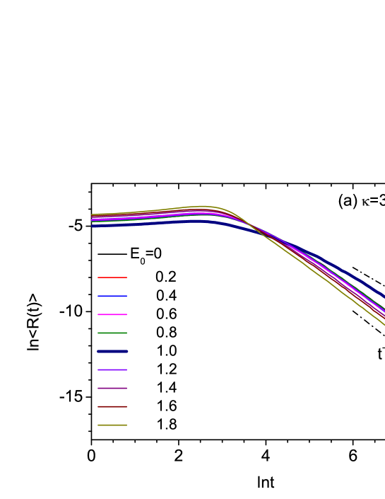


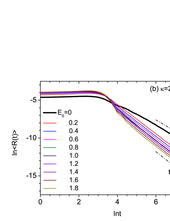
In Fig. 3, we set and plot the time evolution of for the same values of and as in Fig. 2. Similarly to the case, the localization behavior takes place for most values of , while the diffusive behavior appears only near a special value of . In contrast to the previous case, however, the diffusive behavior with is observed at . In addition, we have verified numerically that a similar diffusive behavior also occurs at , though it has not been shown here explicitly.
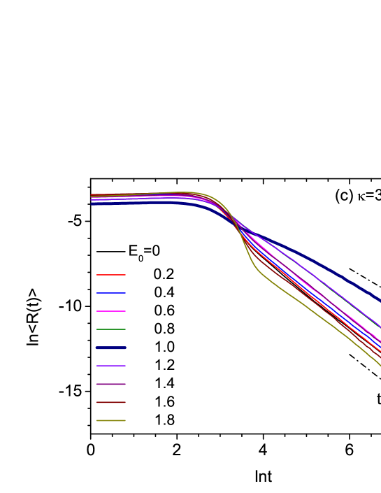
Next, in Fig. 4, we consider the case. The overall long-time behavior is similar to the and 3 cases, but the diffusive behavior with occurs at two different values and 1.4 () in the present case. In addition, a similar behavior is also observed at . Since the diffusive long-time behavior appears only in a narrow range of values, it can be considered as a kind of quasi-resonance. Combining the results obtained for , 3, and 4, we deduce that the quasi-resonances occur symmetrically with respect to and their total number is equal to . We also find that this behavior is unaffected by the disorder strength when .
In order to examine the quasi-resonant nature of the diffusive long-time behavior more clearly, we plot the exponent obtained by fitting the numerical results in the long-time region where versus , when , 3, 4, 5 and , 3, 4 in Fig. 5. We point out that there is a mirror symmetry in a statistical sense with respect to , though the region with is not shown here. Numerical results for many values around the sharp dips at , , and in addition to those shown in Figs. 2, 3, and 4 have been used in Fig. 5. As varies away from the values at the dips, increases rapidly from 1.5 to 2. The half-widths (full widths at half maximum) of all the dips are similar and roughly equal to 0.15. In order to show the positions of the quasi-resonances more clearly, some values of versus around the sharp dips are listed in Table 1.
| 0.90 | 1.778 | 1.30 | 1.822 | |
|---|---|---|---|---|
| 0.92 | 1.710 | 1.32 | 1.756 | |
| 0.94 | 1.636 | 1.34 | 1.680 | |
| 0.96 | 1.577 | 1.36 | 1.610 | |
| 0.98 | 1.534 | 1.38 | 1.554 | |
| 1.00 | 1.521 | 1.40 | 1.527 | |
| 1.02 | 1.535 | 1.42 | 1.510 | |
| 1.04 | 1.577 | 1.44 | 1.536 | |
| 1.06 | 1.640 | 1.46 | 1.580 | |
| 1.08 | 1.715 | 1.48 | 1.638 | |
| 1.10 | 1.786 | 1.50 | 1.710 |

In the rest of this subsection, we present some additional results which are useful in deducing a general formula for the quasi-resonant energy values. In Fig. 6, we plot versus at when , , 3, 4, 5, and 6, and . We find that the behavior of the incident wave packet at depends on the parity of . When is odd, the wave packet exhibits Anderson localization, while, when is even, it does a diffusive behavior.
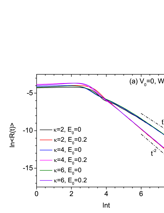
Finally, in Fig. 7, we compare the long-time scaling behavior at and 0.2, when and for , 4, and 6. A diffusive behavior is observed at when , while it is found at when . Therefore the quasi-resonance energy is found to depend on the value of as well as .


III.2 Quasi-resonant diffusion of wave packets
The numerical results presented above clearly show that a wave packet propagating inside a disordered mosaic lattice displays a diffusive behavior for some special values of the wave packet’s central energy in a quasi-resonant manner, although it exhibits Anderson localization for all the other values of the central energy. In other words, mosaic modulation of the lattice potential causes the usual exponential Anderson localization to be destroyed at special discrete values of the energy dependent on the modulation period. Thus we find that the periodic mosaic modulation is a feature that can induce a new type of delocaliztion in low-dimensional disordered systems.
From our numerical results given in the previous subsection, we can easily deduce that the central energy at the quasi-resonances, , is given precisely by
| (14) |
The number of is equal to . is distributed symmetrically with respect to and is included only when is even. For several small values of , we obtain
| (21) |
The analytical formula for the quasi-resonance energy appears to agree with the formula obtained for the resonance energy [e.g., Eq. (16) of Ref. 29] where the delocalization occurs in 1D binary random -mer models with . However, this agreement is only coincidental and superficial. In the binary random -mer model, the resonance energy has been obtained from the condition that the transmittance through a single -mer is unity, and therefore the transmittance at the resonance energies is identically equal to 1 and the corresponding states are completely extended [27, 28, 29, 30]. In contrast, at our quasi-resonance energies, the transmittance is not equal to 1 and the states are not extended but critical states, as will be explained in Sec. III.3. In the binary random -mer model of Ref. 29, the on-site potential can take one of the two values 0 and . The problem becomes nonrandom and trivial if and so we need to exclude that case. In order to have extended states, it is also necessary to have the condition that , which gives another constraint for [29]. On the contrary, in our model, is just a background on-site potential and can take any arbitrary value including zero. We also point out that the cosine form for the resonance energy of the -mer model arises only when the on-site potentials at all the sites of an -mer are the same. Even if they are not uniform, there can still exist resonance energies, but they will not be given by a simple cosine form.
We pay close attention to the results that the dependence of on shown in Fig. 5 is insensitive to the strength of disorder . In our model, the random potential is present only at periodically spaced sites (). In order for the numerical results to be insensitive to the disorder strength, it is natural to assume that the wave-function amplitudes take very small values close to zero at those sites. That is, the wave function has nodes there. This implies that the eigenfunctions have a periodicity with the wavelength satisfying
| (22) |
For such eigenfunctions, the energy eigenvalues should be very close to the values obtained in the disorder-free case, which are given by . Since the wave vector is related to by , we can obtain Eq. (14) in a straightforward way. This argument strongly suggests that the states at the energies are rather insensitive to the disorder and therefore are not standard exponentially localized states. Our conjecture that the wave functions at the quasi-resonance energies have nodes at will be confirmed later in Fig. 9 in Sec. III.3.
It is highly instructive to consider a related periodic model, which we may call periodic mosaic lattice model, defined by Eq. (4), but with replaced by a constant . Since this model is strictly periodic with a period , it contains alternating forbidden and allowed bands. In Fig. 8, we show its band structure when , , and . The gray-colored region denotes the forbidden bands. The dispersion relation between and is plotted in red inside the allowed bands. We have found that the energy values at the upper edges of the allowed bands are precisely given by Eq. (14) for all values of , , and . As the potential strength increases to large values, the widths of the allowed bands become very small. In the large limit, the allowed bands consist of infinitesimally narrow regions at the energies given by Eq. (14). If we compare this limiting case with the disordered mosaic lattice model for large , we find that the forbidden bands and the narrow allowed bands at in the periodic case are replaced respectively by exponentially localized states and diffusive states in the random case.

III.3 Nature of the states at the quasi-resonance energies
In order to better understand the nature of the states at the quasi-resonance energies, we digress briefly from the study of the time-dependent reflectance to consider the spectral properties of a finite disordered mosaic lattice. Specifically we calculate the participation ratio for the -th eigenstate with the energy eigenvalue , which is defined by [64]
| (23) |
where is the value of the -th eigenfunction at the site (). For a finite lattice, gives approximately the number of sites over which the -th eigenfunction is extended. To study the large- scaling behavior of the participation ratio in a disordered system, it is convenient to introduce a double-averaged quantity , where is obtained by averaging over all eigenstates within a narrow interval around and denotes averaging over a large number of independent disorder configurations. When is sufficiently large, we find a power-law scaling behavior of the form
| (24) |
with the scaling exponent . It has been well-established that for extended states, the scaling exponent is equal to 1 and increases linearly with increasing the lattice size . On the contrary, for (exponentially) localized states, the exponent is zero, that is, does not depend on and converges to a constant value as . For critical states at the boundary between extended and localized states, the exponent should be in the intermediate range of . Thus the finite-size scaling analysis of provides a very useful information about the nature of the states.
In Figs. 9(a) and 9(b), we show the results of numerical calculations of obtained when , , , 2, and the number of disorder configurations is 1000. In Fig. 9(a), we find that the average participation ratio for has pronounced peaks at the quasi-resonance energies , while it remains small at other energies. We have confirmed that for the value of away from , approaches a constant as increases to large values, implying that is zero and the states are exponentially localized. In contrast, at , is neither 0 nor 1 as demonstrated for in Fig. 9(b). From fitting the data to Eq. (24), we obtain for and for . These results clearly demonstrate that the states at the quasi-resonance energies are neither extended nor exponentially localized states. We notice that they closely resemble the critical states observed at Anderson localisation-delocalisation and quantum Hall plateau transitions [3, 65]. They are totally different from the resonant states appearing in the binary random -mer model, where such states have been found to be completely extended.
In Figs. 9(c) and 9(d), we illustrate the spatial distributions of the wave function amplitudes obtained for a single disorder configuration when , , , and , 1. When the energy is away from the quasi-resonance energies, we find that the wave function is strongly localized as in Fig. 9(c). At the quasi-resonance energies, however, the wave function has a distinct spatial distribution with several disjointed occupied regions as in Fig. 9(d). This is a unique characteristic frequently observed in critical or multifractal states. We also find that the wave function amplitudes are very close to zero at all the sites satisfying () as shown in the inset of Fig. 9(d), which is fully consistent with our conjecture that there are wave function nodes at such sites. This node structure is absent for localized wave functions and occurs only at the quasi-resonance energies. It leads to the behavior that when is sufficiently large, the quasi-resonant states are insensitive to the strength of disorder.
From separate calculations for the eigenfunctions of the periodic mosaic model, we have confirmed that they also have nodes at () only for the energies given by Eq. (14). Let us suppose that starting from the periodic mosaic model, we turn on the weak disorder at the sites () and increase its strength gradually. The special node structure of the wave function we have discussed so far will be maintained at the quasi-resonance energies regardless of the strength of disorder. Therefore the node structure of the wave functions is a crucial feature that connects the periodic and disordered mosaic lattice models and induces the critical states at the quasi-resonance energies. A more systematic and comprehensive analysis about the nature of the quasi-resonant states in the framework of the spectral problem will be presented elsewhere.
IV Conclusion
In this paper, we have studied numerically the time evolution of Gaussian wave packets in an effectively semi-infinite disordered mosaic lattice chain where the on-site potential takes a random value only at periodically spaced sites. We have performed extensive numerical calculations of the disorder-averaged time-dependent reflectance, , for various values of the wave packet’s central energy , the modulation period , and the disorder strength . We have found that the long-time behavior of obeys a power-law decay of the form in all cases. In the absence of the mosaic modulation (i.e., ), the exponent is equal to 2 regardless of the parameters, implying the onset of the standard Anderson localization. When the mosaic modulation is turned on (i.e., ), is still equal to 2 for almost all values of , while at a finite number (equal to ) of discrete values of dependent on , approaches 3/2, implying the onset of the classical diffusion. We have found that this phenomenon is independent of as long as it is sufficiently large and occurs in a quasi-resonant manner such that varies rapidly from 3/2 to 2 in a narrow energy range as varies away from the quasi-resonance values. We have deduced a simple analytical formula for the quasi-resonance energies and provided an explanation of this novel delocalization phenomenon based on the interplay between randomness and band structure and the node structure of the wave functions. We have also explored the nature of the states at the quasi-resonance energies using a finite-size scaling analysis of the average participation ratio and found that the states are neither extended nor exponentially localized, but ciritical states. The model proposed here can be readily realized experimentally using various physical systems, which include coupled optical waveguide arrays, synthetic photonic lattices, and ultracold atoms.
In the future research, it is desirable to perform a comprehensive spectral analysis of the participation ratio, the logarithmic transmittance, and the localization length to better elucidate the true nature of the states at the quasi-resonance energies as well as to test the theoretical predictions experimentally. Another interesting direction of research is to explore the spreading dynamics of a wave packet launched at the center of a long disordered mosaic lattice, which is expected to provide an understanding of the states at the quasi-resonance energies from a different perspective.
Acknowledgements.
B.P.N. would like to thank Felix Izrailev for carefully reading a draft version of the manuscript and providing valuable comments. We also appreciate greatly very helpful comments and suggestions by an anonymous referee and Seulong Kim. This research was supported through a National Research Foundation of Korea Grant (NRF-2022R1F1A1074463) funded by the Korean Government. It was also supported by the Basic Science Research Program funded by the Ministry of Education (2021R1A6A1A10044950) and by the Global Frontier Program (2014M3A6B3063708).References
- [1] P. W. Anderson, Absence of diffusion in certain random lattices, Phys. Rev. 109, 1492 (1958).
- [2] P. A. Lee and T. V. Ramakrishnan, Disordered electronic systems, Rev. Mod. Phys. 57, 287 (1985).
- [3] F. Evers and A. D. Mirlin, Anderson transitions, Rev. Mod. Phys. 80, 1355 (2008).
- [4] H. Hu, A. Strybulevych, J. H. Page, S. E. Skipetrov, and B. A. van Tiggelen, Localization of ultrasound in a three-dimensional elastic network, Nat. Phys. 4, 945 (2008).
- [5] G. Modugno, Anderson localization in Bose-Einstein condensates, Rep. Prog. Phys. 73, 102401 (2010).
- [6] S. A. Gredeskul, Y. S. Kivshar, A. A. Asatryan, K. Y. Bliokh, Y. P. Bliokh, V. D. Freilikher, and I. V. Shadrivov, Anderson localization in metamaterials and other complex media, Low Temp. Phys. 38, 570 (2012).
- [7] M. Segev, Y. Silberberg, and D. N. Christodoulides, Anderson localization of light, Nat. Photon. 7, 197 (2013).
- [8] R. R. Naraghi and A. Dogariu, Phase transitions in diffusion of light, Phys. Rev. Lett. 117, 263901 (2016).
- [9] D. Leykam, J. D. Bodyfelt, A. S. Desyatnikov, and S. Flach, Localization of weakly disordered flat band states, Eur. Phys. J. B 90, 1 (2017).
- [10] S. Derevyanko, Anderson localization of a one-dimensional quantum walker, Sci. Rep. 8, 1795 (2018).
- [11] Y. Sharabi, H. H. Sheinfux, Y. Sagi, G. Eisenstein, and M. Segev, Self-induced diffusion in disordered nonlinear photonic media, Phys. Rev. Lett. 121, 233901 (2018).
- [12] B. P. Nguyen, T. K. T. Lieu, and K. Kim, Numerical study of the transverse localization of waves in one-dimensional lattices with randomly distributed gain and loss: effect of disorder correlations, Waves Random Complex Media 32, 390 (2022).
- [13] P. Pelletier, D. Delande, V. Josse, A. Aspect, S. Mayboroda, D. N. Arnold, and M. Filoche, Spectral functions and localization-landscape theory in speckle potentials, Phys. Rev. A 105, 023314 (2022).
- [14] E. Abrahams, P. W. Anderson, D. C. Licciardello and T. V. Ramakrishnan, Scaling theory of localization: Absence of quantum diffusion in two dimensions, Phys. Rev. Lett. 42, 673 (1979).
- [15] J. E. Sipe, P. Sheng, B. S. White, and M. H. Cohen, Brewster anomalies: A polarization-induced delocalization effect, Phys. Rev. Lett. 60, 108 (1988).
- [16] K. Kim, F. Rotermund, D.-H. Lee, and H. Lim, Propagation of -polarized electromagnetic waves obliquely incident on stratified random media: Random phase approximation, Waves Random Complex Media 17, 43 (2007).
- [17] K. J. Lee and K. Kim, Universal shift of the Brewster angle and disorder-enhanced delocalization of waves in stratified random media, Opt. Express 19, 20817 (2011).
- [18] T. M. Jordan, J. C. Partridge, and N. W. Roberts, Suppression of Brewster delocalization anomalies in an alternating isotropic-birefringent random layered medium, Phys. Rev. B 88, 041105(R) (2013).
- [19] K. Kim, Anderson localization of electromagnetic waves in randomly-stratified magnetodielectric media with uniform impedance, Opt. Express 23, 14520 (2015).
- [20] K. Kim and S. Kim, Anderson localization and Brewster anomaly of electromagnetic waves in randomly-stratified anisotropic media, Mater. Res. Express 6, 085803(2019).
- [21] Q. Zhao, J. Gong, and C. A. Müller, Localization behavior of Dirac particles in disordered graphene superlattices, Phys. Rev. B 85, 104201 (2012).
- [22] A. Fang, Z. Q. Zhang, S. G. Louie, and C. T. Chan, Anomalous Anderson localization behaviors in disordered pseudospin systems, Proc. Natl. Acad. Sci. U.S.A. 114, 4087 (2017).
- [23] S. Kim and K. Kim, Anderson localization and delocalization of massless two-dimensional Dirac electrons in random one-dimensional scalar and vector potentials, Phys. Rev. B 99, 014205 (2019).
- [24] S. Kim and K. Kim, Anderson localization of two-dimensional massless pseudospin-1 Dirac particles in a correlated random one-dimensional scalar potential, Phys. Rev. B 100, 104201 (2019).
- [25] D. H. Dunlap, H.-L. Wu, and P. W. Phillips, Absence of localization in a random-dimer model, Phys. Rev. Lett. 65, 88 (1990).
- [26] V. Bellani, E. Diez, R. Hey, L. Toni, L. Tarricone, G. B. Parravicini, F. Domínguez-Adame, and R. Gómez-Alcalá, Experimental evidence of delocalized states in random dimer superlattices, Phys. Rev. Lett. 82, 2159 (1999).
- [27] H.-L. Wu, W. Goff, and P. W. Phillips, Insulator-metal transitions in random lattices containing symmetrical defects, Phys. Rev. B 45, 1623 (1992).
- [28] F. M. Izrailev, T. Kottos, and G. P. Tsironis, Hamiltonian map approach to resonant states in paired correlated binary alloys, Phys. Rev. B 52, 3274 (1995).
- [29] A. Kosior, J. Major, M. Płodzień, and J. Zakrzewski, Role of correlations and off-diagonal terms in binary disordered one-dimensional systems, Acta Phys. Pol. 128, 1002 (2015).
- [30] J. Major, Extended states in disordered one-dimensional systems in the presence of the generalized -mer correlations, Phys. Rev. A 94, 053613 (2016).
- [31] F. A. B. F. de Moura and M. L. Lyra, Delocalization in the 1D Anderson model with long-range correlated disorder, Phys. Rev. Lett. 81, 3735 (1998).
- [32] F. M. Izrailev and A. A. Krokhin, Localization and the mobility edge in one-dimensional potentials with correlated disorder, Phys. Rev. Lett. 82, 4062 (1999).
- [33] J. W. Kantelhardt, S. Russ, A. Bunde, S. Havlin, and I. Webman, Comment on “Delocalization in the 1D Anderson model with long-range correlated disorder”, Phys. Rev. Lett. 84, 198 (2000).
- [34] U. Kuhl, F. M. Izrailev and A. A. Krokhin, Experimental observation of the mobility edge in a waveguide with correlated disorder, Appl. Phys. Lett. 77, 633 (2000).
- [35] L. Sanchez-Palencia, D. Clement, P. Lugan, P. Bouyer, G.V. Shlyapnikov, and A. Aspect, Anderson localization of expanding Bose-Einstein condensates in random potentials, Phys. Rev. Lett. 98, 210401 (2007).
- [36] M. Piraud, P. Lugan, P. Bouyer, A. Aspect, and L. Sanchez-Palencia, Localization of a matter wave packet in a disordered potential, Phys. Rev. A 83, 031603(R) (2011).
- [37] J. Billy, V. Josse, Z. Zuo, A. Bernard, B. Hambrecht, P. Lugan, D. Clement, L. Sanchez-Palencia, P. Bouyer, and A. Aspect, Direct observation of Anderson localization of matter-waves in a controlled disorder, Nature 453, 891 (2008).
- [38] J. Biddle and S. Das Sarma, Predicted mobility edges in one-dimensional incommensurate optical lattices: An exactly solvable model of Anderson localization, Phys. Rev. Lett. 104, 070601 (2010).
- [39] A. Purkayastha, A. Dhar, and M. Kulkarni, Nonequilibrium phase diagram of a one-dimensional quasiperiodic system with a single-particle mobility edge, Phys. Rev. B 96, 180204(R) (2017).
- [40] H. P. Lüschen, S. Scherg, T. Kohlert, M. Schreiber, P. Bordia, X. Li, S. Das Sarma, and I. Bloch, Single-particle mobility edge in a one-dimensional quasiperiodic optical lattice, Phys. Rev. Lett. 120, 160404 (2018).
- [41] F. A. An, E. J. Meier, and B. Gadway, Engineering a flux-dependent mobility edge in disordered zigzag chains, Phys. Rev. X 8, 031045 (2018).
- [42] H. Yao, H. Khouldi, L. Bresque, and L. Sanchez-Palencia, Critical behavior and fractality in shallow one-dimensional quasi-periodic potentials, Phys. Rev. Lett. 123, 070405 (2019).
- [43] Y. Wang, X. Xia, L. Zhang, H. Ya, S. Chen, J. You, Q. Zhou and X.-J. Liu, One-dimensional quasiperiodic mosaic lattice with exact mobility edges, Phys. Rev. Lett. 125, 196604 (2020).
- [44] Q.-B. Zeng, R. Lü, and L. You, Topological superconductors in one-dimensional mosaic lattices, EPL 135, 17003 (2021).
- [45] Y. Liu, Y. Wang, X.-J. Liu, Q. Zhou, and S. Chen, Exact mobility edges, -symmetry breaking, and skin effect in one-dimensional non-Hermitian quasicrystals, Phys. Rev. B 103, 014203 (2021).
- [46] Q.-B. Zeng and R. Lü, Topological phases and Anderson localization in off-diagonal mosaic lattices, Phys. Rev. B 104, 064203 (2021).
- [47] L.-Y. Gong, H. Lu, and W.-W. Cheng, Exact mobility edges in 1D mosaic lattices inlaid with slowly varying potentials, Adv. Theory Simul. 4, 2100135 (2021).
- [48] Z.-H. Wang, F. Xu, L. Li, D.-H. Xu, and B. Wang, Topological superconductors and exact mobility edges in non-Hermitian quasicrystals, Phys. Rev. B 105, 024514 (2022).
- [49] D. Dwiputra and F.P. Zen, Single-particle mobility edge without disorder, Phys. Rev. B 105, L081110 (2022).
- [50] B. White, P. Sheng, Z. Q. Zhang, and G. Papanicolaou, Wave localization characteristics in the time domain, Phys. Rev. Lett. 59, 1918 (1987).
- [51] F. J. P. Schuurmans, M. Megens, D. Vanmaekelbergh, and A. Lagendijk, Light scattering near the localization transition in macroporous GaP networks, Phys. Rev. Lett. 83, 2183 (1999).
- [52] M. Titov and C. W. J. Beenakker, Signature of wave localization in the time dependence of a reflected pulse, Phys. Rev. Lett. 85, 3388 (2000).
- [53] P. M. Johnson, A. Imhof, B. P. J. Bret, J. G. Rivas, and A. Lagendijk, Time-resolved pulse propagation in a strongly scattering material, Phys. Rev. E 68, 016604 (2003).
- [54] S. E. Skipetrov and B. A. van Tiggelen, Dynamics of weakly localized waves, Phys. Rev. Lett. 92, 113901 (2004).
- [55] S. E. Skipetrov and B. A. van Tiggelen, Dynamics of Anderson localization in open 3D media, Phys. Rev. Lett. 96, 043902 (2006).
- [56] K. M. Douglass, S. John, T. Suezaki, G. A. Ozin, and A. Dogariu, Anomalous flow of light near a photonic crystal pseudo-gap, Opt. Express 19, 25320 (2011).
- [57] A. Aubry, L. A. Cobus, S. E. Skipetrov, B. A. van Tiggelen, A. Derode, and J. H. Page, Recurrent scattering and memory effect at the Anderson localization transition, Phys. Rev. Lett. 112, 043903 (2014).
- [58] S. E. Skipetrov and A. Sinha, Time-dependent reflection at the localization transition, Phys. Rev. B 97, 104202 (2018).
- [59] S. Aubry and G. André, Analyticity breaking and Anderson localization in incommensurate lattices, Ann. Isr. Phys. Soc. 3, 133 (1980).
- [60] T. Durduran, R. Choe, W. B. Baker, and A. G. Yodh, Diffuse optics for tissue monitoring and tomography, Rep. Prog. Phys. 73, 076701 (2010).
- [61] D. A. Boas and A. K. Dunn, Laser speckle contrast imaging in biomedical optics, J. Biomed. Opt. 15, 011109 (2010).
- [62] S. Shahjahan, A. Aubry, F. Rupin, B. Chassignole, and A. Derode, A random matrix approach to detect defects in a strongly scattering polycrystal: How the memory effect can help overcome multiple scattering, Appl. Phys. Lett. 104, 234105 (2014).
- [63] Diffuse Waves in Complex Media, edited by J.-P. Fouque (Kluwer, Dordrecht, 1999).
- [64] D. J. Thouless, Electrons in disordered systems and the theory of localization, Phys. Rep. 13, 93 (1974).
- [65] C. Castellani and L. Peliti, Multifractal wavefunction at the localisation threshold, J. Phys. A: Math. Gen. 19, L429 (1986).