Quantum traces for : The case
Abstract.
We generalize Bonahon–Wong’s -quantum trace map to the setting of . More precisely, given a non-zero complex parameter , we associate to each isotopy class of framed oriented links in a thickened punctured surface a Laurent polynomial in -deformations of the Fock–Goncharov -coordinates for higher Teichmüller space. This construction depends on a choice of ideal triangulation of the surface . Along the way, we propose a definition for a -version of this invariant.
1. Introduction
For a finitely generated group and a suitable Lie group , a primary object of study in low-dimensional geometry and topology is the -character variety
consisting of group homomorphisms from to , considered up to conjugation. Here, the quotient is taken in the algebraic geometric sense of geometric invariant theory [MFK94]. Character varieties can be explored using a wide variety of mathematical skill sets. Some examples include the Higgs bundle approach of Hitchin [Hit92], the dynamics approach of Labourie [Lab06], and the representation theory approach of Fock–Goncharov [FG06b].
In the case where the group is the fundamental group of a punctured surface of finite topological type with negative Euler characteristic, and where the Lie group is the special linear group, we are interested in studying a relationship between two competing deformation quantizations of the character variety , which we denote simply by . Here, a deformation quantization of a Poisson space is a family of non-commutative algebras parametrized by a non-zero complex parameter , such that the lack of commutativity in is infinitesimally measured in the semi-classical limit by the Poisson bracket of the space . In the case where is the character variety, the bracket is provided by the Goldman Poisson structure on [Gol84, Gol86, BG93].
The first quantization of the character variety is the -skein algebra of the surface ; see [Tur89, Wit89, Prz91, BFKB99, Kup96, Sik05, CKM14]. The skein algebra is motivated by the classical algebraic geometric approach to studying the character variety by means of its commutative algebra of regular functions . An example of a regular function is the trace function associated to a closed curve sending a representation to the trace of the matrix . A theorem of classical invariant theory, due to Procesi [Pro76], implies that the trace functions generate the algebra of functions as an algebra. According to the philosophy of Turaev and Witten, quantizations of the character variety should be of a 3-dimensional nature. Indeed, elements of the skein algebra are represented by (formal linear combinations of) knots (or links) in the thickened surface . The skein algebra has the advantage of being natural, but is difficult to work with in practice.
The second quantization of the -character variety is the Fock–Goncharov quantum space ; see [CF99, Kas98, FG09]. At the classical level, Fock–Goncharov [FG06b] introduced a framed version (also called the -moduli space) of the -character variety, which, roughly speaking, consists of representations equipped with additional linear algebraic data attached to the punctures of . Associated to each ideal triangulation of the punctured surface is a -coordinate chart for parametrized by non-zero complex coordinates where the integer depends only on the topology of the surface and the rank of the Lie group . When written in terms of these coordinates the trace functions on the character variety take the form of Laurent polynomials in -roots of the (a subtlety being that depends on the regular homotopy class of , represented by immersed curves, rather than the homotopy class of ). At the quantum level, there are -deformed versions of these coordinates, which no longer commute but -commute with each other, according to the underlying Poisson structure. The quantized character variety is obtained by gluing together quantum tori , including one for each triangulation consisting of Laurent polynomials in the quantized Fock–Goncharov coordinates . The quantum character variety has the advantage of being easier to work with than the skein algebra , but is less intrinsic.
We seek -deformed versions of the trace functions, associating to a closed curve a Laurent polynomial in the quantized Fock–Goncharov coordinates with respect to a fixed triangulation . Turaev and Witten’s philosophy leads us from the 2-dimensional setting of curves on the surface to the -dimensional setting of knots in the thickened surface . More precisely:
Conjecture 1 (-quantum trace map).
Fix a -root . For each ideal triangulation of the punctured surface (with empty boundary, ), there exists an injective algebra homomorphism
such that if , then for every blackboard-framed oriented knot in the thickened surface projecting to an immersed closed curve on the surface ,
This last equation says that the Fock–Goncharov classical trace polynomial associated to the curve is recovered in the classical limit. Moreover, the -quantum trace map should be natural, appropriately interpreted, with respect to the choice of triangulation ; see [Kim21].
Conjecture 1 is due to Chekhov–Fock [Foc97, CF00] in the case , and was proved ‘by hand’ in that case by Bonahon–Wong [BW11]. One of the motivations of the present work is to develop a conceptual understanding of their construction.
We prove the following, slightly weaker, version of Conjecture 1 in the case :
Theorem 2 (Theorem 22, -quantum trace polynomials).
Fix a -root . For each ideal triangulation of the punctured surface (with possibly non-empty boundary), there exists a function
such that if , then for every blackboard-framed oriented link whose components project to immersed closed oriented curves in ,
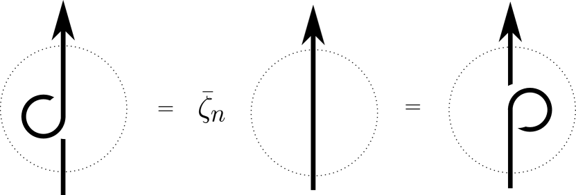
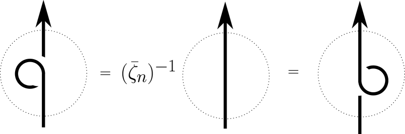
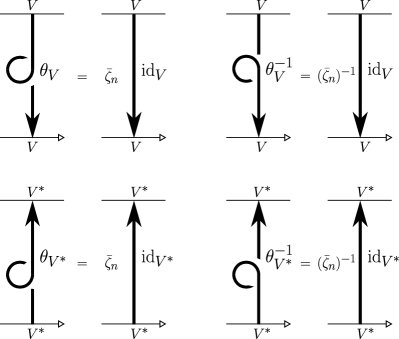
Moreover, this invariant satisfies the -evaluated HOMFLYPT relation [FYH+85, PT87], as well as the unknot and framing skein relations, for ; see Figures 1, 2, 3. In the figures, is the quantum integer, and is (essentially) the (co)ribbon element of the quantum special linear group (see Appendix A). ∎


In particular, the isotopy invariance property of Theorem 2 can be thought of as the main step toward proving Conjecture 1 in the case .
Theorem 2 was originally proved as part of [Dou20]. Our proof is also ‘by hand’, generalizing the strategy of [BW11], and relies on computer assistance for some of the calculations; see Appendix B.
Along the way, we propose a definition for a -version of the quantum trace polynomials; see §5.3. That this construction is well-defined for general is expected to follow from recent related work [CS23], which shares some overlap with [Dou21]; see Remark 37.
The solution of [BW11] in the case is implicitly related to the theory of the quantum group or, more precisely, of its Hopf dual ; see for instance [Kas95]. For general , we make this relationship more explicit; see §3.4 and Appendix A.
In addition to the HOMFLYPT relation, the skein algebra has other relations, best expressed as identities among certain -valent graphs in called webs [Kup96, Sik01, CKM14]. It is therefore desirable to extend the definition of the quantum trace polynomials from links to webs . Building on our construction for links, Kim [Kim20, Kim21] defined a -quantum trace map for webs, which is natural with respect to the choice of ideal triangulation . Combined with Kim’s work, the results of [DS24, DS20] lead to a proof of the injectivity property of Conjecture 1 in the case , which is closely related to the study of linear bases of skein algebras; see [DS24, §9.3].
As another application, Kim [Kim20] constructed a -quantum Fock–Goncharov duality map [FG09] (of the bangle, rather than bracelet, form [Thu14]), generalizing much of the solution of [AK17]; see also [All19, CKKO20]. For other related studies in the -setting, see [Hig23, FS22, IY23].
Lê–Yu [LY23] constructed a -quantum trace map for webs, agreeing at the level of links with the definition proposed in this paper. Their construction fits into a theory of -stated skein algebras [Lê18, CL22, LS21].
Quantum traces also appear in the context of spectral networks [Gab17, NY20]. Empirical computations performed together with A. Neitzke (see [NY22]) suggest that, at least for simple curves, the -quantum trace map defined in this paper agrees with that constructed in [NY22]; see also [KLS23] in the case .
Acknowledgements
This work would not have been possible without the guidance of my Ph.D. advisor Francis Bonahon. Many thanks go out to Sasha Shapiro and Thang Lê for informing me about related research and for enjoyable conversations, as well as to Dylan Allegretti and Zhe Sun who helped me fine-tune my ideas. I am also grateful to Andy Neitzke for sharing his enthusiasm for experiment, as well as to the referee for their helpful comments. Last but not least, Person D would like to thank Person G for their limitless support (and artistic inspiration).
2. Classical trace polynomials for
In this section, we will associate a Laurent polynomial in commuting formal -roots , , , to each immersed oriented closed curve transverse to a fixed ideal triangulation of a punctured surface , where depends only on the topology of and the rank of the Lie group .
2.1. Topological setup
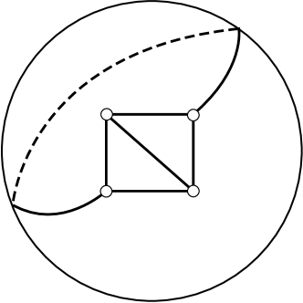
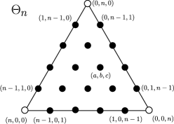
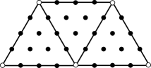
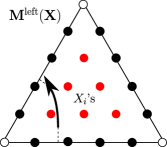
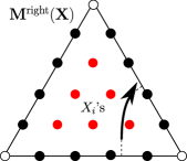
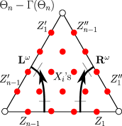
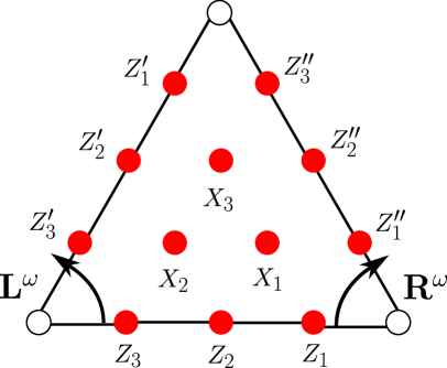
Let be an oriented punctured surface of finite topological type, namely is obtained by removing a finite subset , called the set of punctures, from a compact oriented surface . In particular, note that may have non-empty boundary, . We require that there is at least one puncture, that each component of is punctured (that is, intersects ), and that the Euler characteristic of the punctured surface satisfies where is the number of components of . Note that each component of is an ideal arc. These topological conditions guarantee the existence of an ideal triangulation of the punctured surface , namely a triangulation of the surface whose vertex set is equal to the set of punctures . See Figure 4 for some examples of ideal triangulations. The ideal triangulation consists of edges and triangles .
For simplicity, we always assume that does not contain any self-folded triangles. Consequently, each triangle of has three distinct edges. Such an ideal triangulation always exists (except when is a disk with one internal puncture and one puncture on the boundary). Our results should generalize to allow for self-folded triangles, requiring only minor adjustments (one would need to modify Definition 17–compare [BW11, §2.1], which makes use of the Weyl quantum ordering (§3.1.3)–but the main definition, Definition 35, is un-changed).
2.2. Discrete triangle
2.3. Dotted ideal triangulations
Let the punctured surface be equipped with an ideal triangulation , and let ; see §2.1.
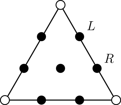
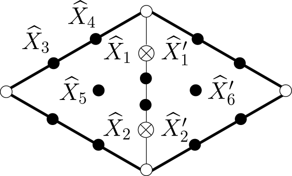
The associated dotted ideal triangulation consists of together with distinct black dots attached to the edges and triangles of , where there are edge-dots attached to each edge and triangle-dots attached to each triangle (punctures, that is, triangle vertices, are always drawn as white dots). For each triangle including its three boundary edges , , , these dots are arranged as the vertices of the discrete -triangle (minus its three corner vertices) overlaid on top of the ideal triangle ; see Figures 6 and 7. We talk about boundary-dots or interior-dots depending on whether the dots are on the boundary of interior of the surface.
Given a triangle of , which acquires an orientation from the orientation of , and given an edge of , it makes sense to say that an edge-dot on is to the left or to the right of another edge-dot on as viewed from the triangle ; see Figure 6(b).
We always assume that we have chosen an ordering for the dots lying on the dotted ideal triangulation , so we can talk about the -th dot, .
2.4. Classical polynomial algebra
Let the punctured surface be equipped with a dotted ideal triangulation .
Definition 3.
The classical polynomial algebra associated to the dotted ideal triangulation is the commutative algebra of Laurent polynomials generated by formal -roots and their inverses. We think of the generator as associated to the -th dot lying on . As for dots, see §2.3, we speak of edge- and triangle-generators as well as boundary- and interior-generators. Elements of are called coordinates. We often indicate edge-coordinates with the letter instead of .
Remark 4.
The algebraic coordinates in the classical polynomial algebra correspond to Fock–Goncharov’s geometric coordinates for the framed -character variety ; see §1. As a caveat, in the classical geometric setting the Fock–Goncharov coordinates are associated only to the interior-dots (not to the boundary-dots), while in the quantum algebraic setting there are coordinates associated to the boundary-dots as well.
In the language of cluster algebras [FZ02], these boundary-variables are also called frozen variables [FG06a, FG06b, FWZ16]. From the classical geometric point of view, one can think of the frozen boundary-coordinates as having the potential to become ‘actual’ un-frozen interior-coordinates if the surface-with-boundary were included inside the interior of a larger surface . At the quantum algebraic level, the inclusion of boundary-coordinates is an essential step in order to observe the local quantum properties; see, for instance, Theorem 16.
In the case of or , the Fock–Goncharov coordinates coincide with the shear or shear-bend coordinates for Teichmüller space due to Thurston [Thu97]; see [Bon96, Foc97, FG07a, HN16] for more details. There is also a geometric interpretation of Fock–Goncharov’s coordinates in the case , where the coordinates parametrize convex projective structures on the surface ; see [FG07b, CTT20].
2.5. Elementary edge and triangle matrices
Let denote the algebra of matrices with coefficients in the commutative classical polynomial algebra ; see Definition 9. Let the special linear group be the subset of consisting of the matrices with determinant equal to .
Let be an edge-coordinate in the classical polynomial algebra . For define the -th elementary edge matrix by
Note the normalizing factor multiplying the matrix on the left (or on the right). Similarly, for any triangle-coordinate in and for any index define the -th left elementary triangle matrix by
and define the -th right elementary triangle matrix by
Note that and do not actually involve the variable , so we will denote these matrices by and , respectively.
Remark 5.
In the theory of Fock–Goncharov, these elementary matrices for edges and triangles are called snake-move matrices. Each such matrix is the coordinate transformation matrix passing between a pair of compatibly normalized projective coordinate systems associated to a pair of adjacent snakes. For a framed local system in with coordinates , computing the monodromy of the local system around a curve amounts to multiplying together a sequence of snake-move matrices along the direction of the curve. For more details, see [FG06b, §9], [GMN14, Appendix A], and [Dou20, Chapter 2].
2.6. Local monodromy matrices
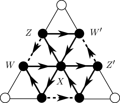
Let be a dotted ideal triangle, which we think of as sitting inside a larger dotted ideal triangulation ; see Figure 6. We assign matrices with coefficients in the classical polynomial algebra to various ‘short’ oriented arcs lying on the surface .
Recall that we think of the -discrete triangle (§2.2) as overlaid on top of the triangle , so that there is a one-to-one correspondence between coordinates in and vertices in (in other words, in the -discrete triangle minus its three corner vertices). Note that is a triangle-coordinate if and only if is an interior point , otherwise is an edge-coordinate.
We will use the following notational convention. Given an arbitrary family of matrices, put
First, consider a left-moving arc , as shown in Figure 8. We assume has no kinks (Figures 3(a) and 3(b)). Let be a vector consisting of the triangle-coordinates (Definition 3). Define the associated left matrix in by
where the matrix is the -th left elementary triangle matrix; see §2.5. (The dots colored red in the figure correspond to the coordinates appearing in the expression of the matrix associated to the curve.)
Next, consider a right-moving arc , as shown in Figure 9. We assume has no kinks. We define the associated right matrix in by
where the matrix is the -th right elementary triangle matrix; see §2.5.
Next, consider an edge-crossing arc , as shown on the left hand or right hand side of Figure 10. Let , , be the -th edge-coordinate (Definition 3), measured from right to left as seen by the triangle out of which the arc is moving. Let be a vector consisting of the ’s. Define the associated edge matrix in by
where the matrix is the -th elementary edge matrix; see §2.5. Note that if the orientation of the edge-crossing arc is reversed, then the edge matrix changes by permuting the coordinates by ; see Figure 10.
Observe that the order in which the elementary matrices are multiplied does not matter in the formula for the edge matrix , since they are diagonal, but does matter in the formulas for the triangle matrices and .
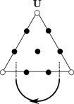
Lastly, define the clockwise U-turn matrix in by
We associate to a clockwise U-turn arc (resp. counterclockwise U-turn arc) , as shown on the left hand (resp. right hand) side of Figure 11, the U-turn matrix (resp. transpose of the U-turn matrix). Again, we have assumed that has no kinks. Note that (resp. ) when is even (resp. odd).
2.7. Definition of the -classical trace polynomials
Let be an immersed oriented closed curve in the surface such that is transverse to the ideal triangulation . We want to calculate the classical trace polynomial in associated to the immersed curve . We say that the polynomial is obtained from a ‘state sum’, ‘local-to-global’, or ‘transfer matrices’ construction.
More precisely, as we travel along the curve according to its orientation, assume crosses edges for in that order, and assume crosses triangles for in that order. As the curve crosses the edge , moving out of the triangle into the triangle , this defines an edge-crossing arc ; see §2.6 and Figure 10. Put and put
the associated edge matrix, where the are the edge-coordinates attached to the edge measured from right to left as seen from . As traverses the triangle between two edges and , it does one of three things:
-
•
the curve turns left, ending on , see Figure 8;
-
•
or turns right, ending on , see Figure 9;
-
•
or does a U-turn, thereby returning to the same edge , see Figure 11.
We also keep track of the following winding information: for the first and second items above, the number of full turns to the right that the curve makes while traversing the triangle ; and for the third item above, the number of half turns to the right that the curve makes before coming back to the same edge . Note . Note that the turning integer associated to the curve as it traverses the triangle will only be relevant when is even. Let the be the triangle-coordinates attached to the triangle , and put ; see Figure 8. Let be the curve obtained by ‘pulling tight’ the kinks of . (In particular, and are homotopic, but not, in general, regularly homotopic.) Corresponding to the three items above:
- •
- •
- •
In the first two cases, where is either left- or right-moving, put
and in the third case, where is a U-turn, put
where is the U-turn matrix defined in §2.6. Note, in the third case, that this is consistent with what was said in §2.6, where, in the case has no kinks, is associated to (resp. ) if travels clockwise hence (resp. counterclockwise hence ).
Definition 6.
The -classical trace polynomial associated to the immersed oriented closed curve , transverse to the ideal triangulation , is defined by
where on the right hand side we have taken the usual matrix trace. Note that this is independent of where one starts along the curve , by the conjugation invariance of the trace.
2.8. Relation to Fock–Goncharov theory
In this subsection, we assume (for simplicity) the surface has empty boundary, . A complete flag is a maximal nested sequence of distinct sub-spaces . The group acts on the set of complete flags by matrix multiplication.
In [FG06b], Fock–Goncharov define the moduli space of framed local systems, also called the -moduli space, whose complex points have been denoted in this paper by . A framed local system over is, roughly speaking, a pair where is a group homomorphism and assigns to each puncture a complete flag invariant under the monodromy of any peripheral curve around , that is, . Framed local systems are considered up to equivalence under the action of , which in particular acts on representations by conjugation.
Fock–Goncharov associate to each ideal triangulation of a coordinate chart for the moduli space parametrized by non-zero complex coordinates . Here, is the number of dots associated to the ideal triangulation ; see §2.3, 2.4. In particular, choosing and -many coordinates determines a representation up to conjugation. Since is valued in , the trace for any is well-defined only up to multiplication by a -root of unity.
Theorem 7 ([FG06b], -classical trace polynomials).
Fix an ideal triangulation of the punctured surface . Let be a representation given by Fock–Goncharov coordinates as above. Moreover, choose arbitrary -roots . Then for each immersed oriented closed curve in transverse to the ideal triangulation , the trace equals the evaluated classical trace polynomial (Definition 6) up to multiplication by a -root of unity. ∎
3. Quantum matrices for
In this section, we will define quantum versions of the classical polynomial algebra and the classical local monodromy matrices, and relate them to the quantum special linear group . Throughout, let and be a -root of . Technically, also choose .
3.1. Quantum tori, matrix algebras, and the Weyl quantum ordering
3.1.1. Quantum tori
For a natural number , let (for ‘Poisson’) be an integer anti-symmetric matrix.
Definition 8.
The quantum torus (with -roots) associated to is the quotient of the free algebra in the indeterminates by the two-sided ideal generated by the relations
Put . We refer to the as generators, and the as quantum coordinates, or just coordinates. Define the subset of fractions
Written in terms of the coordinates and the fractions , the relations above become
3.1.2. Matrix algebras
Definition 9.
Let be a, possibly non-commutative, algebra, and let be a positive integer. The matrix algebra with coefficients in , denoted , is the complex vector space of matrices, equipped with the usual multiplicative structure. Specifically, the product of two matrices and is defined entry-wise by
As usual, the entry of a matrix is the entry in the -th row and -th column. Note that the order of and in the above equation matters since these elements might not commute in .
3.1.3. Weyl quantum ordering
If is a quantum torus (§3.1.1), then there is a linear map
from the free algebra to , called the Weyl quantum ordering, defined by the property that a word for (note may equal if ) is mapped to
Also, the empty word is mapped to . Note the Weyl ordering depends on the choice of ; see the beginning of §3. The Weyl ordering is specially designed to satisfy the symmetry
for every permutation of . Also, . Let
be the induced linear map from the commutative Laurent polynomial algebra to . This determines a linear map of matrix algebras
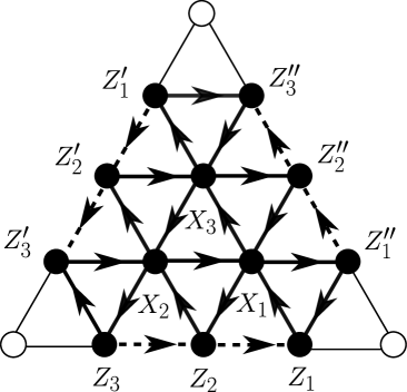
3.2. Fock–Goncharov quantum torus for a triangle
Let denote the set of corner vertices of the discrete triangle ; see §2.2.
Define a function
using the quiver with vertex set illustrated in Figure 12. The function is defined by sending the ordered tuple of vertices of to (resp. ) if there is a solid arrow pointing from to (resp. to ), to (resp. ) if there is a dotted arrow pointing from to (resp. to ), and to if there is no arrow connecting and . Note that internal arrows are solid, and boundary arrows are dotted. By labeling the vertices of by their coordinates we may think of the function as a anti-symmetric matrix called the Poisson matrix associated to the quiver. Here, ; see §2.3.
Definition 10.
The Fock–Goncharov quantum torus , also denoted , associated to the triangle is defined to be the quantum torus determined by the Poisson matrix , with generators for all . Note that when this recovers the classical polynomial algebra for ; see §2.4.
As a notational convention, for we write (resp. and ) in place of (resp. and ); see Figure 13. So, triangle-coordinates will be denoted for while edge-coordinates will be denoted .
Remark 11.
Intuitively speaking, we think of the -coordinates as quantizations of ‘half’ of their corresponding classical edge-coordinates. This is because the ‘other half’ of each coordinate lives in an adjacent triangle. When viewed inside an ideal triangulation , an edge of ‘splits’ this classical edge-coordinate into its two ‘quantum halves’. Compare Figure 16.
3.3. Quantum left and right matrices
Although the general (global) definition of the -quantum trace polynomials (§5.3) is somewhat technical (requiring that one keep track of the ordering of the non-commuting quantum torus variables), the extension of the local monodromy matrices (§2.6) to the quantum setting is more straightforward, just using the Weyl quantum ordering (§3.1.3) to symmetrize the variables.
3.3.1. Weyl quantum ordering for the Fock–Goncharov quantum torus
Let be the Fock–Goncharov quantum torus (§. Then the Weyl ordering of §3.1.3 gives a map
where we have used the identification discussed in §3.2.
3.3.2. Quantum left and right matrices
Let be a triangle. An extended left-moving arc is similar to a left-moving arc, from §2.6, except that it extends all the way to the two distinct edges of the triangle ; see Figure 13. We think of an extended left-moving arc as the concatenation of ‘half’ of an edge-crossing arc together with a left-moving arc together with another half of an edge-crossing arc , as indicated in Figure 13; compare Remark 11. We refer to these halves of edge-crossing arcs as half-edge-crossing arcs. Similarly, we define extended right-moving arcs .
Defined as in §2.6 are left matrices , right matrices , and edge matrices in associated to non-extended left-moving arcs (Figure 8), non-extended right-moving arcs (Figure 9), and half-edge-crossing arcs, respectively.
Definition 12.
Put vectors , , , and as in Figure 13. To an extended left-moving arc , as in Figure 13, we associate a quantum left matrix in by the formula
where we have applied the Weyl quantum ordering discussed in §3.3.1 to the product of classical matrices in (actually, in ). This just means that we apply the Weyl ordering to each entry of the classical matrix. Similarly, to an extended right-moving arc , as in Figure 13, we associate a quantum right matrix in by the formula
3.4. Quantum and its points: first result
(For a more theoretical discussion about quantum , see Appendix A.) Let be a, possibly non-commutative, algebra.
Definition 13.
A matrix in is a -point of the quantum matrix algebra , denoted , if
| () |
A matrix is a -point of the quantum special linear group , denoted , if and the quantum determinant
These notions are also defined for matrices, as follows.
Definition 14.
A matrix is a -point of the quantum matrix algebra , denoted , if every submatrix of is a -point of . That is,
for all and , where . A matrix is a -point of the quantum special linear group , denoted , if both and . Here, the quantum determinant of a matrix is
where the length of the permutation is the minimum number of factors appearing in a decomposition of as a product of adjacent transpositions ; see, for example, [BG02, Chapter I.2].
Remark 15.
Note that the definitions satisfy the property that if a -point is a triangular matrix, then the diagonal entries commute, and .
Note also that the subsets and are generally not closed under matrix multiplication.
Take to be the Fock–Goncharov quantum torus for the triangle , as defined in §3.2. Let and in be the quantum left and right matrices, respectively, as defined in Definition 12. In a companion paper, we prove:
Theorem 16 ([Dou21], -quantum matrices).
The quantum left and right matrices,
are -points of the quantum special linear group . That is, . ∎
3.5. Examples
3.5.1. example.
Consider the case ; see Figure 14. On the right hand side, we show the quiver defining the commutation relations in the quantum torus , recalling Figure 12 and the definitions of §3.1.1 and 3.2. For instance, the following are some sample commutation relations:
Then, the quantum left and right matrices are computed as
and
Theorem 16 says that these two matrices are elements of . For instance, the entries of the sub-matrix of ,
satisfy Equation ( ‣ 13). For a computer verification of this, see Appendix B. We also demonstrate in the appendix that Equation ( ‣ 13) is satisfied by the entries of the sub-matrix of ,
3.5.2. example.
Consider the case ; see Figure 15. On the right hand side, we show the quiver defining the commutation relations in the quantum torus , recalling Figure 12 and the definitions of §3.1.1 and 3.2. For instance, the following are some sample commutation relations:
Then, the quantum left and right matrices are computed as
and
Theorem 16 says that these two matrices are elements of . For instance, the entries of the sub-matrix (arranged as a matrix) of ,
satisfy Equation ( ‣ 13). For a computer verification of this, see Appendix B. We also demonstrate in the appendix that Equation ( ‣ 13) is satisfied by the entries of the sub-matrix (arranged as a matrix) of ,
3.6. Quantum tori for surfaces
For a dotted ideal triangulation of , in §2.4 we defined the classical polynomial algebra where there is one generator associated to every dot on . In the case where is an ideal triangle, in §3.2 we deformed the classical polynomial algebra to a quantum torus . We now generalize the quantum torus to a quantum torus associated to the triangulated surface which deforms the classical polynomial algebra .
For each dotted triangle of , associate a copy of , which is also a dotted triangle, such as that shown in Figure 6(b). Note that the boundary consists of three ideal edges. The dotted ideal triangulation can be reconstructed from the individual triangles by supplying additional gluing data. To each dotted triangle associate the Fock–Goncharov quantum torus of the triangle , whose coordinates we will denote by . Recall that a generator of the quantum torus is either a triangle-generator or an edge-generator. If is an edge-generator, then there are two cases:
-
•
the corresponding generator in the classical polynomial algebra for the glued surface is a boundary-generator;
-
•
the corresponding generator in is an interior-generator.
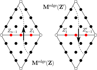
In the second case, the corresponding interior-generator in lies on an internal edge of the ideal triangulation . So, there exists a triangle adjacent to along the edge . Moreover, there exists a unique edge-generator in the quantum torus for the triangle that also corresponds to the interior-generator in lying on the internal edge . Therefore, we may say that the two quantum generators in and in correspond to one another; see Figure 16.
Definition 17.
The Fock–Goncharov quantum torus associated to the surface equipped with the dotted ideal triangulation is the sub-algebra,
of the tensor product of the Fock–Goncharov quantum tori associated to the copies of the dotted triangles of the ideal triangulation , generated:
-
•
by triangle-generators in ;
-
•
by tensor products in of corresponding edge-generators associated to a common internal edge lying between two triangles and in ;
-
•
and by edge-generators in associated to boundary edges of .
In particular, when , the Fock–Goncharov quantum torus is naturally isomorphic to the classical polynomial algebra (as indicated by the notation). (Going forward, we will omit the ‘hat’ symbol in the notation, naturally identifying triangles with .)
Remark 18.
An important difference between the local quantum tori for the triangles and the global quantum torus for the triangulated surface is that two edge-generators and in lying on the same boundary edge of may not commute, rather may -commute, while the corresponding interior-generators and in always commute. This is because the orientations of the two triangles’ and quivers go against each other (Figures 12, 16). Intuitively, the local -commutation relations on the boundary are created upon ‘splitting the edge-coordinates in half’ at the quantum level (Remarks 4, 11). This phenomenon does not occur for because there each edge carries only one coordinate.
4. Main theorem: quantum trace polynomials for
4.1. Framed oriented links in thickened surfaces
So far, we have been working in the 2-dimensional setting of the punctured surface . We now turn to the 3-dimensional setting of the thickened surface . We will follow [BW11, §3.1], the only difference being that we consider oriented links.
Definition 19.
A framed oriented link in the thickened surface is a compact oriented one-dimensional manifold, possibly-with-boundary, that is embedded in and is equipped with a framing (see below), satisfying the following properties:
-
•
we have ;
-
•
the framing at a boundary point of is vertical, meaning parallel to the axis and pointing in the direction (or, in pictures, toward the eye of the reader);
-
•
for each boundary component of , the finitely many points have distinct heights, meaning that the coordinates with respect to are distinct.
Here, by a framing, we mean the choice of a smooth assignment along the link of unit vectors in the tangent spaces of such that this vector field on is everywhere orthogonal to . A framed oriented knot is a closed framed oriented link (namely, a framed oriented link with empty boundary ) with one connected component. Two framed oriented links and are isotopic if can be smoothly deformed to through the class of framed oriented links. By possibly introducing kinks (Figures 3(a) and 3(b)), one can always isotope a framed link so that it has blackboard framing, meaning constant vertical framing in the direction (with respect to the coordinate).
Remark 20.
We display links in figures by their diagrams, namely their projections onto the surface equipped with over/under crossing information. By convention, all link diagrams represent blackboard-framed links.
Instead of using the picture conventions of [BW11, §3.5], in our diagrams we will indicate explicitly which points lying on a single boundary component of are higher or lower with respect to the direction. (Note, importantly, that two points of on a single boundary component cannot exchange heights during an isotopy of the link.)
One can think of a framed link as a ‘ribbon’, namely an oriented annulus (that is, oriented as a surface, not to be confused with link orientations) embedded in where the framing is perpendicular to the annulus and determined by the orientation.
4.2. Stated links
Definition 21.
A (-)stated framed oriented link is a framed oriented link equipped with a function
called the state, assigning to each element of the boundary of the link a state-number in (we often confuse ‘state’ with these state-numbers). Note that a stated closed link is the same thing as a closed link. As for links, there is the corresponding notion of isotopy of stated links.
Let be a stated framed oriented link in a triangulated surface obtained by gluing together two triangulated surfaces and along edges of the triangulations. Let and be the associated links in and . We say states and for stated links and such that and agree with on are compatible if their values agree on the common boundaries of and (resulting from cutting ).
4.3. Main result
In this subsection, we restrict to the case . Let the surface be equipped with a dotted ideal triangulation . Recall the Fock–Goncharov quantum torus associated to this data; see Definition 17.
Note that if is a blackboard-framed oriented knot (meaning, in particular, that it is closed), and if is the natural projection, then, possibly after an arbitrarily small perturbation of the knot , we have that is an immersed oriented closed curve in , so we may consider the classical trace polynomial in associated to ; see Definition 6.
We now give a more detailed version of Theorem 2 from §1. Technically, our solution involves choosing a square root of the parameter . Proofs will be given in §5, 6.
Theorem 22 (-quantum trace polynomials).
Let be a non-zero complex number, and let be a -root of ; choose also . There is a function
satisfying the following properties:
-
(A)
the element is invariant under isotopy of stated framed oriented links;
-
(B)
the -HOMFLYPT skein relation (Figure 1 with ) holds;
- (C)
Complement 23.
Moreover, this invariant satisfies the following additional properties.
-
•
(Classical Trace Property) Let and let be a closed blackboard-framed oriented knot. Then,
where is the immersed oriented closed curve obtained by projecting to .
-
•
(Multiplication Property) Let be a stated framed oriented link, written as a disjoint union of links . Assume in addition that lies entirely below in , with respect to the height coordinate. Then,
Note that the order of multiplication matters, since is non-commutative.
-
•
(State Sum Property) Let be a stated framed oriented link in a triangulated surface obtained by gluing together two triangulated surfaces and . Let and be the associated links in and . Then,
5. Quantum trace polynomials for
The corresponding version of Theorem 22 and Complement 23 should hold in the case of , by replacing with everywhere in the statement. In this section, we will construct the quantum trace map for general . However, we only give a proof that it is well-defined for . For concreteness, along the way we will give explicit formulas for the case . When , our construction coincides with that in [BW11]. In particular, our construction gives a way to think of their construction, which was defined for un-oriented links, in terms of oriented links. Throughout, fix and a -root of . Technically, also choose .
5.1. Matrix conventions
We will need to display and matrices. Lower indices will indicate rows and upper indices will indicate columns. A matrix will be displayed in the general form
A matrix will be displayed in the general form
If and are finite-dimensional complex vector spaces with bases and and if is a linear map, we define the matrix associated to and these bases of and by the property
5.2. Biangle quantum trace map
A biangle is a closed disk with two punctures on its boundary. Biangles do not admit ideal triangulations, so is never a biangle. However, we may still consider stated framed oriented links in the thickened biangle defined just as before. In this subsection, we will (implicitly) use the Reshetikhin–Turaev construction [RT90] to provide an analogue of Theorem 22 and Complement 23 for biangles, valued in the complex numbers ; see Appendix A for the explicit (and more conceptual) connection to [RT90]. Note that this subsection does not require the choice of square root .
Parametrize the thickened biangle such that, in Figure 17(a) say, the first coordinate points along the page to the right, the second coordinate points along the page up, and the third coordinate points out of the page toward the eye of the reader. Note this parametrization is not canonical: there are two possibilities, related by ‘turning the biangle on its head’. The construction will be independent of this choice of parametrization (see the comments after Proposition 30).
In order to state the result, we first define some elementary matrices associated to certain local link diagrams, namely various U-turns and crossings.
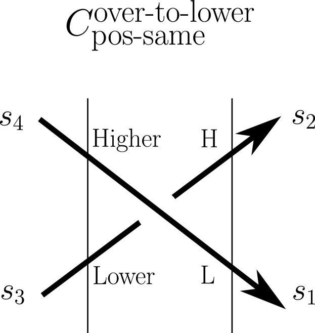
5.2.1. U-turns
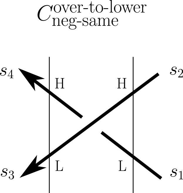
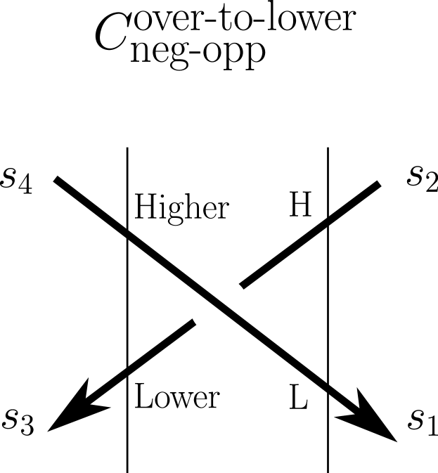
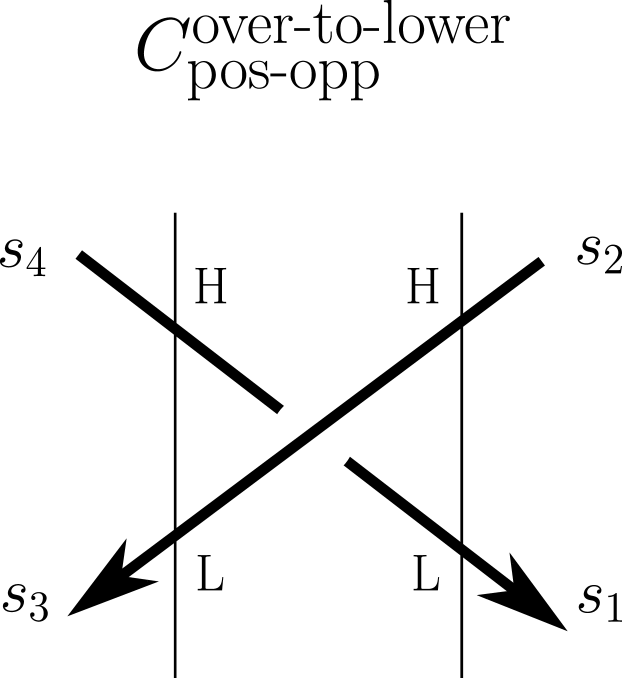
In Figures 17 and 18, we show the four possible U-turns, which are in particular stated framed oriented links with the blackboard framing. In agreement with our picture conventions (see Remark 20), the boundary point of the link that is labeled ‘Higher’ or ‘H’ is higher, namely has a greater coordinate with respect to the direction, than the boundary point of the link that is labeled ‘Lower’ or ‘L’.
Definition 24.
-
•
The -coribbon element is
(Note the overbar notation in does not mean ‘complex conjugation’.) For the categorical context, see §A.3.2.
-
•
Define the square root of the (signed) coribbon element by
We require the parenthetical ‘signed’ because we can only say . Note that is always even, so here we do not need to choose a square root .
-
•
Define a matrix over the complex numbers by
where it is implicit that we are putting as above, so is defined. Note that the common ratio between adjacent entries in the matrix is equal to . Note also that putting recovers the classical U-turn matrix from §2.6. For example, in the case , the matrix is
Definition 25.
For each pair of states , define four complex numbers
by the matrix equations
see §5.1. Here, the superscript indicates that we are taking the matrix transpose. For example, in the case , in the above formulas .
Remark 26.


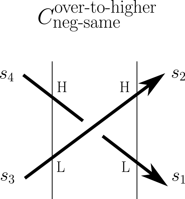
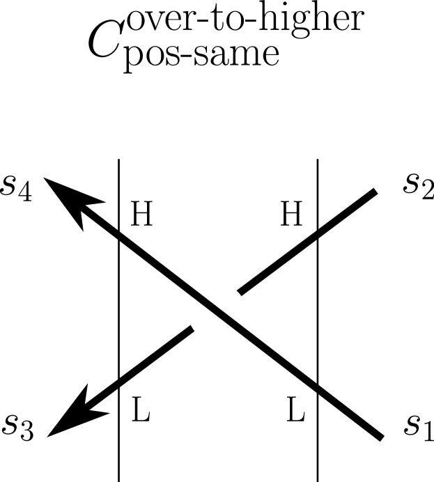
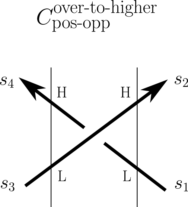
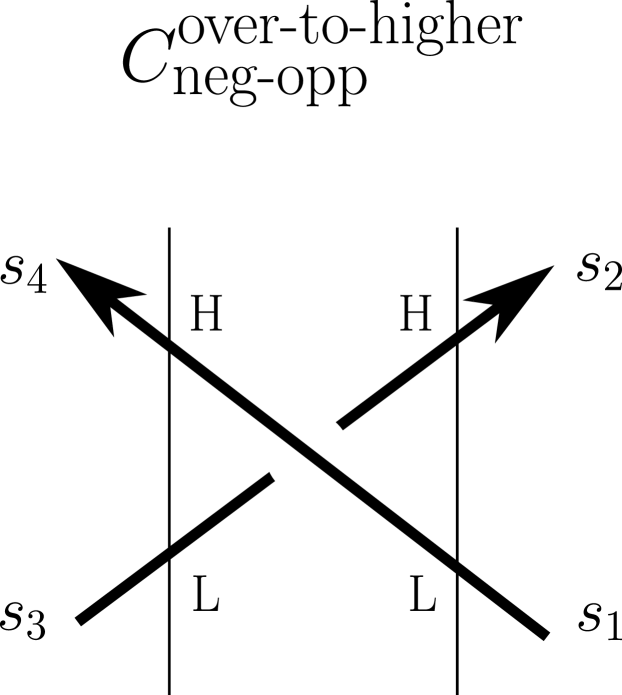
5.2.2. Crossings
Shown in Figures 19 and 20 are the eight possible crossings, with blackboard framing and the usual picture conventions as above.
Let be a -dimensional complex vector space, and let be the complex vector space dual to . Choose a linear basis for , and let be the corresponding dual basis for . Define four linear isomorphisms
by extending linearly the following assignments for tensor product basis elements
Define bases , , , and of , , , and by
For example, when , the ordered basis is .
The following fact, a simple calculation from the above definitions, motivates the definitions of the matrices and below (and will be used in Appendix A).
Fact 27.
We have the following equalities of matrices
representing the linear isomorphisms , , and when expressed in terms of the bases , , and . Also, these matrices are symmetric. ∎
For example, in the case , these two matrices and are given by
An observation is that, for general , when then the two matrices and are identical. For another property of these -matrices, see §5.4.1.
Definition 28.
For each quadruple of states , define eight complex numbers
by the matrix equations
Remark 29.
In the case , these formulas agree with those in [BW11, Lemma 22], for the underlying un-oriented link, taking , and (see [BW11, Proposition 26]). In particular, as another indication of the un-oriented nature of , when the two matrices and are identical for all and (we saw above that, for general , this is only true for ). This can be explained conceptually as follows. For any , the vector spaces and can be given the structure of a right -comodule; see Appendix A. When , the linear isomorphism , , is an isomorphism of right -comodules, but this is not true for . This is why, loosely speaking, the choices above for the bases , , and are ‘preferred’.
The linear isomorphisms , , and arise naturally as braidings in the ribbon category of finite-dimensional right -comodules, where the categorical coribbon element is essentially given by Definition 24; see Appendix A. Possibly of interest, we have implicitly taken a ‘symmetric’ duality, which is more fitting for the current setting. In the notation of [Kas95] (compare [Kas95, Chapter XIV.2, Example 1]), these symmetric dualities and are related to the usual ones by and , where ; see Appendix A. Note that is the bottom left entry of , see Definition 24.
5.2.3. Trivial strand
Consider a single strand crossing from one boundary edge of the biangle to the other boundary edge, as shown in Figure 21. Note that the height of the strand with respect to the component does not play a role in this particular case.
This trivial strand corresponds to the identity matrix. That is, define for each pair of states the complex number by the matrix equation

5.2.4. Kinks and the biangle quantum trace map
Up to this point, we have assigned complex numbers to a handful of small stated blackboard-framed oriented links (but not their isotopy classes) in the parametrized (see the beginning of §5.2) thickened biangle . We now provide the general assignment.
Assume first that the blackboard-framed link has no kinks. For the moment, we also assume that higher points of (resp. ) have larger second coordinates with respect to the parametrization of ; see, for example, Figures 17, 18, 19, 20. (Recall, in particular, Remark 20.) Fixing endpoints, isotope (without introducing kinks) into an arbitrary bridge position. This means that, after isotopy, there exists a partition of such that is a disjoint union of links satisfying:
-
•
the higher points of have a larger second coordinate;
- •
(Compare [BW11, §4, proof of Lemma 15].) For each and any state on , define
see §5.2.1, 5.2.2, 5.2.3. We then define the number
Here, the states are compatible (Definition 21) if and
and .
Define for a general stated blackboard-framed oriented link , possibly with kinks (§4.1), as follows. By isotopy, sliding the link horizontally along the boundary of while preserving blackboard framing throughout, we can arrange that the boundary satisfies the ‘higher point, larger second coordinate’ condition assumed just above. (Note this sliding might introduce or remove kinks.) Let be the blackboard-framed link without kinks obtained by removing the kinks of (more precisely, pulling tight by homotopy–not isotopy–the kinks in the un-framed link underlying ), and further isotoped into a bridge position as above. Then we have defined a complex number . Define by modifying according to the un-kinking ‘skein relations’ shown in Figures 3(a) and 3(b). (For example, in the case , .) More precisely, for (resp. ) the number of positive (resp. negative) kinks of ,
Proposition 30 (-biangle quantum trace map).
Let be the (non-parametrized) thickened biangle. Then the construction of the current section determines a function
satisfying the following properties:
-
(A)
the number is invariant under isotopy of stated framed oriented links;
-
(B)
the -HOMFLYPT skein relation (Figure 1) holds;
- (C)
Moreover, this invariant satisfies the Multiplication Property
in the case where is the disjoint union of links having mutually non-overlapping heights (note the order of multiplication is immaterial, in contrast to Complement 23), as well as the State Sum Property
where and are the links obtained by cutting the biangle into two biangles and .
For the proof of part (A) of the proposition, namely the isotopy invariance, we refer the reader to Appendix A, which makes use of a ‘symmetric’ specialization of the Reshetikhin–Turaev invariant (see Figure 41). The skein relations, parts (B) and (C), are local calculations; see §5.4.1.
Note that (assuming isotopy invariance) the State Sum Property is immediate from the construction. It suffices to establish the Multiplication Property when (assuming lies below , say). This follows from the State Sum Property and the definition for the trivial strand (Figure 21) by choosing a parametrization of , the partition of , and a position for the links such that (resp. ) with only trivial strands in (resp. ). (Compare [BW11, Lemma 19].)
We note, in particular, that the biangle quantum trace map is independent of the choice of parametrization of the biangle , discussed at the beginning of §5.2. Indeed, this property follows either from the properties of the symmetric specialization of the Reshetikhin–Turaev invariant (Appendix A), or directly from the symmetries of the matrices corresponding to the links displayed in Figures 17, 18, 19, 20, 21.
Remark 31.
The Reshetikhin–Turaev invariant can be defined more generally for ribbon graphs, including so-called webs [Kup96, Sik05]. In [BW11], the -quantum trace is defined by splitting the edges of the ideal triangulation to form biangles and then “pushing all of the complexities of the link into the biangles,” [BW11, p.1596] leaving only flat arcs lying over the triangles. In order to construct the -quantum trace for webs, one can perform the same procedure, in particular pushing all of the vertices of the web into the biangles. Then, the Reshetikhin–Turaev invariant can be applied to the webs in the biangles and (as we will see in the next section) the Fock–Goncharov matrices can be associated to the arcs lying over the triangles. This is essentially the strategy employed in [Kim20] in the case .
5.3. Definition of the -quantum trace polynomials
Our construction of the quantum trace map in the general case will follow exactly the same procedure as explained in [BW11, §3.4-6] for the case , where our Proposition 30 plays the role of Proposition 13 in [BW11, §4]. It remains to discuss how Property (2)(a) of Theorem 11 in [BW11, §3.4], concerning the values of the quantum traces for arcs in triangles (see Remark 31), generalizes to our setting, which we have essentially already done. (In particular, we follow the ‘ordered lower to higher, multiply left to right’ convention of [BW11] for ordering the non-commutative variables associated to different arc components lying over a single triangle.) After this, the rest of the construction is identical to [BW11, §6, pp. 1600-1601], where the quantum trace for a general triangulated surface is defined as a state sum over the triangles of the ideal triangulation of . We proceed below to spell all of this out in greater detail. Now is the point where we require the choice of square root ; see Remark 33.
5.3.1. Arcs in a triangle
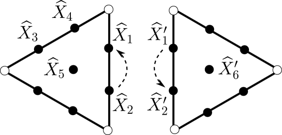
Generalizing Property (2)(a) of Theorem 11 in [BW11, §3.4] to the case of general is accomplished by using the quantum left and right matrices and , with coefficients in the Fock–Goncharov quantum torus for a triangle in the ideal triangulation , appearing earlier in Theorem 16.
Consider a single extended left-moving or right-moving arc crossing the triangle between two distinct boundary edges, such as those shown in Figure 13; see §3.3.2. For example, in the case , these extended left-moving and right-moving arcs are displayed in Figures 22(a) and 22(b). Using the notation from these figures, the quantum left and right matrices and are given by
where in is defined by
and
where in is defined by
(This is the result of multiplying out the snake-move matrices in the case ; compare §3.5.1.)
Definition 32.
For general , define for each pair of states two elements in the quantum torus
by the matrix equations (see §5.1)
Remark 33.
In the above matrices, we recall that the square brackets surrounding the monomials indicate that we are taking the Weyl quantum ordering, which depends on the quiver defining the -commutation relations in the Fock–Goncharov quantum torus ; see §3.1.3 and Figure 12. It is here that the choice of enters into the construction.
In Theorem 16, we saw that the quantum left and right matrices and are points of the quantum special linear group . Note that, in order for these matrices to satisfy even just the relations required to be in the quantum matrix algebra , they had to be normalized by ‘dividing out’ their determinants. For example, the above version of the matrix would not satisfy the -commutation relations required to be a point of if we had instead put .
5.3.2. Good position of a link
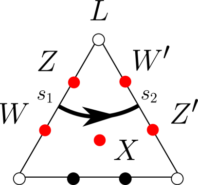
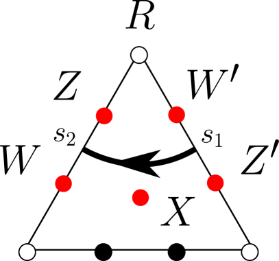
Fix an ideal triangulation of . Form the corresponding split ideal triangulation of by ‘splitting’ each edge of into a biangle . (Compare [BW11, §5].) See Figure 23. For notational simplicity, we identify the triangles of with the triangles of . A framed link is said to be in good position with respect to the split ideal triangulation if:
-
•
the link is transverse to for each edge of ;
-
•
for each triangle of , the intersection consists of a disjoint union of arcs , each connecting distinct sides of ;
-
•
the arcs are ‘flat’, in the sense that each arc has a constant height with respect to the vertical coordinate of and has the blackboard framing.
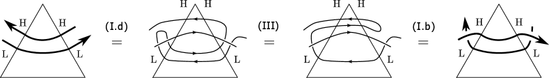
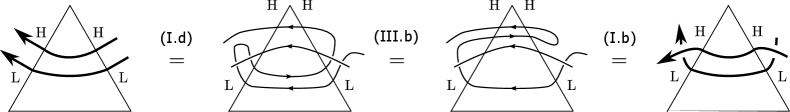
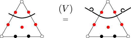
(Compare [BW11, Lemma 23].) In particular, when in good position, all of the ‘complexity’ of the link resides in the thickened biangles . A good position move between framed oriented links and in good position is one of the oriented versions of the local moves depicted in Figures 15-19 in [BW11, §5]. In the present article, these moves are displayed in Figures 24, 25, 26, 27 (Move I); Figures 28, 29 (Move II); Figures 30, 31, 32, 33 (Move III); Figures 34, 35, 36, 37 (Move IV); and, Figure 38 (Move V).
The proof of the following fact is the same as the proof of the corresponding un-oriented version ([BW11, Lemma 24]).
Fact 34.
Any framed oriented link has a good position with respect to the split ideal triangulation . Any two isotopic framed oriented links and in good position are related by a sequence of good position moves and their inverses (and isotopies through framed oriented links in good position). ∎
5.3.3. General case
Let be any blackboard-framed oriented link (recall that a framed link can be isotoped to have the blackboard framing by possibly introducing kinks). By §5.3.2, we may assume that is in good position with respect to the split ideal triangulation . Let the biangles of be denoted for and let the triangles be denoted for . Put and . By definition of good position, where each component is a flat oriented arc connecting distinct sides of . Choose indices such that lies below with respect to the height order of . For any state on , by §5.3.1, the triangle quantum torus elements are defined for . Assign such a quantum torus element to the stated link by
Note, importantly, the order in which the non-commuting elements are multiplied, the convention being ‘ordered lower to higher, multiply left to right’. For any state on , let the numbers be defined by Proposition 30.
Definition 35.
Let be a stated blackboard-framed oriented link in in good position with respect to the split ideal triangulation . The -quantum trace polynomial is defined by
where the compatibility condition (Definition 21) for the states and with respect to the state and the split triangulation is analogous to that in §5.2.4. (Compare [BW11, §6, p. 1600-1601].) Note that the quantities commute in the tensor product, since they lie in different tensor factors .
This completes the construction of the -quantum trace map for links. One would still need to show it is well-defined, that is, independent of the choice of good position (equivalently, independent of isotopy); see §6 for a proof in the case .
5.4. Properties
Assuming isotopy invariance, we conclude this section with a few observations.
The above state sum definition of the quantum trace polynomial takes as input a stated framed oriented link and outputs an element of the tensor product . We had indicated earlier (Theorem 22) that the image should lie in the Fock–Goncharov quantum torus sub-algebra ; see §3.6. The following fact is justified by a straightforward analysis of the structure of the local U-turn, crossing, left, and right matrices. (Compare [BW11, Lemma 25]. See also [Kim20], where a stronger property is established.)
Fact 36.
The quantum trace polynomial is an element of . ∎
Proof of (the general version of) Complement 23.
The Classical Trace Property is by construction, comparing with the classical matrices of §2. The State Sum Property is immediate from the construction (assuming isotopy invariance). The Multiplication Property follows from the State Sum Property by the corresponding property for biangles (Proposition 30), together with the definitions of good position and the quantities . (Compare [BW11, §6, p.1609].) ∎
We remark that the quantum trace of a stated framed oriented link can be thought of as a tensor having dimension equal to the number of boundary points of the link, each associated to a state . If the states are partitioned into two groups and , then the quantum trace of the link can be written as a matrix with coefficients in ; see §6 for examples.
5.4.1. Skein relations
We justify parts (B)-(C) in (the general version of) Theorem 22.
The first skein relation is the well-known (-evaluated) HOMFLYPT relation from knot theory [FYH+85, PT87]. The -matrices for the quantum group satisfy this skein relation. For us, this relation appears with the normalization displayed in Figure 1. One can check from, say, Figures 19(a), 19(b), 21 together with the definitions of §5.2.2 and §5.2.3 that the quantum trace map satisfies this skein relation, translating to the matrix equation
The second skein relation, coming from the U-turn ‘duality’ matrices (Figures 17 and 18), says that the contractible untwisted unknot evaluates to times the quantum integer ; see Figure 2. The third skein relation consists of the positive and negative framing relations; see Figure 3.
6. Isotopy invariance: proof of the main theorem
Proof of Theorem 22.
Parts (B)-(C) were discussed above. In this section, we will establish part (A): the -quantum trace map is invariant under isotopy. It suffices to check the oriented good position moves; see §5.3.2. We do this ‘by hand’, using computer assistance. ∎
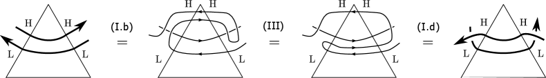
The more difficult moves are those of type (II) and (IV). Indeed, (I) can be computed directly from the definitions (although it is still somewhat non-trivial), (III) is essentially equivalent to Theorem 16, and (V) is equivalent to the kink-removing skein relations appearing in Figure 3. However, below we will justify moves (I), (III), and (V) as well.
Remark 37.
In the general case of , a proof of essentially these same algebraic identities (including Theorem 16), which are equivalent to the local isotopy moves discussed in this section, is given in [CS23] (motivated by [SS19, SS17] and earlier by [FG06a, GSV09]) in the context of quantum integrable systems; see also [GS19]. Consequently, these works can be applied to finish the proof of the general version of Theorem 22.
6.1. Notation
Throughout this section, we will be considering a single triangle with 7 coordinates, denoted as in Figure 28. (Note that the coordinates we are currently labeling as , , , , were labeled, respectively, , , , , in §5.3.1.) We define matrices and in by the same formulas as in §5.3.1. These matrices are considered as functions of the ordered -tuple . For example, we may also consider a matrix corresponding to the right turn in Figure 28.
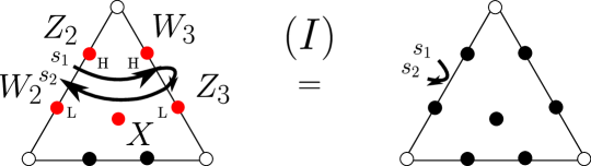
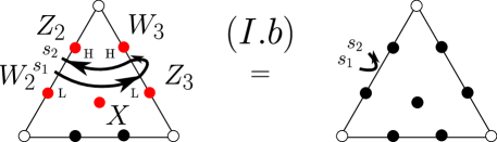
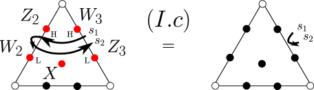
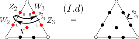
6.2. Move (I)
In Figure 24, we show one of the oriented versions of Move (I). Let be the link on the left, and the link on the right. According to the definition of the quantum trace (§5.3) as a State Sum Formula, the equality expressing Move (I) can be interpreted as an equality of matrices. Specifically, the claim is that the matrix,
| () | |||
is equal to the matrix
where we have used Figure 17(a) and the matrix from §5.2.1 for the middle matrix, and where we have put (§6.1)
See Appendix B for a computer check of the above equality of matrices in representing this oriented Move (I) example. Also checked in Appendix B are the other three oriented versions of Move (I), whose equivalent matrix formulations are displayed in Figures 25, 26, 27. (Note that the reversal of order of the non-commuting variables in the case of Moves (I) and (I.c) is due to the ‘ordered lower to higher, multiply left to right’ rule; see §5.3.)
| () | |||
| () | |||
| () | |||
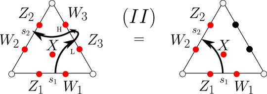
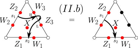
6.3. Move (II)
In Figure 28, we show one of the oriented versions of Move (II). Let be the link on the left, and the link on the right. According to the definition of the quantum trace (§5.3) as a State Sum Formula, the equality expressing Move (II) can be interpreted as an equality of matrices. Specifically, the claim is that the matrix,
| () | |||
is equal to the matrix
where we have used Figure 18(a) and the matrix from §5.2.1 for the middle matrix, and where we have put (§6.1)
See Appendix B for a computer check of the above equality of matrices in representing this oriented Move (II) example. Also checked in Appendix B is the other oriented version of Move (II), whose equivalent matrix formulation is displayed in Figure 29.
| () | |||
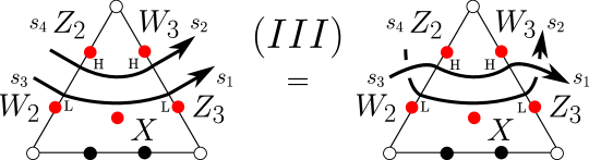
6.4. Move (III)
In Figure 30, we show one of the oriented versions of Move (III). Let be the link on the left, and the link on the right. According to the definition of the quantum trace (§5.3) as a State Sum Formula, the equality expressing Move (III) can be interpreted as an equality of matrices (§5.1). Specifically, the claim is that the matrix,
| () |
is equal to the matrix
where we have used Figures 19(b), 19(a) and the matrices and , respectively, from §5.2.2 as part of the computation for the matrix on the right, and where we have put (§6.1)
See Appendix B for a computer check of the above equality of matrices in representing this oriented Move (III) example. In Figures 31, 32, and 33 we prove the remaining oriented versions of Move (III), in terms of the moves already established.
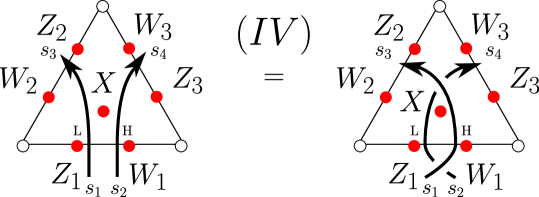
6.5. Move (IV)
In Figure 34, we show one of the oriented versions of Move (IV). Let be the link on the left, and the link on the right. According to the definition of the quantum trace (§5.3) as a State Sum Formula, the equality expressing Move (IV) can be interpreted as an equality of matrices (§5.1). Specifically, the claim is that the matrix,
| () |
is equal to the matrix
where we have used Figure 19(c) and the matrix from §5.2.2 as part of the computation for the matrix on the right, and where we have put (§6.1)
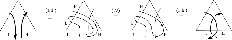
See Appendix B for a computer check of the above equality of matrices in representing this oriented Move (IV) example. In Figures 35, 36, and 37 we prove the remaining oriented versions of Move (IV). (Note that Move (I.b′) and Move (I.d′), used here, are proved in §6.7.)

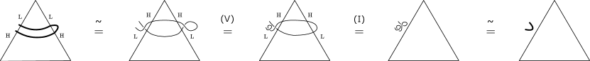
6.6. Move (V)
See Figure 38. This move is implied by the kink-removing skein relations appearing in Figure 3; see §5.4.1.
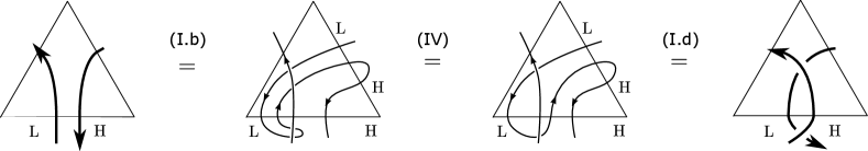
6.7. Auxiliary moves
Move (I.b′) and Move (I.d′) were used to establish Moves (IV.c) and (IV.d). The proof of Move (I.b′) is shown in Figure 39. Here denotes an isotopy preserving good position. (See also the second to last paragraph of the proof of Lemma 24 in [BW11].) The proof of Move (I.d′) is obtained from that of Move (I.b′) by horizontal reflection.
Appendix A Proof of Proposition 30
This is an application of Theorem XIV.5.1 in [Kas95]. We will closely follow the definitions, notations, and conventions of [Kas95], informing otherwise. Essentially all of the following theory is standard. See, for instance, [Kas95, BG02, JS91, Maj95].
Our first goal is to define the ribbon category of interest. In particular, this requires defining the objects , morphisms , tensor products , tensor unit , braiding morphisms (see Remark 38), dual objects , left duality morphisms and , twist morphisms , and right duality morphisms and . As above, fix , , as well as and in . This section does not require a choice of square root ; compare §5.2. All vector spaces are over .
A.1. Quantum special linear group
The quantum matrix algebra is the quotient of the free algebra in generators by the relations
for and (we think of lower indices indicating rows and upper indices columns). The quantum determinant is (compare §3.4)
The quantum special linear group is the quotient
The algebra is a Hopf algebra, meaning it is equipped with linear maps
namely the product, unit, coproduct, counit, and antipode. Specifically, if denotes the Kronecker delta (equals if and else), then the coproduct , counit , and antipode are defined by (abusing notation by using the same symbol for elements of as their images in )
where the quantum minor is the quantum determinant of the subalgebra, isomorphic to , of generated by the with and . (We write simply and .)
A.2. Braided tensor category - of right -comodules
A.2.1. Right -comodules
A vector space is a right -comodule if it is equipped with a linear map , namely a (right) coaction, satisfying certain properties. The tensor product of two right -comodules is a right -comodule, with coaction
Here, we have used Sweedler’s notation for the coactions and . The trivial right -comodule has coaction .
Let - denote the tensor category whose objects are right -comodules, morphisms are homomorphisms of right -comodules, and with tensor products and tensor unit as above.
A.2.2. Braidings
The bialgebra is cobraided, meaning it is equipped with linear maps and its inverse (with respect to the convolution operator defined in §A.3.2) , namely the universal -forms. Specifically, if is the linear map , then
Consequently, the tensor category - of right -comodules is braided, with braiding morphisms and inverse braidings (so, ) defined by
Remark 38.
By symmetry, one can just as well take the inverse braidings to be ‘the’ braidings for the category. For technical reasons, we will prefer this choice going forward. (Note that, in order to compute with , the formulas,
can be helpful, here using Sweedler’s notation for the coproduct .)
A.3. Ribbon sub-category - of finite-dimensional right -comodules
A.3.1. Left dualities
Let be a right -comodule of dimension . The dual space is a right -comodule as follows. Choose a basis for with corresponding dual basis for . Let for satisfy
The coaction is defined by
Let - denote the braided sub-category of - consisting of finite-dimensional right -comodules. Then - has left duality, the dual objects being defined as above, and with left duality morphisms and defined by
Here, is a fixed complex duality parameter.
A.3.2. Twists
The following has been adapted to our purposes from [Kas95, Chapter XIV, Exercises 5-6].
The convolution operator on the dual space is defined by
This operation makes into an algebra, with multiplicative unit the counit for . Similarly, operates on by
The cobraided Hopf algebra is coribbon, meaning there exists an invertible central element in such that
Here, is the swapping map . Specifically, and its convolution inverse are defined by
Consequently, the braided category with left duality - of finite-dimensional right -comodules (with braidings , see Remark 38) is ribbon, with twist morphisms defined by
A.3.3. Right dualities
Moreover, the ribbon category - of finite-dimensional right -comodules (with braidings , see Remark 38) has right duality, with right duality morphisms and defined by
A.4. Ribbon sub-category of - coming from the quantum row-space
A.4.1. Quantum row-space
The quantum row-space is the quotient of the free algebra in generators by the relations for . The (infinite-dimensional) algebra is a right -comodule (in fact, a right -comodule-algebra), with coaction defined by
For each integer , let denote the (finite-dimensional) sub-space of consisting of homogeneous polynomials of degree . Then is a right -sub-comodule of . For the remainder of this appendix, define by
Let denote the ribbon sub-category of - generated by . In particular, objects of are finite tensor products of and its dual .
A.4.2. Morphism formulas
We will give explicit formulas for the braidings (see Remark 38), left dualities , , twists , and right dualities , . Since we are working in the sub-category , it suffices to compute the formulas for and .
It can be shown that the braidings , , and are calculated by the same formulas as those provided in §5.2.2; see also Remark 29. The left dualities and are calculated by the formulas in §A.3.1, taking the symmetric duality parameter ; see Remark 39 and Lemma 41. The twists and can be computed by the formulas in §A.3.2 as
The right dualities and can be computed by the formulas in §A.3.3 as
A.4.3. Matrix formulas
We will make an observation for the duality morphisms similar to Fact 27. This will require our choice of the symmetric duality parameter ; see Remark 39.
Recall the matrix from §5.2.1. (See §5.1 for matrix conventions.) More generally, define for any scalar a matrix in by
Note that the matrices agree for . Similarly, define , , , and for any scalar to be the dualities defined in §A.3.1 and A.3.3 (see also §A.4.2). Recall from §5.2.2 the ordered bases and of and . When written in terms of the basis (and the basis of ), the left duality becomes a matrix with coefficients . Similarly, when written in terms of these bases, the dualities , , and become , , and matrices with coefficients , , and .
Lemma 41 (defining property of the symmetric duality parameter ).
The following equalities of matrix coefficients,
hold if and only if , where .
Proof.
We display the case of . The other computations are similar. Put . We calculate
as well as
where we define . We gather
Remark 42.
Compare the four analogous matrix equations in §5.2.1; see Figures 17 and 18. We will see the reason for the transposition of the indices , in the first two equalities of Lemma 41 when we discuss diagrammatics below. Essentially, this is because the tails of the U-turns in Figure 17, corresponding (see §A.5 and A.6) to the morphisms and , are associated with the second tensor factor (measured from bottom to top). The opposite is true for the U-turns in Figure 18, corresponding to the morphisms and .
The sign ambiguity in Lemma 41 is resolved by our need for the matrix . Why, in §5.2.1, was the matrix preferred over ? For instance, this was required for the quantum trace to satisfy the local isotopy Move (II); see Figure 28 and Equation (). (Assuming we ask for the local monodromy matrices to have positive entries.)
A.5. Category of ribbons and the Reshetikhin–Turaev functor
A.5.1. Category of ribbons
The universal ribbon category , also called the category of oriented ribbons, is defined exactly as in [Kas95, §XIV.5.1]. Roughly speaking, the objects are collections of oriented ribbon ends, and the morphisms are isotopy classes of oriented ribbons matching this end data. It is useful to, rather, think of ribbons as framed links, the link being the spine of the ribbon, and where the framing at a point on the link is normal to the tangent space of the ribbon at that point (in this way of thinking about the framing we differ from [Kas95], but it is immaterial mathematically, so long as we work with framed links rather than ribbons).
Ribbons live in the space having the usual ,,-coordinates. However, when drawing ribbon diagrams (which are, importantly, different from our previous pictures such as those appearing in Figures 17-21), the -coordinate is drawn on the page horizontally right, the -coordinate on the page vertically up, and the -coordinate into the page. By definition, the ribbon ends lying on the same boundary plane in are required to have distinct -coordinates (and isotopy preserves this property). The coordinates are called ribbon coordinates.
Ribbon diagrams always represent ribbons with the blackboard framing, meaning the constant framing in the direction, that is, out of the page toward the eye of the reader. Such a framing is always possible by introducing kinks into the ribbon. Here, a positive kink (Figure 3(a)) replaces a full right-handed twist, and a negative kink (Figure 3(b)) a full left-handed twist [Kas95, §X.8]. Note that ribbon ends lying on are also required to have this blackboard framing.
A.5.2. Reshetikhin–Turaev functor
We will apply Theorem XIV.5.1 in [Kas95]. This says that there is a unique functor from the category of ribbons to the ribbon category , which preserves the braiding, duality, and twist, and satisfies the property that a single downward-pointing (namely, negative direction) ribbon end (a distinguished object in ) is mapped to . (Consequently, upward-pointing ribbon ends are mapped to .) In particular, provides an isotopy invariant of stated oriented ribbons (see below).
Diagrammatically speaking, we use exactly the same conventions for displaying morphisms in the category as in [Kas95, Chapter XIV]. For example, in Figure 40 we show how the twist morphisms are displayed diagrammatically [Kas95, Chapters X.8 and XIV.5.1]; compare Figures 3(a)-3(b), as well as our calculations in §A.4.2. To help distinguish these ribbon diagrams from our previous pictures, as in Figures 17-21, we put a white arrow on the boundary axis indicating the positive -direction.
A.6. Alternative definition of the biangle quantum trace map
We will prove part (A) of Proposition 30. The strategy is to use the Reshetikhin–Turaev functor to give an alternative definition of the quantum trace map for a biangle , equivalent to the definition provided in §5.2. To do this, we need to be able to pass back and forth between the more symmetric topological setting of framed links in the thickened biangle (which comes without any preferred parametrization–see the beginning of §5.2), and the less symmetric categorical setting of framed links in (where the parametrization matters–see, for example, Figure 40).
A.6.1. ‘Turning your head’
To pass between the two settings, we ‘turn our head’. That is, instead of viewing the thickened biangle ‘from the top’ (as in Figures 17-21), instead we view it ‘from the side’. This can be done in two different ways, illustrated in Figure 41 (intuitively, from the perspective of Person G or that of Person D).
More precisely, let the thickened biangle have biangle coordinates with respect to a choice of parametrization (intuitively, this choice is only to tell Person G and Person D where to stand, but the point is that where they stand does not matter, as they will see the same answer). For example, in the left hand side of Figure 41, the -coordinate is drawn on the page horizontally right, the -coordinate on the page vertically up, and the -coordinate out of the page toward the eye of the reader. Then, by Figure 41 and our discussion of ribbon coordinates in §A.5.1, if , , denote the ribbon coordinates from Person G’s perspective, the G-(ribbon) coordinate transformation is
Similarly, the D-(ribbon) coordinate transformation is
Note that from either perspective the positive -ribbon coordinate corresponds to the direction of increasing height in the thickened biangle .
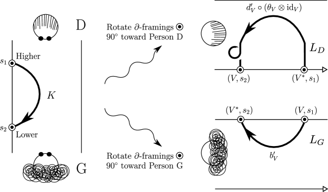
A.6.2. Definition via the Reshetikhin–Turaev functor: topological setup
Fix a stated framed oriented link in the thickened biangle ; see §4.2. Recall that by definition the framing on the boundary points up in the vertical direction. That is, the framing vector is in biangle coordinates (§A.6.1); see the left hand side of Figure 41 where the ‘bullseyes’, indicating the tips of the framing vectors, point out of the page toward the eye of the reader. Recall that, by definition, elements of lying on the same boundary component of have distinct heights, namely, distinct Z-coordinates (Remark 20).
We now ‘turn our head’ as in §A.6.1, say from the perspective of Person G. More precisely, by applying the -coordinate transformation we obtain a link in . However, is not yet a framed link, according to the definition in §A.5.1. Indeed, its framing vectors on the boundary are all in ribbon coordinates. To fix this, we rotate each framing vector 90 degrees toward Person G, yielding an appropriate framing vector We call the resulting framed link again . Similarly, by this process we obtain a, possibly different, framed link in from Person D’s perspective; see Figure 41. We say that the new framed links and have been corrected.
Importantly, note that this process of correcting the framing may introduce a twist in the link. Indeed, as an example, on the right hand side of Figure 41 the framed link acquires a right-handed twist from Person D’s perspective. On the other hand, there is no twist from Person G’s perspective.
Note also that the distinct Z-coordinates condition for the link boundary is consistent with the distinct -coordinates condition for and (see §A.5.1).
A.6.3. Definition via the Reshetikhin–Turaev functor: algebraic setup
From Person G’s perspective, let for denote the number of points of the corrected framed link lying on the boundary plane . The framed link comes with a pair of sequences of vector spaces , where the sequence is ordered in the increasing -direction; see §A.5.2. In other words, the sequences come from evaluating the Reshetikhin–Turaev functor on the domain and codomain objects of the framed link viewed as a morphism in the category of ribbons ; see §A.5.1. Moreover, the evaluation of the functor on the framed link provides a linear map
Similarly, define for , sequences of vector spaces, and a linear map from Person D’s perspective.
For example, on the right hand side of Figure 41 we see and, as a degenerate case, . The corresponding linear map is (see [Kas95, p.351]). On the other hand, from Person D’s perspective, and and the corresponding linear map is (compare Figure 40).
Let be the basis vector . By abuse of notation, we also let denote the covector . Note that provides an ordered basis for either or . From Person G’s perspective, say, we may then consider the basis for the tensor product defined by
ordered as in §5.1. Similarly, from Person D’s perspective, we define a basis for the tensor product . Note that this procedure recovers the familiar bases , , , and for , , , and used in §A.4.3 and §5.2.2.
A.6.4. Alternative definition of the -biangle quantum trace map via the Reshetikhin–Turaev functor
Recall that the framed link in the thickened biangle has in addition been equipped with a state , meaning that to each point of the boundary is associated a state-number in . From Person G’s perspective, say, mimicking the sequences we obtain a pair of sequences of state-numbers for . Similarly, from Person D’s perspective, we obtain a pair of state sequences . Note and .
For example, on the right hand side of Figure 41 we see and from Person G’s perspective. We also see and from Person D’s perspective. (Here and in Figure 41, the names of the states were arbitrary, taken from §5.2.1, and not intended to be ordered in any particular way.)
Definition 43.
Choose one of the two parametrizations of the thickened biangle , as in §A.6.1. Given a stated framed oriented link in the thickened biangle , from Person G’s perspective (Figure 41) define the complex number , depending on the parametrization , by
where denotes the matrix of the linear map written in the bases and , and with the state-numbers and . In addition, define the number (also depending on )
from Person D’s perspective (also Figure 41), where denotes the matrix of written in the bases and , and with the states and .
A.6.5. Finishing the proof of Proposition 30
Lemma 44 (symmetry of the -biangle quantum trace map).
For a given parametrization of , we have for any stated framed oriented link .
Proof.
As a first case, consider the stated link displayed in Figure 41 (and Figure 17(a)). In §A.6.3, we saw that and . By Lemma 41 and the formula for the twist appearing in §A.4.2, we compute
and
as desired. (Recall the topological discussion surrounding Figure 41, where it is important that we have chosen the symmetric duality parameter .) The proof when the stated link is one of the three other kinds of U-turns (see Figures 17(b) and 18) is similar (two of these U-turns acquire left-handed twists in ).
Next, consider the stated link displayed in Figure 19(a). Note that no twists are introduced when either or are corrected, because their constituent arcs connect different boundary components of the thickened biangle. We compute
see [Kas95, p.341], Remark 38, and Fact 27, as well as
see [Kas95, p.348] and Fact 27. The proofs for as in Figures 19(b), 19(c), and 19(d) are similar. For the other type of crossing, say, the stated link displayed in Figure 20(a), we compute in the same way
The proofs for as in Figures 20(b), 20(c), and 20(d) are similar, as well as for the trivial strand (possibly with twists), Figure 21.
The argument for a general stated link follows from the previous special cases, together with the fact that the Reshetikhin–Turaev functor satisfies the State Sum Property (essentially by definition) and is an isotopy invariant. Put into a bridge position (§5.2.4) with respect to a partition in biangle-coordinates, call the resulting link . This determines bridge-positions for and with respect to partitions and in - and -coordinates. Let and be the corresponding restricted stated links in and , where for the moment the states and are chosen arbitrarily on the internal boundaries and for . Note that each component of or is either a U-turn, crossing, or trivial strand (possibly with twists) (we are abusing the word ‘component’ here, since we are considering a crossing to be a single component). Also, upon correction of and , no components of any acquire twists, while all U-turn components (and no others) of the acquire twists, which are right-handed (resp. left-handed) when the U-turn component of has boundary with -coordinate (resp. ), namely, is a cap (resp. cup). By the coordinate transformation , , , the link is related to the link as follows: (1) as un-oriented links, they are the same, except cups (resp. caps) of the former flip to become caps (resp. cups) of the latter (with twists as described just above); (2) the orientations of U-turns, thought of as pointing along the positive or negative -direction, are preserved; (3) the orientations of same (resp. opposite) direction crossings are flipped (resp. preserved); and, (4) the orientations of trivial strands are flipped. Write (as in §A.6.4, note and ), and the restriction of these states to a component of , and similarly for Person D. If it happens that and , then by the previous special cases we have
Since and (§A.6.4), it follows by the State Sum Formula that
Lastly, by isotopy invariance,
Proof of Proposition 30.
Appendix B Computer calculations
In the Mathematica code appearing at the end of this article: section 2.1 verifies the claims for the local example of §3.5.2; section 2.2 verifies the claims for the local example of §3.5.1; section 3.2.1 verifies the claims for Moves (I), (I.b), (I.c), (I.d) of §6.2; section 3.2.2 verifies the claims for Moves (II), (II.b) of §6.3; section 3.2.3 verifies the claims for Move (III) of §6.4; and, section 3.2.4 verifies the claims for Move (IV) of §6.5.
References
- [AK17] D. G. L. Allegretti and H. K. Kim. A duality map for quantum cluster varieties from surfaces. Adv. Math., 306:1164–1208, 2017.
- [All19] D. G. L. Allegretti. Categorified canonical bases and framed BPS states. Selecta Math. (N.S.), 25:paper no. 69, 50 pp., 2019.
- [BFKB99] D. Bullock, C. Frohman, and J. Kania-Bartoszyńska. Understanding the Kauffman bracket skein module. J. Knot Theory Ramifications, 8:265–277, 1999.
- [BG93] I. Biswas and K. Guruprasad. Principal bundles on open surfaces and invariant functions on Lie groups. Internat. J. Math., 4:535–544, 1993.
- [BG02] K. A. Brown and K. R. Goodearl. Lectures on algebraic quantum groups. Birkhäuser Verlag, Basel, 2002.
- [BHMV95] C. Blanchet, N. Habegger, G. Masbaum, and P. Vogel. Topological quantum field theories derived from the Kauffman bracket. Topology, 34:883–927, 1995.
- [Bon96] F. Bonahon. Shearing hyperbolic surfaces, bending pleated surfaces and Thurston’s symplectic form. Ann. Fac. Sci. Toulouse Math. (6), 5:233–297, 1996.
- [BW11] F. Bonahon and H. Wong. Quantum traces for representations of surface groups in . Geom. Topol., 15:1569–1615, 2011.
- [BW16] F. Bonahon and H. Wong. Representations of the Kauffman bracket skein algebra I: invariants and miraculous cancellations. Invent. Math., 204:195–243, 2016.
- [CF99] L. O. Chekhov and V. V. Fock. A quantum Teichmüller space. Theoret. and Math. Phys., 120:1245–1259, 1999.
- [CF00] L. O. Chekhov and V. V. Fock. Observables in 3D gravity and geodesic algebras. Czechoslovak J. Phys., 50:1201–1208, 2000.
- [CKKO20] S. Y. Cho, H. Kim, H. K. Kim, and D. Oh. Laurent positivity of quantized canonical bases for quantum cluster varieties from surfaces. Comm. Math. Phys., 373:655–705, 2020.
- [CKM14] S. Cautis, J. Kamnitzer, and S. Morrison. Webs and quantum skew Howe duality. Math. Ann., 360:351–390, 2014.
- [CL22] F. Costantino and T. T. Q. Lê. Stated skein algebras of surfaces. J. Eur. Math. Soc. (JEMS), 24:4063–4142, 2022.
- [CS23] L. O. Chekhov and M. Shapiro. Log-canonical coordinates for symplectic groupoid and cluster algebras. Int. Math. Res. Not. IMRN, 9565-9652, 2023.
- [CTT20] A. Casella, D. Tate, and S. Tillmann. Moduli spaces of real projective structures on surfaces. Mathematical Society of Japan, Tokyo, 2020.
- [Dou20] D. C. Douglas. Classical and quantum traces coming from and . PhD thesis, University of Southern California, 2020.
- [Dou21] D. C. Douglas. Points of quantum coming from quantum snakes, to appear in Algebr. Geom. Topol. https://arxiv.org/abs/2103.04471, 2021.
- [DS20] D. C. Douglas and Z. Sun. Tropical Fock-Goncharov coordinates for -webs on surfaces II: naturality. https://arxiv.org/abs/2012.14202, 2020.
- [DS24] D. C. Douglas and Z. Sun. Tropical Fock-Goncharov coordinates for -webs on surfaces I: construction. Forum Math. Sigma, 12:paper no. e5, 55 pp., 2024.
- [FG06a] V. V. Fock and A. B. Goncharov. Cluster -varieties, amalgamation, and Poisson-Lie groups. In Algebraic geometry and number theory, volume 253 of Progr. Math., pages 27–68. Birkhäuser Boston, Boston, MA, 2006.
- [FG06b] V. V. Fock and A. B. Goncharov. Moduli spaces of local systems and higher Teichmüller theory. Publ. Math. Inst. Hautes Études Sci., 103:1–211, 2006.
- [FG07a] V. V. Fock and A. B. Goncharov. Dual Teichmüller and lamination spaces. Handbook of Teichmüller theory, 1:647–684, 2007.
- [FG07b] V. V. Fock and A. B. Goncharov. Moduli spaces of convex projective structures on surfaces. Adv. Math., 208:249–273, 2007.
- [FG09] V. V. Fock and A. B. Goncharov. Cluster ensembles, quantization and the dilogarithm. Ann. Sci. Éc. Norm. Supér., 42:865–930, 2009.
- [FKBL19] C. Frohman, J. Kania-Bartoszyńska, and T. T. Q. Lê. Unicity for representations of the Kauffman bracket skein algebra. Invent. Math., 215:609–650, 2019.
- [Foc97] V. V. Fock. Dual Teichmüller spaces. https://arxiv.org/abs/dg-ga/9702018, 1997.
- [FS22] C. Frohman and A. S. Sikora. -skein algebras and webs on surfaces. Math. Z., 300:33–56, 2022.
- [FWZ16] S. Fomin, L. Williams, and A. Zelevinsky. Introduction to cluster algebras. Chapters 1-3. https://arxiv.org/abs/1608.05735, 2016.
- [FYH+85] P. Freyd, D. Yetter, J. Hoste, W. B. R. Lickorish, K. Millett, and A. Ocneanu. A new polynomial invariant of knots and links. Bull. Amer. Math. Soc. (N.S.), 12:239–246, 1985.
- [FZ02] S. Fomin and A. Zelevinsky. Cluster algebras. I. Foundations. J. Amer. Math. Soc., 15:497–529, 2002.
- [Gab17] M. Gabella. Quantum holonomies from spectral networks and framed BPS states. Comm. Math. Phys., 351:563–598, 2017.
- [GMN14] D. Gaiotto, G. W. Moore, and A. Neitzke. Spectral networks and snakes. Ann. Henri Poincaré, 15:61–141, 2014.
- [Gol84] W. M. Goldman. The symplectic nature of fundamental groups of surfaces. Adv. Math., 54:200–225, 1984.
- [Gol86] W. M. Goldman. Invariant functions on Lie groups and Hamiltonian flows of surface group representations. Invent. Math., 85:263–302, 1986.
- [GS19] A. B. Goncharov and L. Shen. Quantum geometry of moduli spaces of local systems and representation theory. https://arxiv.org/abs/1904.10491, 2019.
- [GSV09] M. Gekhtman, M. Shapiro, and A. Vainshtein. Poisson geometry of directed networks in a disk. Selecta Math. (N.S.), 15:61–103, 2009.
- [Hig23] V. Higgins. Triangular decomposition of skein algebras. Quantum Topol., 14:1–63, 2023.
- [Hit92] N. J. Hitchin. Lie groups and Teichmüller space. Topology, 31:449–473, 1992.
- [HN16] L. Hollands and A. Neitzke. Spectral networks and Fenchel-Nielsen coordinates. Lett. Math. Phys., 106:811–877, 2016.
- [IY23] T. Ishibashi and W. Yuasa. Skein and cluster algebras of unpunctured surfaces for . Math. Z., 303:paper no. 72, 60 pp., 2023.
- [JS91] A. Joyal and R. Street. An introduction to Tannaka duality and quantum groups. In Category theory (Como, 1990), volume 1488 of Lecture Notes in Math., pages 413–492. Springer, Berlin, 1991.
- [Kas95] C. Kassel. Quantum groups. Springer-Verlag, New York, 1995.
- [Kas98] R. M. Kashaev. Quantization of Teichmüller spaces and the quantum dilogarithm. Lett. Math. Phys., 43:105–115, 1998.
- [Kim20] H. K. Kim. -laminations as bases for cluster varieties for surfaces, to appear in Mem. Amer. Math. Soc. https://arxiv.org/abs/2011.14765, 2020.
- [Kim21] H. K. Kim. Naturality of quantum trace maps for surfaces. https://arxiv.org/abs/2104.06286, 2021.
- [KLS23] H. K. Kim, T. T. Q. Lê, and M. Son. quantum trace in quantum Teichmüller theory via writhe. Algebr. Geom. Topol., 23:339–418, 2023.
- [Kup96] G. Kuperberg. Spiders for rank 2 Lie algebras. Comm. Math. Phys., 180:109–151, 1996.
- [Lab06] F. Labourie. Anosov flows, surface groups and curves in projective space. Invent. Math., 165:51–114, 2006.
- [Lê18] T. T. Q. Lê. Triangular decomposition of skein algebras. Quantum Topol., 9:591–632, 2018.
- [LS21] T. T. Q. Lê and A. S. Sikora. Stated -skein modules and algebras. https://arxiv.org/abs/2201.00045, 2021.
- [LY23] T. T. Q. Lê and T. Yu. Quantum traces for -skein algebras. https://arxiv.org/abs/2303.08082, 2023.
- [Maj95] S. Majid. Foundations of quantum group theory. Cambridge University Press, Cambridge, 1995.
- [MFK94] D. Mumford, J. Fogarty, and F. Kirwan. Geometric invariant theory. Third edition. Springer-Verlag, Berlin, 1994.
- [NY20] A. Neitzke and F. Yan. -nonabelianization for line defects. J. High Energy Phys., paper no. 153, 65 pp., 2020.
- [NY22] A. Neitzke and F. Yan. The quantum UV-IR map for line defects in -type class theories. J. High Energy Phys., paper no. 81, 50 pp., 2022.
- [Pro76] C. Procesi. The invariant theory of matrices. Adv. Math., 19:306–381, 1976.
- [Prz91] J. H. Przytycki. Skein modules of 3-manifolds. Bull. Polish Acad. Sci. Math., 39:91–100, 1991.
- [PT87] J. H. Przytycki and P. Traczyk. Conway algebras and skein equivalence of links. Proc. Amer. Math. Soc., 100:744–748, 1987.
- [RT90] N. Y. Reshetikhin and V. G. Turaev. Ribbon graphs and their invariants derived from quantum groups. Comm. Math. Phys., 127:1–26, 1990.
- [Sik01] A. S. Sikora. -character varieties as spaces of graphs. Trans. Amer. Math. Soc., 353:2773–2804, 2001.
- [Sik05] A. S. Sikora. Skein theory for -quantum invariants. Algebr. Geom. Topol., 5:865–897, 2005.
- [SS17] G. Schrader and A. Shapiro. Continuous tensor categories from quantum groups I: algebraic aspects. https://arxiv.org/abs/1708.08107, 2017.
- [SS19] G. Schrader and A. Shapiro. A cluster realization of from quantum character varieties. Invent. Math., 216:799–846, 2019.
- [Thu97] W. P. Thurston. Three-dimensional geometry and topology. Vol. 1. Princeton University Press, Princeton, NJ, 1997.
- [Thu14] D. P. Thurston. Positive basis for surface skein algebras. Proc. Natl. Acad. Sci. USA, 111:9725–9732, 2014.
- [Tur89] V. G. Turaev. Algebras of loops on surfaces, algebras of knots, and quantization. In Braid group, knot theory and statistical mechanics, volume 9 of Adv. Ser. Math. Phys., pages 59–95. World Sci. Publ., Teaneck, NJ, 1989.
- [Wit89] E. Witten. Quantum field theory and the Jones polynomial. Comm. Math. Phys., 121:351–399, 1989.
See pages - of appendix-NEWEST