Quantum thermodynamics as a gauge theory

Let us consider a quantum system associated with the Hilbert space $\mathcal{H}^{d}$, whose dimension is denoted as $\dim\{\mathcal{H}^{d}\}=d$. To construct the thermodynamic group, we assume the following: (i) $\mathcal{H}^{d}$ is finite-dimensional; (ii) the thermodynamic quantities are functionals of the density matrix; (iii) the gauge transformations are unitary.

The first assumption is not overly restrictive since $d$ can be as large as we please. It is important to remember that most experiments involve a limited number of particles, typically under well-defined boundary conditions. Therefore, we usually deal with systems that effectively have a countable number of energy eigenstates. Even for a continuous degree of freedom, detectors have finite resolution, which introduces coarse-graining into the system, thus allowing for a description in terms of finite, countable energy states. The second assumption asserts that every physical quantity must be a functional of the density operator, which contains the information about the system. While it can also be a function of other operators, such as the Hamiltonian, it will always be a function of the density matrix. The third assumption is based on the fact that every continuous symmetry group, which is the case here, admits a unitary representation. We will revisit this point at the end of the paper.

These assumptions alone are not sufficient to define the thermodynamic group. Considering all possible unitary transformations would render the theory trivial and not useful [28]. Therefore, we must impose a physical restriction on this set. Since we are discussing Thermodynamics and symmetry transformations, it is natural to require that the action of the gauge group should not change the mean energy of the system

with $H_{t}$ and $\rho$ being the (possibly time-dependent) system Hamiltonian and density matrix, respectively. From this, we define the following principle

Using this definition, we can explicitly construct the thermodynamic group [28]. First, note that energy invariance under $V_{t}$ implies that $[V_{t},H_{t}]=[V^{\dagger}_{t},H_{t}]=0$, since this must hold for any density operator. Therefore, the gauge transformations $V_{t}$ are unitary channels that commute with the Hamiltonian. It is important to emphasise that $V_{t}$ is not equivalent to the thermal operations defined in the context of the resource theory of thermodynamics [30, 31]. Instead, the thermodynamic gauge forms a very particular subclass of these transformations, which are not associated with any physical interpretation. For more details, see Ref. [28].

The construction of the symmetry group proceeds as follows. Since the Hamiltonian is hermitian, it can be written as

where $p$ is the number of distinct energy eigenvalues $\lambda^{k}_{t}$, while $n_{t}^{k}$ stands for the multiplicity of each $\lambda^{k}_{t}$, at each instant of time $t$. That is, $n_{t}^{k}$ is the instantaneous degree of degeneracy of the $k$-th energy eigenvalue. We must have $\sum_{k=1}^{p}n_{t}^{k}=d$. $\mathbb{1}_{a}$ is the identity matrix with dimension $a$. Note that $n_{t}^{k}$ is allowed to change in time. This will have very important physical consequences.

Given the Hamiltonian decomposition in Eq. (3), along with the condition $[H_{t},V_{t}]=0$, all $V_{t}$ must be of the form

where $v^{k}_{t}\in\mathcal{U}(n_{t}^{k})$, the set of unitary matrices of dimension $n_{t}^{k}$. From the perspective of group representation theory, $\mathcal{V}_{t}$ is decomposed in unitary irreducible representations $v_{t}^{k}$ of each $\mathcal{U}(n_{t}^{k})$. Importantly, this is associated to the decomposition of the Hilbert space $\mathcal{H}^{d}=\bigoplus_{k=1}^{p}\mathcal{H}_{k}$ where each $\mathcal{H}_{k}$ is the subspace spanned by the eigenvectors associated to the $k$-th eigenvalue.

Furthermore, Eq. (4) provides another characterisation to the thermodynamic group. In fact, $[V_{t},H_{t}]\leavevmode\nobreak\ =\leavevmode\nobreak\ 0\leavevmode\nobreak\ \iff\leavevmode\nobreak\ [\mathcal{V}_{t},h_{t}]\leavevmode\nobreak\ =\leavevmode\nobreak\ 0$ and we can describe the gauge transformation using both $V_{t}$ or $\mathcal{V}_{t}$. Therefore, regarding Definition 1, $\mathcal{V}_{t}$ preserves the mean energy with respect to diagonal Hamiltonian $h_{t}$.

Now, from Eq. (4) we can formally define

The topological aspects of the thermodynamic group can be analysed by introducing the isomorphic group $\mathcal{G}_{\operatorname{T}}$, with is associated to each matrix $\mathcal{V}_{t}$ in Eq. (4).

Given such an isomorphism, from now on we refer to $\mathcal{G}_{\operatorname{T}}$ as the thermodynamic group.

The group $\mathcal{G}_{\operatorname{T}}$ is directly associated with each matrix $v^{k}_{t}$ in Eq. (4) and the subgroups $\mathcal{U}(n_{t}^{k})$ of $\mathcal{U}(d)$, this is a schematic representation in Fig. 1. From the topological point of view, the thermodynamic group is constructed from a product of finite compact Lie subgroups. $\mathcal{G}_{\operatorname{T}}$ is therefore, also a compact Lie group, whose Lie algebra $\mathfrak{g}_{\operatorname{T}}$ fulfills the relation $\dim\{\mathfrak{g}_{\operatorname{T}}\}\leq\dim\{\mathfrak{u}(d)\}$, which follows from Eq. (6) as a consequence of degeneracy.

In this context, consider that if a given eigenvalue $\lambda^{m}_{t}$ is non-degenerate, the corresponding matrix $v^{m}_{t}$ satisfies $v^{m}_{t}\in\mathcal{U}(1)$. Consequently, $v^{m}_{t}$ contributes to the matrix $\mathcal{V}_{t}$ with only one arbitrary element, namely $(\mathcal{V}_{t})_{mm}$, while all other elements associated with this block vanish, i.e., $(\mathcal{V}_{t})_{mj}=(\mathcal{V}_{t})_{jm}=0$ for $j\neq m$. In contrast, if any energy eigenvalue is degenerate, the associated matrix $v^{k}_{t}$ is not necessarily diagonal. In fact, the most general form of $v^{k}_{t}$ is a unitary matrix of order $n_{t}^{k}\times n_{t}^{k}$, i.e. $v^{k}_{t}\in\mathcal{U}(n_{t}^{k})$, with all elements non-zero.

Therefore, each non-degenerate eigenvalue contributes to the dimension of the Lie algebra of the thermodynamic group with a basis associated with the Lie algebra of the group $\mathcal{U}(n_{t}^{k}=1)$, whose dimension is $1$. On the other hand, degenerate eigenvalues contribute to the dimension of the Lie algebra with $\mathcal{U}(n_{t}^{k}>1)$, whose dimension is $(n_{t}^{k})^{2}$.

It is interesting to consider two illustrative situations. The first case, explored in Ref. [28], corresponds to a fully non-degenerate energy spectrum, i.e. $n_{t}^{k}=1$ for all $k$. In this case, $\mathcal{V}_{t}$ is diagonal, since $\left[\mathcal{V}_{t},h_{t}\right]=0$ and $h_{t}$ are diagonal with distinct elements. Therefore, the dimension of the Lie algebra associated with $\mathcal{G}_{\operatorname{T}}$ is $\dim\{\mathfrak{g}_{\operatorname{T}}\}=d$, and the group is a $d$-fold tensor product of trivial phases which are elements of $\mathcal{U}(1)$. The second interesting case involves a Hamiltonian with a fully degenerate spectrum. In this case, the gauge group is $\mathcal{G}_{\operatorname{T}}=\mathcal{U}(d)$, and the dimension of the associated Lie algebra is $d^{2}$. The group is a $d^{2}$-fold tensor product of elements belonging to $\mathcal{U}(d)$.

Now that we have the structure of the thermodynamic group, we can use the gauge invariance principle to construct all the quantities physically relevant in our theory. Such quantities are those that remain invariant under the action of $\mathcal{G}_{\operatorname{T}}$.

As previously noted, all physical quantities relevant to thermodynamics are represented as functionals of the system’s density matrix, $\rho_{t}$. Specifically, we often focus on a particular set of physical quantities, such as energy, heat, and work.

The application of Definition 3 to the usual notions of work [Eq. (12)] and heat [Eq. (13)] provided the notions of work and heat which are invariant with respect to the thermodynamic group [28]. These are the physical work and heat we refer in the present framework.

As a final important comment on the hypothesis in 1, the results in Eqs. (14) and (15) are established under the condition that the unitary matrix $u_{t}$ is differentiable for all $t$. This condition ensures that the expressions for invariant work and heat do not change even if degeneracies vary over time. However, it is possible to develop an associated process when $u_{t}$ is not continuous. A particularly relevant physical case is the quench process, where the Hamiltonian suddenly changes at a given time. Quench dynamics is used to study a variety of physically interesting phenomena in the context of many-body physics, such as chaos [37], Anderson localisation [38], many-body localisation [39, 40], and thermodynamic aspects of quantum phase transitions (QPTs) [41, 42, 43, 44]. Following this, in the next section, we will study the invariant work and heat for quench processes and apply this to QPTs. However, before this, let us see how the thermodynamic entropy emerges from our framework.

Remembering that our theory is built on the basis of Quantum Information Theory, it is natural to consider Von Neumann entropy as the measure of information, from which the invariant thermodynamic entropy emerges through Eq. (9). Formally, we established the in the following.

The $\mathcal{G}_{\operatorname{T}}-$entropy is the von Neumann entropy for the average of the density matrix with respect to the thermodynamic group. This entropy is deeply connected with two quantum physical features: degeneracies and coherences. The connection with degeneracies is obvious, as it emerges from the definition of the thermodynamic group in Eq. (6) and the invariant quantities in Eq. (9). On the other hand, the connection with coherences can be established by the relationship between $\mathcal{G}_{\operatorname{T}}-$entropy and the diagonal entropy, $S_{d}[\rho(t)]=S_{u}[\rho_{diag}]$, where $\rho_{diag}$ is the density operator with the off-diagonal elements (in the energy eigenbasis) removed.

We introduce $S_{\Gamma}[f_{t}]$ and $f_{t}$ just to simplify notation. In fact, $f_{t}$ is not a density matrix, and $S_{\Gamma}$ is not the von Neumann entropy. The relation in Eq. (20), however, is highly helpful for studying the properties of $\mathcal{G}_{\operatorname{T}}-$entropy. Notably, $S_{\Gamma}[f_{t}]$ represents the difference between the contributions obtained by the Haar average and the usual contributions from the populations in the diagonal entropy. Specifically, if the energy spectrum is non-degenerate, the blocks of $f_{t}$ coincide, leading to $S_{\Gamma}=0$. Consequently, the $\mathcal{G}_{\operatorname{T}}$-entropy reduces to the diagonal entropy. On the other hand, when the energy spectrum is completely degenerate, the first block of $f_{t}$ coincides with the diagonal density matrix in energy eigenbasis, and the relation in Eq. (20) reduces to $S_{\mathcal{G}_{\operatorname{T}}}$ in Eq. (18).

The expression for $f_{t}$ in Eq. (20) is non-trivial as long as there is at least one non-degenerate energy level. However, even if the energy spectrum is completely degenerate, Eq. (20) is always valid, since $S_{\mathcal{G}_{\operatorname{T}}}\geq S_{diag}$, thus implying that $S_{\Gamma}\geq 0$. In this sense, we identify that the term $S_{\Gamma}$ precisely corresponds to the Holevo asymmetry measure [34, 47] associated with the diagonal part of the density operator in the energy basis.

Moreover, we can prove that the equality in $S_{\mathcal{G}_{\operatorname{T}}}=S_{diag}$ is achieved if and only if the energy spectrum is non-degenerate. Consequently, the diagonal entropy naturally emerges from the $\mathcal{G}_{\operatorname{T}}$-entropy. From the point of view of the Holevo asymmetry measure, this implies that the states are completely symmetric [34] with respect to the thermodynamic group $\mathcal{G}_{\operatorname{T}}$.

Therefore, the relation between diagonal entropy and $S_{\mathcal{G}_{\operatorname{T}}}$ suggests interpreting $S_{\mathcal{G}_{\operatorname{T}}}$ as a generalised measure of the amount of randomness observed in the energy eigenbasis of both degenerate and non-degenerate systems. In this way, the Holevo asymmetry measure $S_{\Gamma}$ is associated with the amount of randomness introduced into the system due to degenerate energy levels, a pure quantum feature. Furthermore, we can see the similarity between the contributions of coherent heat in Eq. (27) and $\mathcal{G}_{\operatorname{T}}-$entropy. We have contributions associated with coherences and degeneracies, indicating a relationship between coherent heat and $\mathcal{G}_{\operatorname{T}}-$entropy. The proofs of all these results are proved in Appendix B.

In order to gain deeper insights into the physical aspects of our theory, we next apply it to two paradigmatic examples in many-body physics: the Landau-Zener and the Lipkin-Meshkov-Glick models.

Let us consider the dynamics of a single qubit described by the following Hamiltonian

where $\sigma^{x}$ and $\sigma^{z}$ are Pauli matrices, and $g$ stands for the strength of the externally controlled magnetic field, whose coupling with the qubit is represented by $a>0$. $\epsilon$ is associated with the crossing ($\epsilon=0$) or non-crossing ($\epsilon>0$) energy levels and $\Delta$ is the bare frequency of the qubit.

Hamiltonian Eq. (29) is the well-known Landau-Zener model, which is frequently employed in studies of phase transitions as it is a prototype for critical systems [51, 41]. The system undergoes a quantum phase transition at the critical point $g_{c}=\Delta/2a$ and $\epsilon\to 0$. For $\epsilon>0$, the transition is a first-order one, characterised by a discontinuous change in the order parameter. When $\epsilon=0$, the transition becomes a second-order one, exhibiting a continuous change in the order parameter and associated critical fluctuations. A schematic representation of these situations is presented in Fig. 3.

Figure 4 reveals the behaviour of the work [panel 4(a)], heat [panel 4(b)], and entropy [panel 4(c)] for distinct quenches from $g_{0}$ to $g=g_{0}+\delta g$. In particular, panel 4(a) shows that the invariant work exhibits a similar behaviour to that observed for the derivative of the ground state energy of the model, as shown in Fig.3. This similarity is especially pronounced in the regime of small quenches, i.e., $\delta g\to 0$. Furthermore, for small quenches, panel 4(b) indicates that the coherent heat approaches zero, suggesting a negligible contribution of energy associated with the change of basis during the quench. Indeed, for $Q_{c}[\rho]\approx 0$ and considering the system with no degeneracies, we can connect $W_{\text{inv}}[\rho]$ with the variation of the ground state energy with respect to the parameter $g_{0}$ as

which follows from the Hellman-Feynman Theorem [52]. The expression in Eq. (33) justifies the correspondence between the variation of the ground state energy and the invariant work in Figs. 3 and 4(a).

Another interesting aspect to consider in the Landau-Zener model is the case with energy level crossing, i.e., $\epsilon=0$. In this case, the contribution of heat is zero, which is expected since $[H_{0},H_{\tau}]=0$. However, the model exhibits degeneracy at the critical point $g_{0}=\Delta/4a$. At this point, the thermodynamic group $\mathcal{G}_{\operatorname{T}}$ is isomorphic to the group $\mathcal{U}(2)$. Consequently, the Haar measure induced by the thermodynamic group is $\differential\mathcal{G}_{\operatorname{T}}^{g_{c}}=\differential\mu\left[\mathcal{U}(2)\right]$. Therefore, it follows that the expression for the invariant work is modified to $W_{\text{inv}}[\rho]=-a\delta g/2\operatorname{sgn}\left(g_{0}-\Delta/2\right)$, where $\operatorname{sgn}(\cdot)$ denotes the sign function.

Signatures of the QPT can be seen in the derivatives of invariant work and heat. As the system approaches the critical point of the phase transition, these quantities exhibit divergent behaviour. This divergence is visually evident in Fig. 5. These expressions are all obtained in Appendix C.

Let us now consider a more complex system, exhibiting degenerate eigenlevels and quantum phase transition, described by the Hamiltonian

where $J_{\alpha}=\sum_{i=1}^{N}\sigma^{\alpha}_{i}/2;$ $(\alpha=x,y,z)$ are the collective spin operators, with $\sigma_{i}^{\alpha}$ denoting the $\alpha$ Pauli matrix acting on the $i$-th site of a chain of $N=2j$ sites, and $j$ is the total angular momentum. The parameters $k>0$, $0\leq\gamma\leq 1$, and $g\geq 0$ denote the constants associated with the coupling between the spins, the anisotropy of the model, and the strength of the magnetic field along the $x$-axis, respectively.

The Hamiltonian in Eq. (34) is a particular instance of the well-known Lipkin-Meshkov-Glick model [53, 54, 55]. Various properties of the LMG model have already been studied in the literature in different contexts such as nuclear physics [56], optics [57], quantum information [58], and condensed matter [59], just to mention a few. Therefore, given its wide applicability, it is the right model for us to consider its quantum thermodynamics in the context of gauge invariance.

In the thermodynamic limit, i.e., $j\to\infty$, the model presents a quantum phase transition [49, 42] where the parity symmetry is broken as the magnetic field changes from $g<g_{c}$ (ferromagnetic phase) to $g>g_{c}$ (paramagnetic phase), where $g_{c}=k$ is the critical point of the equilibrium phase transition [42]. A particular feature of these two phases is related to degeneracies of the Hamiltonian. While the ferromagnetic phase is doubly degenerated, the paramagnetic phase presents no degeneracy. Figure. 6 shows such configurations.

Given this feature, the invariant work, heat and entropy does not reduce to the simple form that we saw in the Landau-Zener model. The average of the density matrix over the thermodynamic group assumes the general form given in Eq. (11). In order to apply our theory to the case in hand, we consider the time dependent counterpart associated to the Hamiltonian Eq. (34) as

A direct consequence of the theory emerges from the expression for the invariant work. It is an order parameter for the system, since the magnetisation $\langle J_{\alpha}\rangle=\operatorname{Tr}\{\rho J_{\alpha}\}$ (with $\alpha=x,y,z$) is the usual order parameter signalling the quantum phase transition in the this case [41]. We show such behaviour in Fig. 7(a), where the order parameter feature of the work is clear. The other panels in this figure show the dynamical behaviour of the first and second derivatives of the work with respect to the quench parameter $g_{0}$. While the second derivative diverges near the critical point, the first derivative exhibits oscillations, which are a consequence of the changes in the degeneracies as we change $g_{0}$. It is clear from these figures that the invariant work is deeply linked to the quantum phase transition.

Another interesting result that follows form the theory is associated to the invariant heat, which is shown in Fig. 8. We can see that the heat suffers and abrupt change near the critical point of the model, while the divergence of its derivative with respect to the quench clearly signs this point.

Now we discuss the thermodynamic entropy $S_{\mathcal{G}_{\operatorname{T}}}$ for the case at hand, which is not equivalent to the diagonal entropy as in the Landau-Zener model, since we have degeneracies. As mentioned earlier, the ferromagnetic phase ($g<g_{c}$) is doubly degenerate, while the paramagnetic phase ($g>g_{c}$) is completely non-degenerate. Therefore, we expect very distinct behaviours of $S_{\mathcal{G}_{\operatorname{T}}}$ in both phases. This is shown in Fig. 9.

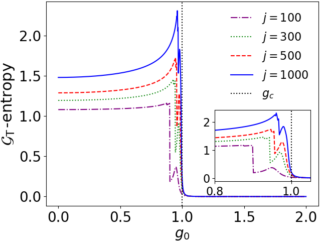
We first observe the similarity between the $\mathcal{G}_{\operatorname{T}}$-entropy in Fig. 9 and the heat displayed in Fig. 8(a). This fact is not a coincidence but a consequence of the theory that makes both quantities directly associated with the production of quantum coherence in the energy eigenbasis, as well as with the presence of degeneracies in the ferromagnetic phase. In particular, this result confirms and extends the understanding of heat proposed in Ref. [28].

Moreover, Fig. 9 clearly shows a tendency for an abrupt change in $S_{\mathcal{G}_{\operatorname{T}}}$ in the vicinity of the critical point. Such change occurs precisely at the point where the degeneracies of the system are completely extinguished due to the competition between the contributions of the spin coupling and the external magnetic field. The extinction of degeneracies before the critical point occurs because we are dealing with a finite-dimensional system.

However, as shown in the Fig. 9, this point tends to shift to the critical point of the model for larger dimensions, where we approach the thermodynamic limit. Additionally, we observe that the abrupt change in $S_{\mathcal{G}_{\operatorname{T}}}$ is more pronounced in chains with fewer spins, which is associated with the contributions of degeneracies being more significant in systems further away from the thermodynamic limit.

Accordingly, we analyze $S_{\mathcal{G}_{\operatorname{T}}}$ in comparison with the diagonal entropy $S_{d}$, highlighting the contributions of degeneracies as quantified by the Holevo asymmetry measure $S_{\Gamma}$ and also the effect of the size of the chain. First, we observe from Fig. 10 that oscillatory behavior of the Holevo asymmetry measure in the vicinity of the critical point arises from the breaking of energy level degeneracies, which results in modifications to the structure of the thermodynamic group $\mathcal{G}_{\operatorname{T}}$. As the value of $j$ increases, the oscillations in the Holevo asymmetry $S_{\Gamma}$ decrease near the critical point and eventually vanish at the quantum phase transition.

Then, from the point of view of the Holevo asymmetry measure, degeneracies produce asymmetry and consequently increase the randomness and entropy of the state. However, it is the relationship between the total volume of the subspaces $\mathcal{H}_{k}$ and the changes in degeneracies that leads to abrupt modifications in the thermodynamic entropy. Consequently, we expect a greater impact of degeneracies in lower-dimensional systems, since the Haar averages contained in $S_{\Gamma}$ are significant with respect to the contributions of populations coming from the diagonal entropy.

Thus, for large values of $j$, near the critical point of the phase transition, the diagonal entropy approaches $S_{\mathcal{G}_{\operatorname{T}}}$, while the Holevo asymmetry fluctuates around values close to zero. Indeed, this behaviour emerges because the contributions of the remaining degeneracies are not as significant as in smaller dimensions, as shown by the $S_{\Gamma}$ curve in Figs. 10 and 11. Therefore, from Eq. (20) it follows that near the critical point $|S_{\mathcal{G}_{\operatorname{T}}}-S_{d}|=S_{\Gamma}$ and, since $S_{\Gamma}$ becomes increasingly less significant, we conclude that the $\mathcal{G}_{\operatorname{T}}$-entropy and the diagonal entropy approach each other. Thus, the Holevo asymmetry acts as a parameter that determines the continuity of the thermodynamic gauge entropy.

On the other hand, for quenches occurring after the critical point of the phase transition, we observe that $S_{\mathcal{G}_{\operatorname{T}}}$ asymptotically tends to zero. Indeed, after the critical point, the thermodynamic group is always given by $\mathcal{G}_{\operatorname{T}}=\prod_{k=1}^{d}\mathcal{U}(1)$, and consequently, the diagonal part of the states $\rho$ in the energy basis becomes increasingly symmetric with respect to the group $\mathcal{G}_{\operatorname{T}}$, thereby asymptotically reducing the entropy.

References

- [1] John Goold, Marcus Huber, Arnau Riera, Lídia del Rio, and Paul Skrzypczyk. “The role of quantum information in thermodynamics — a topical review”. J. Phys. A: Math. Theor. 49, 143001 (2016).
- [2] Herbert B. Callen. “Thermodynamics and an introduction to thermostatistics”. Student Edition. Wiley India Pvt. Limited. (2006). url: https://books.google.com.br/books?id=uOiZB_2y5pIC.
- [3] Francis A Di Bella. “Applying engineering thermodynamics: A case study approach”. World Scientific. (2021).
- [4] Eduardo Mizraji. “Homeostasis and information processing: The key frames for the thermodynamics of biological systems”. Biosyst. 236, 105115 (2024).
- [5] E. Deli, J. Peters, and Z. Kisvárday. “The thermodynamics of cognition: A mathematical treatment”. Comput. Struct. Biotechnol. J. 19, 784 (2021).
- [6] Dieter H E Gross. “Microcanonical thermodynamics: Phase transitions in "small" systems”. World Scientific. (2001).
- [7] Charles H. Bennett. “The thermodynamics of computation — a review”. Int. J. Theor. Phys. 21, 905–940 (1982).
- [8] Robert M. Wald. “The thermodynamics of black holes.”. Living Rev. in Rel.4 (2001).
- [9] Philipp Strasberg. “Quantum stochastic thermodynamics: Foundations and selected applications”. Oxford University Press. (2022).
- [10] Elliott H. Lieb and Jakob Yngvason. “The physics and mathematics of the second law of thermodynamics”. Phys. Rep. 310, 1–96 (1999).
- [11] Robin Giles. “Mathematical foundations of thermodynamics”. Pergamon. (1964).
- [12] Robert Alicki. “The quantum open system as a model of the heat engine”. J. Phys. A: Math. Gen. 12, L103 (1979).
- [13] Robert Alicki and Ronnie Kosloff. “Introduction to quantum thermodynamics: History and prospects” (2018). arXiv:1801.08314.
- [14] Felix Binder, Luis A. Correa, Christian Gogolin, Janet Anders, and Gerardo Adesso, editors. “Thermodynamics in the quantum regime: Fundamental aspects and new directions”. Springer International Publishing. Cham (2018).
- [15] Jorge Kurchan. “A quantum fluctuation theorem” (2001). arXiv:0007360.
- [16] Peter Talkner, Eric Lutz, and Peter Hänggi. “Fluctuation theorems: Work is not an observable”. Phys. Rev. E 75, 050102 (2007).
- [17] Jordan M Horowitz and Juan M R Parrondo. “Entropy production along nonequilibrium quantum jump trajectories”. New J. Phys. 15, 085028 (2013).
- [18] Matteo Lostaglio, David Jennings, and Terry Rudolph. “Description of quantum coherence in thermodynamic processes requires constraints beyond free energy”. Nat. Commun. 6, 6383 (2015).
- [19] Peter Talkner and Peter Hänggi. “Aspects of quantum work”. Phys. Rev. E 93, 022131 (2016).
- [20] John von Neumann. “Thermodynamik quantenmechanischer gesamtheiten”. Nachrichten von der Gesellschaft der Wissenschaften zu Göttingen, Mathematisch-Physikalische Klasse 1927, 273–291 (1927). url: http://eudml.org/doc/59231.
- [21] Anatoli Polkovnikov. “Microscopic diagonal entropy and its connection to basic thermodynamic relations”. Ann. Phys. 326, 486–499 (2011).
- [22] R. Kawai, J. M. R. Parrondo, and C. Van den Broeck. “Dissipation: The phase-space perspective”. Phys. Rev. Lett. 98, 080602 (2007).
- [23] Takahiro Sagawa. “Second law-like inequalities with quantum relative entropy: An introduction”. Pages 125–190. World Scientific Pub. (2012).
- [24] Vlatko Vedral. “The role of relative entropy in quantum information theory”. Rev. Mod. Phys. 74, 197–234 (2002).
- [25] Gabriel T. Landi and Mauro Paternostro. “Irreversible entropy production: From classical to quantum”. Rev. Mod. Phys. 93, 035008 (2021).
- [26] Steven Weinberg. “The quantum theory of fields, vol. 1: Foundations”. Cambridge University Press. (2005).
- [27] Carlo Rovelli. “Quantum gravity”. Cambridge Monographs on Mathematical Physics. Univ. Pr. Cambridge, UK (2004).
- [28] Lucas C. Céleri and Łukasz Rudnicki. “Gauge-invariant quantum thermodynamics: Consequences for the first law”. Entropy 26, 111 (2024).
- [29] R Medeiros de Araújo, T Häffner, R Bernardi, D S Tasca, M P J Lavery, M J Padgett, A Kanaan, L C Céleri, and P H Souto Ribeiro. “Experimental study of quantum thermodynamics using optical vortices”. J. Phys. Commun. 2, 035012 (2018).
- [30] Fernando G. S. L. Brandão, Michał Horodecki, Jonathan Oppenheim, Joseph M. Renes, and Robert W. Spekkens. “Resource theory of quantum states out of thermal equilibrium”. Phys. Rev. Lett. 111, 250404 (2013).
- [31] Eric Chitambar and Gilad Gour. “Quantum resource theories”. Rev. Mod. Phys. 91, 025001 (2019).
- [32] William Fulton and Joe Harris. “Representation theory: A first course”. Graduate Texts in Mathematics. Springer New York. (1991).
- [33] Antonio Anna Mele. “Introduction to Haar Measure Tools in Quantum Information: A Beginner’s Tutorial”. Quantum 8, 1340 (2024).
- [34] Stephen D. Bartlett and H. M. Wiseman. “Entanglement constrained by superselection rules”. Phys. Rev. Lett. 91, 097903 (2003).
- [35] Christoph Dankert, Richard Cleve, Joseph Emerson, and Etera Livine. “Exact and approximate unitary 2-designs and their application to fidelity estimation”. Phys. Rev. A 80, 012304 (2009).
- [36] M.A. Nielsen and I.L. Chuang. “Quantum computation and quantum information: 10th anniversary edition”. Cambridge University Press. (2010).
- [37] Karthik Chinni, Pablo M. Poggi, and Ivan H. Deutsch. “Effect of chaos on the simulation of quantum critical phenomena in analog quantum simulators”. Phys. Rev. Res. 3, 033145 (2021).
- [38] Stefano Marcantoni, Federico Carollo, Filippo M. Gambetta, Igor Lesanovsky, Ulrich Schneider, and Juan P. Garrahan. “Anderson and many-body localization in the presence of spatially correlated classical noise”. Phys. Rev. B 106, 134211 (2022).
- [39] Dmitry A. Abanin, Wojciech De Roeck, and François Huveneers. “Theory of many-body localization in periodically driven systems”. Ann. Phys. 372, 1–11 (2016).
- [40] Nicole Yunger Halpern, Christopher David White, Sarang Gopalakrishnan, and Gil Refael. “Quantum engine based on many-body localization”. Phys. Rev. B 99, 024203 (2019).
- [41] E. Mascarenhas, H. Bragança, R. Dorner, M. Fran ça Santos, V. Vedral, K. Modi, and J. Goold. “Work and quantum phase transitions: Quantum latency”. Phys. Rev. E 89, 062103 (2014).
- [42] Steve Campbell. “Criticality revealed through quench dynamics in the lipkin-meshkov-glick model”. Phys. Rev. B 94, 184403 (2016).
- [43] Pedro H. S. Bento, Adolfo del Campo, and Lucas C. Céleri. “Krylov complexity and dynamical phase transition in the quenched lipkin-meshkov-glick model”. Phys. Rev. B 109, 224304 (2024).
- [44] Andesson B Nascimento and Lucas C Céleri. “Quantum dynamical criticality speeds up thermodynamic entropy production” (2024). arXiv:2407.03315.
- [45] Anatoli Polkovnikov. “Microscopic expression for heat in the adiabatic basis”. Phys. Rev. Lett. 101, 220402 (2008).
- [46] Gustavo de Oliveira and Lucas Chibebe Céleri. “Thermodynamic entropy production in the dynamical casimir effect”. Phys. Rev. A 109, 012807 (2024).
- [47] Iman Marvian and Robert Spekkens. “Extending noether’s theorem by quantifying the asymmetry of quantum states”. Nat. Commun. 5, 3821 (2014).
- [48] Subir Sachdev. “Quantum phase transitions”. Cambridge University Press. (2011).
- [49] Nicolò Defenu, Alessio Lerose, and Silvia Pappalardi. “Out-of-equilibrium dynamics of quantum many-body systems with long-range interactions”. Phys. Rep. 1074, 1–92 (2024).
- [50] F. Plastina, A. Alecce, T. J. G. Apollaro, G. Falcone, G. Francica, F. Galve, N. Lo Gullo, and R. Zambrini. “Irreversible work and inner friction in quantum thermodynamic processes”. Phys. Rev. Lett. 113, 260601 (2014).
- [51] Adalberto D. Varizi, Raphael C. Drumond, and Gabriel T. Landi. “Quantum quench thermodynamics at high temperatures”. Phys. Rev. A 105, 062218 (2022).
- [52] R. P. Feynman. “Forces in molecules”. Phys. Rev. 56, 340–343 (1939).
- [53] H. J. Lipkin, N. Meshkov, and A. J. Glick. “Validity of many-body approximation methods for a solvable model: (I). Exact solutions and perturbation theory”. Nucl. Phys. 62, 188–198 (1965).
- [54] N. Meshkov, A.J. Glick, and H.J. Lipkin. “Validity of many-body approximation methods for a solvable model: (II). Linearization procedures”. Nucl. Phys. 62, 199–210 (1965).
- [55] A.J. Glick, H.J. Lipkin, and N. Meshkov. “Validity of many-body approximation methods for a solvable model: (III). Diagram summations”. Nucl. Phys. 62, 211–224 (1965).
- [56] A. M. Romero, J. Engel, Ho Lun Tang, and Sophia E. Economou. “Solving nuclear structure problems with the adaptive variational quantum algorithm”. Phys. Rev. C 105, 064317 (2022).
- [57] Gang Chen, J. Q. Liang, and Suotang Jia. “Interaction-induced lipkin-meshkov-glick model in a bose-einstein condensate inside an optical cavity”. Opt. Express. 17, 19682–19690 (2009).
- [58] Mir Afrasiar, Jaydeep Kumar Basak, Bidyut Dey, Kunal Pal, and Kuntal Pal. “Time evolution of spread complexity in quenched lipkin–meshkov–glick model”. J. Stat. Mech.: Theory Exp. 2023, 103101 (2023).
- [59] Ho-Man Kwok, Wen-Qiang Ning, Shi-Jian Gu, and Hai-Qing Lin. “Quantum criticality of the lipkin-meshkov-glick model in terms of fidelity susceptibility”. Phys. Rev. E 78, 032103 (2008).
- [60] Markus Heyl. “Dynamical quantum phase transitions: a review”. Rep. Prog. Phys. 81, 054001 (2018).
- [61] Leopoldo Nachbin and L. Bechtolsheim. “The haar integral”. University Series in Higher Mathematics : a series of advanced text and reference books in pure and applied mathematics. Princeton, N.J. : Van Nostrand. (1965). url: https://books.google.com.br/books?id=KMA-AAAAIAAJ.
- [62] Luiz A. B. San Martin. “Lie groups”. Springer Cham. (2021).
- [63] Paul R. Halmos. “Measure theory”. Graduate Texts in Mathematics. Springer New York. (2014).
- [64] Howard Barnum, M. A. Nielsen, and Benjamin Schumacher. “Information transmission through a noisy quantum channel”. Phys. Rev. A 57, 4153–4175 (1998).
- [65] Joy A. Thomas Thomas M. Cover. “Elements of information theory”. John Wiley & Sons. (2012).
- [66] Mark M. Wilde. “Quantum information theory”. Cambridge University Press. (2017).