Quantum synchronization effects induced by strong nonlinearities
Abstract
A paradigm for quantum synchronization is the quantum analog of the Stuart–Landau oscillator, which corresponds to a van der Pol oscillator in the limit of weak (i.e. vanishingly small) nonlinearity. Due to this limitation, the quantum Stuart–Landau oscillator fails to capture interesting nonlinearity-induced phenomena such as relaxation oscillations. To overcome this deficiency we propose an alternative model which approximates the Duffing–van der Pol oscillator to finitely large nonlinearities while remaining numerically tractable. This allows us to uncover interesting phenomena in the deep-quantum strongly-nonlinear regime with no classical analog, such as the persistence of amplitude death on resonance. We also report nonlinearity-induced position correlations in reactively coupled quantum oscillators. Such coupled oscillations become more and more correlated with increasing nonlinearity before reaching some maximum. Again, this behavior is absent classically. We also show how strong nonlinearity can enlarge the synchronization bandwidth in both single and coupled oscillators. This effect can be harnessed to induce mutual synchronization between two oscillators initially in amplitude death.
Introduction.—Mathematical modelling has shown us how the immense variety and beauty of nature can be governed by nonlinear differential equations May (2019); Edelstein-Keshet (2005); Jordan and Smith (2007); Debnath (2012). Such equations, owing to their nonlinearity, are difficult to analyze and their application to physical processes has come to be known as nonlinear science Campbell (1987); Scott (2006).
How nonlinear effects play out in quantum-mechanical systems is a subject of intense investigation. By far, chaos has attracted the most attention Stöckmann (2000); Haake (1991); Waltner (2012); Wimberger (2014). Nonetheless, noise effects, such as stochastic resonance Gammaitoni et al. (1998); Wellens et al. (2003); Ludwig (2019); Wagner et al. (2019) and coherence resonance Wellens et al. (2003); Kato and Nakao (2021) have also been prominent, while a recent example is Ref. Schmolke and Lutz (2023). Another widely recognized effect is noise-induced transitions Horsthemke and Lefever (2006). Recent work has extended this effect to quantum mechanics by using a quantum stochastic differential equation and its correspondence to nonlinear dissipation Chia et al. (see also Ref. Chia et al. (2020a)). There are also promising applications of nonlinear dissipation such as stabilizing bosonic qubits for fault-tolerant quantum computing Mirrahimi et al. (2014); Leghtas et al. (2015); Chamberland et al. (2022), and enhancing the sensitivity of quantum sensors Dutta and Cooper (2019); Sánchez Muñoz et al. (2021).
A relative newcomer to the study of nonlinear effects in quantum systems is synchronization Rosenblum and Pikovsky (2003). Its most elementary form consists of applying a sinusoidal force, say with amplitude , and frequency , to a self-sustained oscillator. Synchronization is then the modification of the oscillator frequency to . A prototypical model is the driven van der Pol (vdP) oscillator Strogatz (2018), defined by phase-space coordinates satisfying
| (1) |
where primes denote differentiation with respect to the argument (in this case , representing time). In the absence of forcing () the oscillator is characterized by , and a nonlinearity parameter which controls how much the oscillator is damped towards an amplitude of order . An important feature of the undriven vdP system is the existence of a supercritical Hopf bifurcation at , via which a stable limit cycle appears for Strogatz (2018).
At , (1) is entirely linear. This motivates one to consider the quasilinear limit of (1), defined by . In this limit the vdP oscillator is well approximated by the Stuart–Landau (SL) oscillator, the steady state of which is rotationally symmetric in phase space (a circular limit cycle). This makes the SL oscillator much simpler to analyze, and has thus served as a starting point in the literature on quantum synchronization for continuous-variable systems, e.g. Refs. Lee and Sadeghpour (2013); Walter et al. (2014); Sonar et al. (2018); Mok et al. (2020); Lee et al. (2014); Bastidas et al. (2015); Weiss et al. (2017); Walter et al. (2015); Morgan and Hinrichsen (2015); Ishibashi and Kanamoto (2017); Amitai et al. (2018); Bandyopadhyay et al. (2020, 2021); Kato et al. (2019); Kato and Nakao (2020); Bandyopadhyay and Banerjee (2021). The trade-off of course, is that effects taking place at finite values of are excluded. A well known example of this is relaxation oscillations in the undriven vdP oscillator111In fact, vdP intended for (1) to model relaxation oscillations in an electrical circuit Ginoux and Letellier (2012). To observe relaxation oscillations in quantum theory one needs to quantize the exact vdP model, and it is only relatively recently that such efforts have been made Shah et al. (2015); Chia et al. (2020b); Ben Arosh et al. (2021). Jordan and Smith (2007); Strogatz (2018); Jenkins (2013). More effects start to appear if driving is included, such as quasiperiodicity and chaos Broer and Takens (2011); Lakshmanan and Rajaseekar (2012); Moon (2008), both of which are absent in the driven SL oscillator.
In this work, we investigate the effects of nonlinearity in quantum oscillators by considering a more general model based on the classical Duffing–van der Pol (DvdP) oscillator. This adds to where is another nonlinearity parameter. To overcome the inadequacy of the SL model we propose a quantum DvdP oscillator in which the vdP and Duffing nonlinearities (respectively and ) are nonvanishing, but also not arbitrarily large. Our model is accurate up to order , at which the distinct signatures of strong nonlinearity appear, such as relaxation oscillations Chia et al. (2020b). Our approach has the benefit of capturing novel nonlinear effects while evading the large computational cost of simulating quantum systems with very strong nonlinear dissipations.
We show that for a single oscillator with periodic forcing there exists a critical Duffing nonlinearity, above which further increases in enlarges the synchronization bandwidth (the amount of detuning the forcing can tolerate from the oscillator and still entrain it). This result is similar to the synchronization enhancement from the classical literature Antonio et al. (2015), but now generalized to quantum oscillators.222It is also worth mentioning that nonlinear oscillators are of interest to quantum information too, when they are coupled to qubits. In this context the Duffing nonlinearity has been shown to both increase and stabilize the oscillator-qubit entanglement Montenegro et al. (2014). In contrast, the vdP nonlinearity activates genuine quantum effects. Coupling two vdP oscillators dissipatively may lead to either amplitude death (the cessation of oscillations), or mutual synchronization. Classically, amplitude death occurs only when the two oscillators are sufficiently detuned Saxena et al. (2012). Interestingly, we find this need not be the case for quantum oscillators. We show that two quantum vdP oscillators possessing relatively small limit cycles and nonvanishing nonlinearities can exhibit amplitude death even with zero detuning. Larger limit cycles on the other hand can mutually synchronize from a state of amplitude death if their nonlinearity is increased.
We also consider reactively coupled oscillators. Two such SL oscillators cannot develop positional correlations, and hence do not synchronize. This is true regardless of whether the oscillators are classical or quantum. We show here that at finitely large nonlinearity, position correlations behave rather differently between the classical and quantum oscillators: Two reactively coupled quantum vdP oscillators can undergo nonlinearity-induced correlations whereby their position correlation increases as they become more nonlinear. In contrast, we find that making the analogous classical oscillators more nonlinear monotonically reduces their position correlation. The nonlinearity-induced correlations in the quantum vdP oscillators are thus a consequence of both their quantum nature and strong nonlinearity.
Model.—For simplicity we consider here a dimensionless DvdP model in terms of the nonlinearity parameters and in which is a dimensionless scale parameter:
| (2) |
Note that is now a function of , and we have also included a dimensionless external force parameterized by and . From the approximate analysis of (2), the leading contribution to the oscillator frequency is quadratic in , and linear in (see Appendix), given by . This motivates a Bogoliubov–Krylov time-average of the equations of motion up to these orders, giving Sanders et al. (2007)
| (3) |
where . For , (3) predicts a limit-cycle amplitude of with the expected frequency shifts due to and . Additionally, note the first-order averaging in for yields the SL equation. Our approximate model captures the effects of strong vdP nonlinearity of order . We seek a quantum master equation such that (with ) agrees with (3) in the mean-field limit Chia et al. (2020b). It can then be shown that this is satisfied by the Lindbladian Lindblad (1976); Gorini et al. (1976); Breuer and Petruccione (2002)
| (4) |
where
| (5) |
We have also defined for any , and a dot denotes the position of when acted upon by a superoperator. Detailed derivation can be found in the Appendix. We remark that both the higher-order Kerr terms and the nonlinear two-photon dissipation in our proposed model can be implemented in circuit QED Hillmann and Quijandría (2022); Leghtas et al. (2015). The tunability of the limit cycle radius allows us to access different parameter regimes of the quantum oscillator, in particular the quantum (), and semiclassical () regimes. We have included the second-order contributions in in our model for its nonlinearity-tuning capability, since the terms linear in neither affect the limit-cycle amplitude nor phase dynamics. The Duffing nonlinearity translates to a Kerr term in . This model can be considered as an alternative to the quantum SL oscillator, but with flexibility in tuning the nonlinearity. All our numerical results for a given parameter set are obtained with a sufficiently large truncation of the Hilbert space by ensuring the corresponding steady-state power spectrum converge.
Nonlinearity-enhanced synchronization.—We study first the frequency locking of the approximate quantum DvdP oscillator to a periodic force [(4) and (5)]. The synchronization bandwidth is the range of for which the oscillator frequency is locked to the driving frequency at steady state. This is achieved when , where the observed frequency of the driven oscillator, obtained from the peak of its spectrum averaged over one period of the drive Chia et al. (2020b).
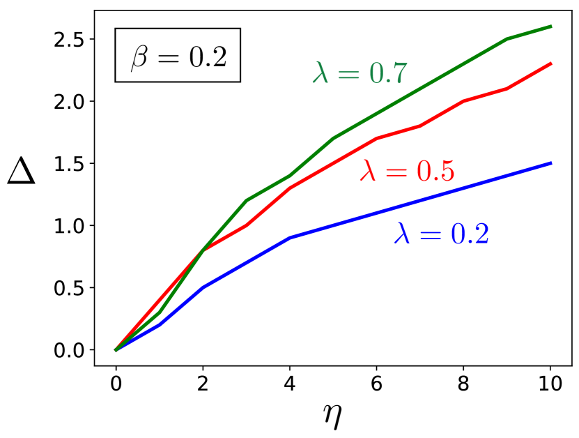
Here we find the Duffing nonlinearity to enhance quantum synchronization: For a range of and a fixed , increasing past a critical value widens the synchronization bandwidth linearly. This is illustrated in Fig. 1(a) where the synchronization bandwidth is plotted as a contour against and . The critical value of is indicated by the red dashed line, where the bandwidth is equal to its corresponding value at . However, this enhancement does not occur for all values of the vdP nonlinearity. In Fig. 1(b) we see that an increase of from its value in Fig. 1(a) can ruin the gain in synchronization bandwidth due to . Noting that the dissipative terms in are all proportional to , this effect can be qualitatively attributed to the phase diffusion due to quantum noise, which is known to inhibit synchronization Walter et al. (2014); Lee et al. (2014); Lee and Sadeghpour (2013). We can develop some understanding of the quantum DvdP by examining its classical analog. Using the method of harmonic balance on , we are able to derive the conditions for nonlinearity-enhanced synchronization analytically for the classical DvdP oscillator (see derivation in Appendix), given by
| (6) |
This shows clearly the existence of a critical value of , and a finite interval of over which the synchronization enhancement occurs. These results are consistent with Fig. 1 except for the fact that quantum noise makes the range of for synchronization enhancement in the quantum DvdP oscillator smaller compared to the classical range as seen in Fig. 1(b).
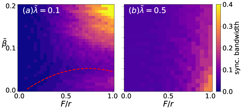
We have also shown in Appendix that increasing the vdP nonlinearity in the quantum model can only reduce the synchronization bandwidth. One can thus be certain that the synchronization enhancement seen in our model is induced by the Duffing nonlinearity. We shall see next that the vdP nonlinearity can induce synchronization in coupled oscillators from a state of amplitude death.
Nonlinearity-induced synchronization and amplitude death.—Two dissipatively coupled vdP oscillators (i.e. no Duffing nonlinearity) can be described by the Lindbladian
| (7) |
where () is the Lindbladian for oscillator , defined by setting to and in (4) and (5). We have assumed the oscillators to be identical (i.e. same and ) except for an initial detuning of , and denoted their coupling strength by .
In this case, frequency locking occurs when the observed frequencies of the two oscillators become identical at steady state. As before, the observed frequency of oscillator is given by the location at which its spectrum is peaked, i.e. where is maximized, and where the two-oscillator steady state is to be used. For a fixed , we define the synchronization bandwidth to be the range of for which the two oscillators lock frequencies. It will also be interesting to look at position correlations in the two oscillators at steady state, defined by
| (8) |
where . Note that frequency locking implies a nonzero , but not vice versa.
In addition to frequency locking, dissipatively coupled oscillators can also cease to oscillate. If the oscillators are classical, then this may happen for a range of provided that is sufficiently large. And if both oscillators stabilize to the same phase-space point, which may be taken to be the origin without loss of generality, then the effect is termed amplitude death Saxena et al. (2012); Koseska et al. (2013). To define amplitude death in quantum oscillators we generalize the notion of P-bifurcations from classical stochastic systems to the steady-state Wigner function of a reduced state (see Ref. Chia et al. and other references therein). In this case, amplitude death is said to occur if the single-oscillator Wigner functions peak at the origin in quantum phase space. This approach is consistent with previous studies on amplitude death in coupled quantum oscillators Bandyopadhyay et al. (2020); Amitai et al. (2018); Bandyopadhyay et al. (2021); Ishibashi and Kanamoto (2017).
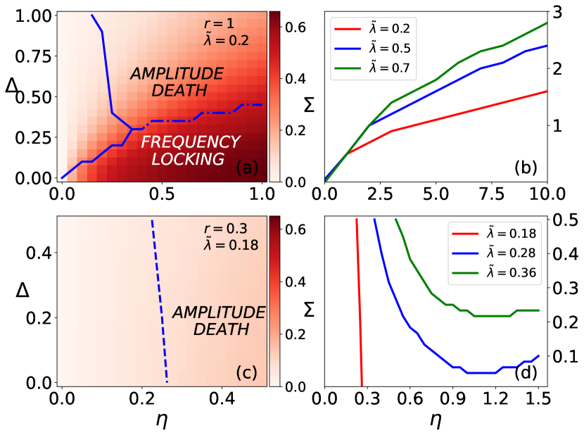
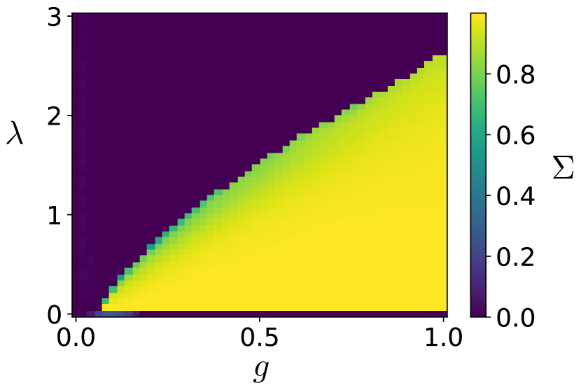
In Fig. 2 we work out regions of frequency locking and amplitude death in the parameter space for (7), along with , shown as a contour in Fig. 2(a) and (c). Two especially interesting scenarios are—when the limit cycles are relatively large compared to quantum noise [Fig. 2(a)]; and when they become small, being more susceptible to quantum noise [Fig. 2(c)].
In Fig. 2(a) we have indicated the boundary between frequency locking and amplitude death by a dash-dotted line, while no identifiable phenomenon occurs to the left of the solid line. Note the dash-dotted line is a Hopf-bifurcation curve because the transition from amplitude death to frequency locking is facilitated by a Hopf bifurcation. Clearly, is larger inside the frequency-locking region. Especially significant here is the effect of the vdP nonlinearity on synchronization. Whereas in the single-oscillator case the vdP nonlinearity had only detrimental effects, it now has a constructive role by enlarging the (mutual) synchronization bandwidth. We illustrate this in Fig. 2(b) where additional frequency-locking boundaries for different values of vdP nonlinearity are plotted. It can be seen that increasing enlarges the frequency-locking region (see also Appendix for some classical analysis). This means that two oscillators in a state of amplitude death with an lying above the Hopf-bifurcation curve in Fig. 2(a) will transit suddenly to a state of synchronized oscillations when is sufficiently increased. This may be appropriately called nonlinearity-induced mutual synchronization.
Turning now to the case of a small limit cycle in Fig. 2(c), we find frequency locking to be absent while position correlations become negligible. The blue solid line delineates the boundary of amplitude death. Most striking is the persistence of amplitude death at zero detuning (i.e. ). Classically, some frequency mismatch between the two oscillators must be present in order for amplitude death to occur Saxena et al. (2012). This signifies a clear distinction between classical and quantum dynamics. A loss of amplitude death at may then be expected if we increased either or (while holding the other constant). This is indeed what we find, as illustrated in Fig. 2(d), where such a quantum-to-semiclassical transition is captured by increasing .
Since we have focused exclusively on the vdP nonlinearity here, we note that incorporating a Duffing nonlinearity into our model will not in fact change the frequency-locking boundary. We can understand this from the classical coupled equations of motion, where we see that appears only in the phase dynamics of the oscillators, and that such terms vanish at steady state for identical oscillators (equal limit cycle radii) Aronson et al. (1990).
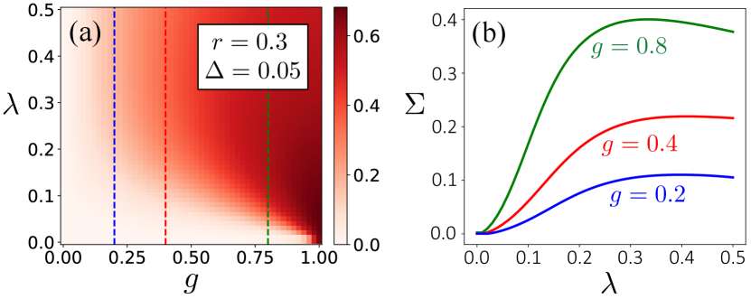
Nonlinearity-induced correlations.—It is known that two reactively coupled SL oscillators cannot synchronize nor share position correlations. This is true even in the quantum case (see Appendix). However, we show here that positional correlations between two reactively coupled quantum vdP oscillators do develop. Here we must use the exact vdP Lindbladian Chia et al. (2020b), because under reactive coupling, the approximate model does not produce any off-diagonal elements in the steady state, and hence cannot generate correlations in the two oscillators. As with the dissipatively coupled system, two reactively coupled vdP oscillators can be modelled by considering two uncoupled vdP oscillators with annihilation operators and , coupled by the Hamiltonian , where is the reactive coupling strength. As before, we assume that both oscillators have the same nonlinearity .
In Fig. 3(a), we generate a contour plot of as a function of and at and . From this we see that for a fixed , increasing the oscillator nonlinearity beyond the SL regime leads to stronger correlations. We illustrate this more clearly in Fig. 3(b) by showing how varies as a function of for , 0.4, and 0.8, which are marked in Fig. 3(a) by vertical dashed lines. Note this also shows the existence of an optimal which maximizes . Such nonlinearity-induced correlations are absent in the corresponding classical model. At a given coupling strength, the position correlation in two reactively coupled classical vdP oscillators decreases monotonically as increases (see Appendix).
Conclusion.— Our work goes beyond the well-studied paradigm of weak nonlinearity in quantum synchronization, and provides the first systematic study of quantum synchronization effects for strong nonlinearity. We introduced a new quantum oscillator model which captures intriguing effects induced by two strong nonlinearities. We showed that a strong Duffing nonlinearity leads to a linear enhancement of the synchronization bandwidth in driven oscillators. We also reported genuine quantum synchronization effects exclusive to strong nonlinearity which are not observed previously: Increasing the vdP nonlinearity enhances the synchronization bandwidth, and revives synchronization between dissipatively-coupled oscillators in amplitude death. For reactively-coupled vdP oscillators on the other hand, we find that strong nonlinearity induces position correlations which are impossible in the weakly-nonlinear limit. Our model provides a new paradigm for studying other strongly nonlinear effects such as chaos Stöckmann (2000); Strogatz (2018); Haake (2000); Braun (2001).
Acknowledgements.
Acknowledgements.—YS and WJF would like to thank the support from NRF-CRP19-2017-01. CN was supported by the National Research Foundation of Korea (NRF) grant funded by the Korea government (MSIT) (NRF-2022R1F1A1063053). WKM, AC and LCK are grateful to the National Research Foundation, Singapore and the Ministry of Education, Singapore for financial support.Appendix A Exact quantum model
Here, we describe how the quantum master equation for the exact Duffing-van der Pol model is obtained, following the approach in Chia et al. (2020b). Starting from the classical equation (2) in the main text, and defining the complex amplitude , we get the equation of motion
| (9) |
Quantum theory defines the state of a dynamical system by a density operator satisfying , where is a linear superoperator. By regarding as the analog of , where , we can quantize a system prescribed by by searching for an such that in the Schrödinger picture, . Note that we have chosen to normally order , denoted by colons [e.g. if , then ]. Such an corresponding to (9) can be found in Lindblad form Lindblad (1976); Gorini et al. (1976); Breuer and Petruccione (2002), and which we refer to as a Lindbladian:
where
| (10) |
We remark that the choice of the master equation is not unique, since we only demand that the classical equation of motion is recovered in the mean-field limit. Different choices of the master equation will in general lead to different quantum noise effects, which are most pronounced at low excitations (sometimes referred to as the deep quantum limit Mok et al. (2020)).
Appendix B A single forced classical oscillator
B.1 Poincaré–Lindstedt method
The Poincaré–Lindstedt method is a perturbative technique to find approximate periodic solutions Strogatz (2018). Regular perturbation theory fails at long time due to the existence secular terms. Taking to be the perturbative parameter, such secular terms in the van der Pol (vdP) oscillator are of the form , which are unbounded in . The Poincaré–Lindstedt method overcomes this problem by removing secular terms explicitly.
Let us consider the undriven vdP oscillator (setting ). Defining a rescaled time where is the oscillation frequency, we have the equation
| (11) |
where a prime denotes differentiation with respect to the argument. Now, we perform the perturbative expansions
| (12) | ||||
| (13) |
Collecting terms of the same order in , the zeroth-order equation reads
| (14) |
which just describes simple harmonic oscillations given by , where . The first-order equation reads
| (15) |
The resonant forcing gives rise to secular terms such as and which are unwanted. Hence, setting the resonant forcing to zero yields which gives , . This is the Stuart–Landau (SL), i.e. weakly nonlinear limit of the vdP which describes quasiharmonic oscillations. Solving the resulting first-order equation, we get the leading-order correction for : . To obtain the leading-order correction for , we look at the second-order equation
| (16) |
Again, eliminating the resonant forcing, we get . In terms of , we then have
| (17) | ||||
| (18) |
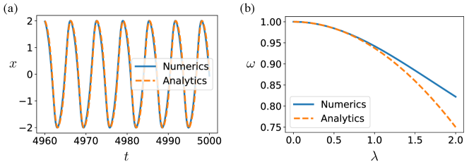
Thus, the effect of small nonlinearity on the limit cycle is a decrease in frequency and a distortion without a change in the limit cycle amplitude (from the first-order approximation of we can see that for the amplitude of the oscillation is constant at 2. Hence, the amplitude is unchanged to order .) A numerical simulation of and observed frequency as given by (18) are plotted in Fig. 4. Good agreement between the analytic and numeric simulation can be seen for .
B.2 Krylov–Bogoliubov averaging
The Krylov–Bogoliubov averaging method essentially assumes that the amplitude is slowly varying and can be treated as a constant when averaging the dynamics over one period, which produced the time-averaged equations of motion. Introducing the complex amplitude,
| (19) |
where , we can rewrite the vdP equation as a complex equation of motion
| (20) |
Performing the Krylov–Bogoliubov time averaging to first-order in , we obtain
| (21) |
which is the well-known SL equation representing the normal form of a supercritical Hopf bifurcation. The stable oscillations are described by . This gives which is consistent with the Poincaré–Lindstedt method up to zeroth order in .
The second-order averaging yields Sanders et al. (2007)
| (22) |
which predicts a limit cycle amplitude of and frequency , again consistent with the zeroth-order Poincaré–Lindstedt method.
B.3 Synchronization analysis
Here, we use the harmonic-balance method to analyze the synchronization behavior for the Duffing–van der Pol (DvdP) equation in nondimensionalized form, given by
| (23) |
Note that for ease of writing we have omitted tildes for and all dimensionless parameters (e.g. time). We then assume a synchronized solution of the form , where is the amplitude of the motion and is a constant phase shift from the driving force. Substituting the ansatz for into (23), we get
| (24) |
The second term on the left-hand side may be written as
| (25) |
Neglecting the higher harmonics and then collecting the coefficients of and , we obtain
| (26) |
These may be expressed compactly as a single complex equation as
| (27) |
| (28) |
Substituting (28) into (27) then gives the first-order equation in ,
| (29) |
The modulus of the left-hand side must be , hence we have
| (30) |
This can be solved to obtain the relationship between and . In order to derive the synchronization frequency range, we first notice that (30) is a quadratic equation in . For synchronization to exist, must be real, hence the discriminant must be non-negative, i.e.,
| (31) |
which yields
| (32) |
Hence, the vdP oscillator is synchronized if the driving frequency is within the critical interval
| (33) |
The synchronization bandwidth is thus
| (34) |
Evidently, by fixing , , and , the synchronization bandwidth becomes independent of the scale parameter . As shown in the main text, this does not hold true in the quantum case due to quantum noise. Defining
| (35) |
the bandwidth can be rewritten as
| (36) |
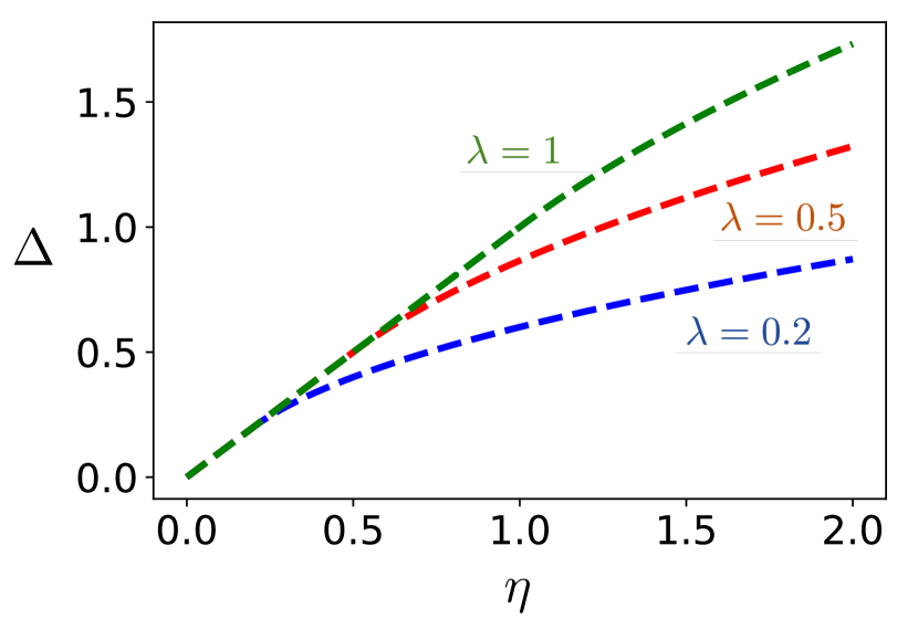
where in the last step we have taken the limit of large and small . For the usual vdP oscillator (), the synchronization bandwidth reduces to which is independent of . In order to obtain nonlinearity-induced enhancement in the bandwidth, we require
| (37) |
This results in the conditions
| (38) |
Without loss of generality, we can set in the following discussion. In this case , , and . Interestingly, the nonlinearity-induced enhancement only acts for a finite range of and requires a minimum . In the limit of large , the bandwidth tends to . However, the method of harmonic balance assumes and to be weak. In this regime, we can interpret the existence of a minimum as a competition between the effects of and . Note that the oscillator frequency is from our previous analysis. The threshold for synchronization enhancement occurs when these two opposite effects on the frequency are of the same scale, i.e. .
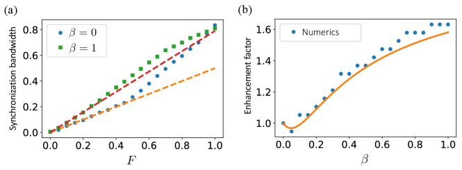
Figure 5 shows the effect of adding the Duffing nonlinearity on the synchronization bandwidth for . Comparing and in Fig. 5(a), we can see that the synchronization bandwidth is enhanced for the case for weak to moderate forcing (compared to ). The analytical prediction of the bandwidth agrees with the numerical simulations up to , beyond which the numerical bandwidth exceeds the predicted value indicating the suppression of natural dynamics at strong forcing. Using , we also predict that the synchronization enhancement occurs when . Indeed, by plotting in Fig. 5(b) the enhancement factor, defined as the ratio between the bandwidth and its baseline value , we see a good agreement between the numerical results and the analytical calculations. Fluctuations in the numerics can be attributed to a few reasons, such as the time resolution in the simulation, the number of samples used for , the frequency resolution used in determining the bandwidth, and the threshold observed detuning used to determine the frequency-locked regions (set to 0.001). The numerical results also appear to deviate slightly from the prediction at large , which is likely due to the breakdown in making the ansatz used in the derivation. Including higher harmonics in the ansatz might result in more accurate predictions at larger .
Appendix C Two classical oscillators with dissipative coupling
The equations of motion for two dissipatively coupled vdP oscillators are often written as
| (39) |
where is the coupling strength and is the detuning between the two oscillators. The system has four phase-space dimensions, two for each oscillator, given by and . We can express the coupled system more simply using complex amplitudes as we did in (19), except now
| (40) |
We will analyze the following first-order averaged equations for the coupled system assuming the nonlinearity to be weak,
| (41) |
C.1 Synchronization analysis
In fact, only three real variables are needed in polar coordinates. If we write
| (42) |
then we may express the coupled dynamics in terms of only , , and the phase difference :
| (43) |
By symmetry, if the two oscillators synchronize, we must have . In this case the above equations simplify further to
| (44) |
In the synchronized state, . Solving the phase equation, we get two solutions, and . To determine the stable phase, we use linear stability analysis. Substituting () into the phase equation of motion and keeping only first-order terms in , we get
| (45) |
From this we see that is stable while is unstable. We also find that to be a necessary condition for synchronization. Substituting into the radial equation then gives
| (46) |
This has the solution
| (47) |
The zero-amplitude solution corresponds to the case of amplitude death and will be analyzed next. Performing linear stability analysis, we find that is stable for and , or when, and . Combining the phase and amplitude solutions, the conditions for synchronization is then
| (48) | |||
| (49) |
C.2 Amplitude death
It is possible for coupled oscillators to achieve amplitude death, where the limit cycle oscillations are suppressed due to the mutual coupling. To obtain the conditions for amplitude death, we require the solution to be stable. Since the phase is undefined in this case, we will analyze in Cartesian coordinates instead. Denoting () for small , we can linearize the coupled equations around the origin, giving,
| (50) |
where and . Let be the eigenvalues of the stability matrix in (50), and . The characteristic polynomial for then reads
| (51) |
The eigenvalues are therefore
| (52) |
For to be stable, the real part of must be negative. This gives us the the following necessary and sufficient condition for amplitude death
| (53) |
The curve thus separates the regions of synchronization and amplitude death, also known as the Hopf bifurcation curve.
C.3 Effect of the Duffing nonlinearity
Recall from (23) that a Duffing–van der Pol (DvdP) oscillator has a nonlinear frequency term in its second-order equation of motion for . If we were to define the DvdP by its equation of motion for its complex amplitude , then this term amounts to adding to under first-order time averaging with respect to the Duffing nonlinearity. We show here that such a modification due to the Duffing nonlinearity in two dissipatively coupled DvdP oscillators does not change their mutual synchronization from the case. The classical time-averaged equations of motion for two dissipatively-coupled DvdP oscillators are
| (54) |
| (55) |
where and . Note these equations assume second-order time averaging with respect to the vdP nonlinearity [see (22)]. As in the case of in Sec. C.1, mutual synchronization is more easily analyzed using polar coordinates, where (). Equations (54) and (55) are then equivalent to
| (56) |
Recall from Sec. C.1 that we have defined . By symmetry, when the two oscillators synchronize, we have . Consequently, the equation of motion for the phase difference becomes independent of and . Moreover, the term vanishes, which suggests that the nonlinearity has no effect on the mutual synchronization.
C.4 Synchronization bandwidth
For a fixed , we define from Eq. (49) the synchronization bandwidth to be the range of initial detunings for which the two oscillators synchronize. This is given by the piecewise function
| (57) |
where the factor of arises because can be either positive or negative (or zero). Increasing from 0, we find that the bandwidth increases monotonically until , after which the bandwidth saturates at . Thus, the vdP nonlinearity enlarges the synchronization bandwidth. This is shown by the synchronization boundaries in Fig. 6 for various values of , where synchronization regions lie below the boundary curves. Fixing and increasing the nonlinearity parameter leads to a larger synchronization bandwidth. This also implies that fixing and while increasing can lead to nonlinearity-induced mutual synchronization whereby the two oscillators transition suddenly from amplitude death to synchronized oscillations.
As a measure for synchronization enhancement, we can calculate the ‘total bandwidth’ by integrating the synchronization bandwidth from to some , which can then be evaluated asymptotically for large (compared to ). This gives (assuming )
| (58) |
which increases as . Since has the geometrical interpretation of the area covered by the synchronization region in the parameter space , this means that the synchronization region grows with the vdP nonlinearity .
Appendix D Two classical oscillators with reactive coupling
Let us first consider two classical SL oscillators which are reactively coupled with strength . The coupled complex-amplitude equations are
| (59) |
Similar to before, we work in polar coordinates, giving
| (60) |
At steady state, , and we see that . In other words, the rate at which the phase difference grows is exactly the detuning between the two oscillators. Thus for reactive coupling, the two oscillators simply cannot synchronize. This result generalizes to the case two quantum SL oscillators.
What is particularly interesting in the case of reactive coupling is how the oscillators behave beyond the limit. In the main text we have shown that increasing the nonlinearity in two reactively coupled quantum vdP oscillators increases their position correlation before a plateau is reached. This result is particularly interesting because the analogous classical system fails to produce the same effect. Here we show this explicitly by computing the steady-state correlation coefficient for the positions of two classical vdP oscillators as a function of their nonlinearities (assumed identical, given by ) and their coupling strength. The position correlation coefficient in this case is given by
| (61) |
where are pairwise samples of . Note that since we are interested in how and are correlated in the long-time time limit, each pairwise sample must be taken from and after all transience has died out. We have also defined
| (62) |
For the two classical vdP oscillators we may simply take where we have introduced a small time increment . For a sufficiently large sample size , (61) measures how correlated and are in the long-time limit (or steady state). The result of such a computation is shown in Fig. 8 as a function of and .
As , we can see that the correlation vanishes, as expected from the SL model. But more importantly, and omitting the degenerate case, we find that appears to decrease monotonically with , and decreases sharply to zero when exceeds some critical value. It is simply impossible to increase by increasing for two reactively-coupled classical vdP oscillators at a fixed . This is in stark contrast to the same calculation performed for two such quantum vdP oscillators for which can increase if is increased for a given .
Appendix E Quantum synchronization in the deep quantum limit
E.1 Dissipatively-coupled oscillators
We derive here a sufficient condition for amplitude death in two dissipatively coupled SL oscillators in the deep quantum regime. The density operator for two dissipatively-coupled oscillators satisfies where given by
| (63) |
where is the detuning between the two oscillators and is the dissipative coupling strength. Note that we have assumed equal single-photon amplification rates , and equal two-photon dissipation rates for the two oscillators. In the deep quantum limit, i.e. when , the process of two-photon loss dominates and this confines each oscillator to the zero- and one-photon subspace. This allows us to treat each oscillator effectively as a two-level system. After adiabatically eliminating the higher excited states Lee et al. (2014)) we have
| (64) |
where and . We have also denoted the creation and annihilation operators for the th oscillator in the subspace by and . With this simplification, we can solve for the steady-state density matrix exactly, defined by . In the basis we find
| (65) |
The matrix elements are given explicitly by
| (66) |
where for ease of writing we have introduced the factor
| (67) |
It is straightforward to evaluate the position correlation coefficient
| (68) |
where (). The maximum correlation is achieved in the limit and . To study amplitude death, we trace out the second oscillator, giving the single-oscillator density matrix
| (69) |
Its Wigner distribution, taken as a function of the radial coordinate , can then be calculated explicitly as
| (70) |
We define amplitude death to be the regime where the Wigner distribution possesses a single peak at the origin instead of being ring like. A sufficient and necessary condition for this is when , or equivalently,
| (71) |
Interestingly, when the two oscillators are on resonance (), amplitude death can still occur as long as . This is due to the quantum noise which is significant in the deep quantum limit, rather than coming from the frequency mismatch between the oscillators.
E.2 Reactively-coupled oscillators
We show here that two identical reactively-coupled quantum SL oscillators cannot share any position correlations. This permits calling the correlations observed in two similarly coupled vdP oscillators to be nonlinearity induced. For two reactively-coupled quantum SL oscillators, its Lindbladian (in units where , )
| (72) |
To order , we can truncate the Hilbert space of each oscillator to the first three levels, and solve for the steady-state density matrix (again defined by ),
| (73) |
It can then be checked explicitly from this expression for that is always zero.
References
- May (2019) R. M. May, in Stability and Complexity in Model Ecosystems (Princeton university press, 2019).
- Edelstein-Keshet (2005) L. Edelstein-Keshet, Mathematical models in biology (SIAM, 2005).
- Jordan and Smith (2007) D. Jordan and P. Smith, Nonlinear ordinary differential equations: an introduction for scientists and engineers (OUP Oxford, 2007).
- Debnath (2012) L. Debnath, Nonlinear partial differential equations for scientists and engineers,3rd ed. (Springer, 2012).
- Campbell (1987) D. K. Campbell, Los Alamos Science 15, 218 (1987).
- Scott (2006) A. Scott, Encyclopedia of nonlinear science (Routledge, 2006).
- Stöckmann (2000) H.-J. Stöckmann, “Quantum chaos: an introduction,” (2000).
- Haake (1991) F. Haake, in Quantum Coherence in Mesoscopic Systems (Springer, 1991) pp. 583–595.
- Waltner (2012) D. Waltner, Semiclassical Approach to Mesoscopic Systems: Classical Trajectory Correlations and Wave Interference, Vol. 245 (Springer Science & Business Media, 2012).
- Wimberger (2014) S. Wimberger, Nonlinear dynamics and quantum chaos, Vol. 10 (Springer, 2014).
- Gammaitoni et al. (1998) L. Gammaitoni, P. Hänggi, P. Jung, and F. Marchesoni, Rev. Mod. Phys. 70, 223 (1998).
- Wellens et al. (2003) T. Wellens, V. Shatokhin, and A. Buchleitner, Rep. Prog. Phys. 67, 45 (2003).
- Ludwig (2019) S. Ludwig, Nat. Phys. 15, 310 (2019).
- Wagner et al. (2019) T. Wagner, P. Talkner, J. C. Bayer, E. P. Rugeramigabo, P. Hänggi, and R. J. Haug, Nat. Phys. 15, 330 (2019).
- Kato and Nakao (2021) Y. Kato and H. Nakao, New J. Phys. 23, 043018 (2021).
- Schmolke and Lutz (2023) F. Schmolke and E. Lutz, Phys. Rev. Lett. 129, 250601 (2023).
- Horsthemke and Lefever (2006) W. Horsthemke and R. Lefever, Noise-Induced Transitions (Springer, Berlin, Heidelberg, 2006, 2006).
- (18) A. Chia, W.-K. Mok, C. Noh, and L. C. Kwek, arXiv:2204.03267 .
- Chia et al. (2020a) A. Chia, M. Hajdušek, R. Nair, R. Fazio, L. C. Kwek, and V. Vedral, Phys. Rev. Lett. 125, 163603 (2020a).
- Mirrahimi et al. (2014) M. Mirrahimi, Z. Leghtas, V. V. Albert, S. Touzard, R. J. Schoelkopf, L. Jiang, and M. H. Devoret, New J. Phys 16, 045014 (2014).
- Leghtas et al. (2015) Z. Leghtas, S. Touzard, I. M. Pop, A. Kou, B. Vlastakis, A. Petrenko, K. M. Sliwa, A. Narla, S. Shankar, M. J. Hatridge, M. Reagor, L. Frunzio, R. J. Schoelkopf, M. Mirrahimi, and M. H. Devoret, Science 347, 853 (2015).
- Chamberland et al. (2022) C. Chamberland, K. Noh, P. Arrangoiz-Arriola, E. T. Campbell, C. T. Hann, J. Iverson, H. Putterman, T. C. Bohdanowicz, S. T. Flammia, A. Keller, G. Refael, J. Preskill, L. Jiang, A. H. Safavi-Naeini, O. Painter, and F. G. Brandão, PRX Quantum 3, 010329 (2022).
- Dutta and Cooper (2019) S. Dutta and N. R. Cooper, Phys. Rev. Lett. 123, 250401 (2019).
- Sánchez Muñoz et al. (2021) C. Sánchez Muñoz, G. Frascella, and F. Schlawin, Phys. Rev. Research 3, 033250 (2021).
- Rosenblum and Pikovsky (2003) M. Rosenblum and A. Pikovsky, Contemp. Phys. 44, 401 (2003).
- Strogatz (2018) S. H. Strogatz, Nonlinear dynamics and chaos: with applications to physics, biology, chemistry, and engineering (CRC press, 2018).
- Lee and Sadeghpour (2013) T. E. Lee and H. R. Sadeghpour, Phys. Rev. Lett. 111, 234101 (2013).
- Walter et al. (2014) S. Walter, A. Nunnenkamp, and C. Bruder, Phys. Rev. Lett. 112, 094102 (2014).
- Sonar et al. (2018) S. Sonar, M. Hajdušek, M. Mukherjee, R. Fazio, V. Vedral, S. Vinjanampathy, and L.-C. Kwek, Phys. Rev. Lett. 120, 163601 (2018).
- Mok et al. (2020) W.-K. Mok, L.-C. Kwek, and H. Heimonen, Phys. Rev. Research 2, 033422 (2020).
- Lee et al. (2014) T. E. Lee, C.-K. Chan, and S. Wang, Phys. Rev. E 89, 022913 (2014).
- Bastidas et al. (2015) V. M. Bastidas, I. Omelchenko, A. Zakharova, E. Schöll, and T. Brandes, Phys. Rev. E 92, 062924 (2015).
- Weiss et al. (2017) T. Weiss, S. Walter, and F. Marquardt, Phys. Rev. A 95, 041802 (2017).
- Walter et al. (2015) S. Walter, A. Nunnenkamp, and C. Bruder, Ann. Phys. 527, 131 (2015).
- Morgan and Hinrichsen (2015) L. Morgan and H. Hinrichsen, J. Stat. Mech.: Theory Exp. 2015, P09009 (2015).
- Ishibashi and Kanamoto (2017) K. Ishibashi and R. Kanamoto, Phys. Rev. E 96, 052210 (2017).
- Amitai et al. (2018) E. Amitai, M. Koppenhöfer, N. Lörch, and C. Bruder, Phys. Rev. E 97, 052203 (2018).
- Bandyopadhyay et al. (2020) B. Bandyopadhyay, T. Khatun, D. Biswas, and T. Banerjee, Phys. Rev. E 102, 062205 (2020).
- Bandyopadhyay et al. (2021) B. Bandyopadhyay, T. Khatun, and T. Banerjee, Phys. Rev. E 104, 024214 (2021).
- Kato et al. (2019) Y. Kato, N. Yamamoto, and H. Nakao, Phys. Rev. Research 1, 033012 (2019).
- Kato and Nakao (2020) Y. Kato and H. Nakao, Phys. Rev. E 101, 012210 (2020).
- Bandyopadhyay and Banerjee (2021) B. Bandyopadhyay and T. Banerjee, Chaos 31, 063109 (2021).
- Ginoux and Letellier (2012) J.-M. Ginoux and C. Letellier, Chaos 22, 023120 (2012).
- Shah et al. (2015) T. Shah, R. Chattopadhyay, K. Vaidya, and S. Chakraborty, Phys. Rev. E 92, 062927 (2015).
- Chia et al. (2020b) A. Chia, L. C. Kwek, and C. Noh, Phys. Rev. E 102, 042213 (2020b).
- Ben Arosh et al. (2021) L. Ben Arosh, M. C. Cross, and R. Lifshitz, Phys. Rev. Research 3, 013130 (2021).
- Jenkins (2013) A. Jenkins, Phys. Rep. 525, 167 (2013).
- Broer and Takens (2011) H. W. Broer and F. Takens, Dynamical systems and chaos, Vol. 172 (Springer, 2011).
- Lakshmanan and Rajaseekar (2012) M. Lakshmanan and S. Rajaseekar, Nonlinear dynamics: integrability, chaos and patterns (Springer Science & Business Media, 2012).
- Moon (2008) F. C. Moon, Chaotic and fractal dynamics: introduction for applied scientists and engineers (John Wiley & Sons, 2008).
- Antonio et al. (2015) D. Antonio, D. A. Czaplewski, J. R. Guest, D. López, S. I. Arroyo, and D. H. Zanette, Phys. Rev. Lett. 114, 034103 (2015).
- Montenegro et al. (2014) V. Montenegro, A. Ferraro, and S. Bose, Phys. Rev. A 90, 013829 (2014).
- Saxena et al. (2012) G. Saxena, A. Prasad, and R. Ramaswamy, Phys. Rep. 521, 205 (2012).
- Sanders et al. (2007) J. A. Sanders, F. Verhulst, and J. Murdock, Averaging methods in nonlinear dynamical systems, Vol. 59 (Springer, 2007).
- Lindblad (1976) G. Lindblad, Commun. Math. Phys 48, 119 (1976).
- Gorini et al. (1976) V. Gorini, A. Kossakowski, and E. C. G. Sudarshan, J. Math. Phys 17, 821 (1976).
- Breuer and Petruccione (2002) H.-P. Breuer and F. Petruccione, The Theory of Open Quantum Systems (Oxford University Press, 2002).
- Hillmann and Quijandría (2022) T. Hillmann and F. Quijandría, Phys. Rev. Appl. 17, 064018 (2022).
- Koseska et al. (2013) A. Koseska, E. Volkov, and J. Kurths, Phys. Rep. 531, 173 (2013).
- Aronson et al. (1990) D. Aronson, G. Ermentrout, and N. Kopell, Physica D 41, 403 (1990).
- Haake (2000) F. Haake, Quantum Signatures of Chaos 2nd ed. ((Springer, Switzerland), 2000).
- Braun (2001) D. Braun, Dissipative Quantum Chaos and Decoherence ((Springer, Berlin, Heidelberg), 2001).