Quantum Statistical Mechanics in Classical Phase Space. V. Quantum Local, Average Global

The quantum probability density in classical phase space for the canonical equilibrium system isSTD2 ; Attard18a

$$\wp^{\pm}({\bf q},{\bf p})=\frac{e^{-\beta{\cal H}({\bf q},{\bf p})}}{N!h^{3N}Z^{\pm}(T)}\,\omega({\bf q},{\bf p})\,\eta^{\pm}({\bf p},{\bf q}).$$

(2.1)

Here $N$ is the number of particles, ${\bf p}=\{{\bf p}_{1},{\bf p}_{2},\ldots,{\bf p}_{N}\}$ are their momenta, with ${\bf p}_{j}=\{p_{jx},p_{jy},p_{jz}\}$, ${\bf q}=\{{\bf q}_{1},{\bf q}_{2},\ldots,{\bf q}_{N}\}$ are the positions, $\beta=1/k_{\mathrm{B}}T$ is the inverse temperature, with $T$ the temperature and $k_{\mathrm{B}}$ Boltzmann’s constant, and $h$ is Planck’s constant. The classical Hamiltonian is ${\cal H}({\bf q},{\bf p})={\cal K}({\bf p})+U({\bf q})$, with ${\cal K}=p^{2}/2m$ being the kinetic energy, and $U$ being the potential energy. The partition function $Z^{\pm}(T)$ normalizes the phase space probability density. The quantum aspects are embodied in the symmetrization function $\eta^{\pm}$ and the commutation function density $\omega$.

The symmetrization and commutation functions are defined in terms of the unsymmetrized position and momentum eigenfunctions, which in the position representation ${\bf r}$ are respectivelyMessiah61

$$|{\bf q}\rangle=\delta({\bf r}-{\bf q}),\mbox{ and }|{\bf p}\rangle=e^{-{\bf p}\cdot{\bf r}/i\hbar},$$

(2.2)

where $\hbar=h/2\pi$. The normalization of the momentum eigenfunctions is unimportant as only their ratio appears below.

The symmetrization function is formallyAttard18a ; Attard19a

$$\eta^{\pm}({\bf p},{\bf q})\equiv\frac{1}{\langle{\bf p}|{\bf q}\rangle}\sum_{\hat{\mathrm{P}}}(\pm 1)^{p}\,\langle\hat{\mathrm{P}}{\bf p}|{\bf q}\rangle,$$

(2.3)

with $\hat{\mathrm{P}}$ the permutation operator and $p$ its parity. The plus sign is for bosons and the minus sign is for fermions.

The commutation function density $\omega$, which is essentially the same as the functions introduced by WignerWigner32 and analyzed by Kirkwood,Kirkwood33 is defined by

$$e^{-\beta{\cal H}({\bf q},{\bf p})}\omega({\bf q},{\bf p})=\frac{\langle{\bf q}|e^{-\beta\hat{\cal H}}|{\bf p}\rangle}{\langle{\bf q}|{\bf p}\rangle}.$$

(2.4)

Using the completeness of the energy eigenfunctions, $\hat{\cal H}|{\bf n}\rangle=E_{\bf n}|{\bf n}\rangle$, this can be rewritten as

$$e^{-\beta{\cal H}({\bf q},{\bf p})}\omega({\bf q},{\bf p})=\frac{1}{\langle{\bf q}|{\bf p}\rangle}\sum_{\bf n}e^{-\beta E_{\bf n}}\langle{\bf q}|{\bf n}\rangle\,\langle{\bf n}|{\bf p}\rangle.$$

(2.5)

The departure from unity of the commutation function reflects the non-commutativity of the position and momentum operators. Obviously the system must become classical in the high temperature limit, and so $\omega({\bf q},{\bf p})\rightarrow 1$, $\beta\rightarrow 0$.

The commutation function is usefully cast as a temperature-dependent effective potential, STD2

$$\omega({\bf q},{\bf p})\equiv e^{W({\bf q},{\bf p})}.$$

(2.6)

(This notation differs from previous articles.) The rationale for this is that $W$ is extensive with system size, which is an exceedingly useful property in thermodynamics.

In this section is derived the singlet commutation function that will be used for all of the numerical results below. In Appendices A and B, respective extensions beyond linear order and to the analogous pair commutation function are given.

Consider a system of $N$ particles subject to singlet and pair potentials,

$$U({\bf q})=\sum_{j=1}^{N}u^{(1)}({\bf q}_{j})+\sum_{j<k}^{N}u^{(2)}(q_{jk}).$$

(2.7)

A central pair potential is assumed, $q_{jk}=|{\bf q}_{j}-{\bf q}_{k}|$.

In view of the position eigenfunctions, Eq. (2.2), one can draw a distinction between the eigenvalue ${\bf q}$ and the representation coordinate ${\bf r}$. The Dirac $\delta$-function means that ultimately these are close to each other. Accordingly, the local potential felt by particle $j$ in configuration ${\bf q}$ can be written as

	$\displaystyle u_{j}({\bf r}_{j}|{\bf q})$	$\displaystyle=$	$\displaystyle u^{(1)}({\bf r}_{j})+\frac{1}{2}\sum_{k=1}^{N}\!{}^{(k\neq j)}u^{(2)}(|{\bf r}_{j}-{\bf r}_{k}|)$		(2.8)
		$\displaystyle\approx$	$\displaystyle u^{(1)}({\bf r}_{j})+\frac{1}{2}\sum_{k=1}^{N}\!{}^{(k\neq j)}u^{(2)}(|{\bf r}_{j}-{\bf q}_{k}|).$

The factor of one half is because each pair interaction will be counted twice in the total potential

$$U({\bf r}|{\bf q})=\sum_{j=1}^{N}u_{j}({\bf r}_{j}|{\bf q}).$$

(2.9)

The approximation in the second line of Eq. (2.8) makes this a single particle potential since the representation coordinates of particles other than $j$ do not appear. The mathematical justification for this approximation is a little obscure (but see the following discussion, § II.2.1), and instead one can judge the ansatz by the results that it produces.

Conceptually what follows can be carried out in any dimension. But to simplify the notation and to convey the general idea, the following analysis will be carried out for a one-dimensional system, $q_{1}<q_{2}<\ldots<q_{N}$.

Maintaining the distinction between ${\bf r}$ and ${\bf q}$ given above, the energy eigenfunctions of the full system are simply products of single particle energy eigenfunctions,

$$\Phi_{\bf n}({\bf r}|{\bf q})=\prod_{j=1}^{N}\phi_{j,n_{j}}(r_{j}),$$

(2.10)

where

$$\phi_{j,n_{j}}(r_{j})\equiv\phi_{n_{j}}(r_{j}|{\bf q}_{/j})=\phi_{n_{j}}(r_{j}|q_{j-1},q_{j+1}).$$

(2.11)

In general the pair potential decays with increasing separation, and so the total potential is dominated by the singlet potentials and the nearest neighbor pair potentials. Hence for simplicity the focus will be on the nearest neighbor contributions to the commutation functions, as signified in the final equality.

The single particle Hamiltonian operator is

	$\displaystyle\hat{\cal H}_{j}^{(1)}(r_{j})$	$\displaystyle=$	$\displaystyle\frac{-\hbar^{2}}{2m}\partial_{r_{j}}^{2}+u^{(1)}(r_{j})$
			$\displaystyle+\frac{1}{2}u^{(2)}(r_{j}-q_{j-1})+\frac{1}{2}u^{(2)}(q_{j+1}-r_{j}),$

and the eigenvalue equation is

$$\hat{\cal H}_{j}^{(1)}(r_{j})\phi_{j,n_{j}}(r_{j})=E_{j,n_{j}}\phi_{j,n_{j}}(r_{j}).$$

(2.13)

The subscript $j$ on the energy operator, eigenfunction, and eigenvalue signifies the dependence on the nearest neighbor configuration, eg. $E_{j,n_{j}}\equiv E_{n_{j}}(q_{j-1},q_{j+1})$. It is straightforward to solve this single particle eigenvalue equation numerically (see § II.4.1). For concision, no explicit distinction will be made below between interior and terminal wave-functions; for the latter, simply ignore one of the fixed particle coordinates and potential.

This definition of the one-particle energy eigenfunctions means that the commutation function of the total system can be written as the sum of singlet commutation functions,

$\displaystyle W({\bf q},{\bf p})$

$\displaystyle=$

$\displaystyle\sum_{j=1}^{N}w^{(1)}(q_{j},p_{j}|q_{j-1},q_{j+1}).$

(2.14)

This would be exact if the singlet potential were the only potential in the system; it is an approximation for the present case of singlet and pair potentials.

From Eq. (2.5), the singlet commutation function is given by

	$\displaystyle e^{-\beta{\cal H}^{(1)}(q,p|q^{\prime},q^{\prime\prime})}e^{w^{(1)}(q,p|q^{\prime},q^{\prime\prime})}$
		$\displaystyle=$	$\displaystyle\frac{1}{\langle q|p\rangle}\sum_{n}e^{-\beta E_{n}(q^{\prime},q^{\prime\prime})}\phi_{n}(q|q^{\prime},q^{\prime\prime})\,\check{\phi}_{n}(p|q^{\prime},q^{\prime\prime}).$

Here $\phi_{n}(q|q^{\prime},q^{\prime\prime})=\langle q|n,q^{\prime},q^{\prime\prime}\rangle$, is the $n$th energy eigenfunction for the effective potential $u(q|q^{\prime},q^{\prime\prime})$, and $\check{\phi}_{n}(p|q^{\prime},q^{\prime\prime})\equiv\langle n,q^{\prime},q^{\prime\prime}|p\rangle=\int\mathrm{d}q\;e^{-qp/i\hbar}\phi_{n}(q|q^{\prime},q^{\prime\prime})^{*}$ is essentially its Fourier transform.

The structure of Eq. (II.2) makes it convenient to define the combined singlet commutation function as $\tilde{w}^{(1)}(q,p|q^{\prime},q^{\prime\prime})\equiv w^{(1)}(q,p|q^{\prime},q^{\prime\prime})-\beta{\cal H}^{(1)}(q,p|q^{\prime},q^{\prime\prime})$. The classical singlet Hamiltonian that appears here and in the preceding equation is

	$\displaystyle{\cal H}^{(1)}(q,p|q^{\prime},q^{\prime\prime})$
		$\displaystyle=$	$\displaystyle\frac{p^{2}}{2m}+u(q|q^{\prime},q^{\prime\prime})$
		$\displaystyle=$	$\displaystyle\frac{p^{2}}{2m}+u^{(1)}(q)+\frac{1}{2}\left[u^{(2)}(q,q^{\prime})+u^{(2)}(q,q^{\prime\prime})\right].$

The weighting of one half for the pair potentials ensures that the classical Hamiltonian of the full system is exactly

$${\cal H}({\bf q},{\bf p})=U^{\mathrm{nnn}}({\bf q})+\sum_{j=1}^{N}{\cal H}^{(1)}(q_{j},p_{j}|q_{j-1},q_{j+1}).$$

(2.17)

The interaction potential beyond nearest neighbors,

$$U^{\mathrm{nnn}}({\bf q})=\sum_{j=1}^{N-2}\sum_{k=j+2}^{N}u^{(2)}(q_{j},q_{k}),$$

(2.18)

has been included here even though their direct influence on the commutation function has been neglected.

With these results and suppressing for the moment the symmetrization function, the phase space weight is

$$e^{-\beta{\cal H}({\bf q},{\bf p})}e^{W({\bf q},{\bf p})}=\frac{e^{-\beta U^{\mathrm{nnn}}({\bf q})}}{Z(\beta)}\prod_{j=1}^{N}e^{\tilde{w}^{(1)}(q_{j},p_{j}|q_{j-1},q_{j+1})}.$$

(2.19)

The paper preceding this one,Attard19c summarizing earlier work,STD2 ; Attard18a showed that the symmetrization function could be written as the exponential of the sum of loop symmetrization functions. That result invoked the thermodynamic limit, $N\rightarrow\infty$. In the present paper the theory will be applied to relatively small systems, $N=4$ and $N=5$, which also happen to be at relatively low densities. Under these circumstances one can neglect products of symmetrization loops. Two further approximations will be as well invoked: trimer and higher loops will be neglected; and for the dimer loops that remain, only nearest neighbors will be permuted.

There is no compelling computational reason for making these approximations, since the full symmetrization function is relatively easy to evaluate. But this approximate treatment of the symmetrization function is arguably comparable to the nearest neighbor source particle treatment of the singlet commutation function above. In any case one hardly expects the neglected higher order terms to make a measurable contribution in the cases treated below.

In detail the symmetrization function isSTD2 ; Attard18a ; Attard19c ; Attard19b

	$\displaystyle\eta^{\pm}({\bf p},{\bf q})$				(2.24)
		$\displaystyle\equiv$	$\displaystyle\frac{1}{\langle{\bf p}|{\bf q}\rangle}\sum_{\hat{\mathrm{P}}}(\pm 1)^{p}\,\langle\hat{\mathrm{P}}{\bf p}|{\bf q}\rangle$
		$\displaystyle=$	$\displaystyle\frac{1}{\langle{\bf p}|{\bf q}\rangle}\left\{\langle{\bf p}|{\bf q}\rangle\pm\sum_{j,k}\!^{\prime}\langle\hat{\mathrm{P}}_{jk}{\bf p}|{\bf q}\rangle+\sum_{j,k,\ell}\!^{\prime}\langle\hat{\mathrm{P}}_{jk}\hat{\mathrm{P}}_{k\ell}{\bf p}|{\bf q}\rangle\right.$
			$\displaystyle\mbox{ }\left.+\sum_{j,k,\ell,m}\!\!\!^{\prime}\;\langle\hat{\mathrm{P}}_{jk}\hat{\mathrm{P}}_{\ell m}{\bf p}|{\bf q}\rangle\pm\ldots\right\}$
		$\displaystyle\approx$	$\displaystyle 1+\sum_{j<k}\eta^{\pm(2)}_{jk}$
		$\displaystyle\approx$	$\displaystyle 1+\sum_{j=1}^{N-1}\eta^{\pm(2)}_{j,j+1}.$

The dimer loop here is

$$\eta^{\pm(2)}_{jk}=\pm e^{-{\bf p}_{jk}\cdot{\bf q}_{jk}/i\hbar}.$$

(2.25)

For the present one dimensional problem, ${\bf p}_{jk}\cdot{\bf q}_{jk}=[p_{j}-p_{k}][q_{j}-q_{k}]$.

The computational problem is split into three programs: first, obtain the one particle energy eigenvalues and eigenfunctions for the fixed one- and two-particle systems (ie. terminal and interior variable particle); second, construct the corresponding singlet commutation functions; and third, perform a Monte Carlo simulation in classical phase space with the commutation function and symmetrization function.

Figure 1 shows the real part of the phase space weight for a single particle with fixed neighbors, $\Omega^{(1)}_{\mathrm{re}}(q,p|q^{\prime},q^{\prime\prime})=e^{-\beta{\cal H}^{(1)}(q,p|q^{\prime},q^{\prime\prime})}$ $e^{\,w^{(1)}_{\mathrm{re}}(q,p|q^{\prime},q^{\prime\prime})}\cos w^{(1)}_{\mathrm{im}}(q,p|q^{\prime},q^{\prime\prime})$. It can be seen that this is a local maximum along the line $p=0$, and, for symmetrical fixed particles, $q^{\prime\prime}=-q^{\prime}$, along the line $q=0$. The singlet phase space weight goes smoothly to zero as $|p|\rightarrow\infty$ and as $q\rightarrow q^{\prime}$ or $q^{\prime\prime}$.

In the floor region of Fig. 1, $|\mbox{Re }\Omega^{(1)}(q,p|q^{\prime},q^{\prime\prime})|\ll 1$, small amplitude oscillations can be observed, with the phase space weight being negative in places. Such behavior is forbidden in classical statistical mechanics and in classical probability theory, but is allowed for quantum probabilities. Indeed, quantum probabilities are complex. It can be shown that if the phase space weight is integrated with respect to position, then the consequent momentum density is real and non-negative. And if the phase space weight is integrated with respect to momentum, then the consequent position density is also real and non-negative. The negative values that appear periodically in the real part of the phase space weight appear to be an actual consequence of quantum statistical mechanics. It is possible that they could be a numerical artefact of the present grid and iteration procedures, but this seems unlikely as they have been observed for different parameter choices. In either case the magnitude of the negative parts is much smaller than the peak value of the density, and so they appear to have negligible effect on the statistical averages.

Figure 2 compares the exponent of the singlet phase space density, the real part of the combined singlet commutation function, $\tilde{w}^{(1)}_{\mathrm{re}}(q,p|q^{\prime},q^{\prime\prime})=w^{(1)}_{\mathrm{re}}(q,p|q^{\prime},q^{\prime\prime})-\beta{\cal H}^{(1)}(q,p|q^{\prime},q^{\prime\prime})$, with the exponent of the classical singlet Maxwell-Boltzmann distribution, $-\beta{\cal H}^{(1)}(q,p|q^{\prime},q^{\prime\prime})$. As in the preceding figure the source particles are fixed at $q^{\prime}=-r_{\mathrm{e}}$ and $q^{\prime\prime}=r_{\mathrm{e}}$; the abscissa ranges over $[r_{\mathrm{min}}+q^{\prime},q^{\prime\prime}-r_{\mathrm{min}}]$, with $r_{\mathrm{min}}=0.75r_{\mathrm{e}}$. It can be seen that accounting for the non-commutativity of the position and momentum operators reduces the range of the exponent (ie. broadens it and lowers its peak) compared to the classical case. This makes intuitive sense in that quantum particles must be less localized than their classical counterparts. That $\tilde{w}^{(1)}_{\mathrm{re}}\gg-\beta{\cal H}^{(1)}$ toward the extremities, $q\rightarrow q^{\prime}$ or $q^{\prime\prime}$, indicates that the quantum particles are more likely to penetrate more deeply into the repulsive core region than classical particles. This suggests that one should not make the low separation cut-off, $r_{\mathrm{min}}$, too large. That the combined commutation function is much smaller in magnitude than the Maxwell-Boltzmann exponent here indicates the amount of cancelation that is required in the core region, and hence the necessity of an accurate grid interpolation scheme here. This core cancelation evident in Fig. 2 is consistent with the behavior of the energy eigenfunctions and the singlet commutation function derived in Appendix C.

Figure 2 also shows that the decrease in the exponent with increasing momentum is much less marked in the quantum case than in the classical case. This means that the quantum system can readily access much higher values of momentum than are classically predicted. This is presumably a manifestation of the Heisenberg uncertainty relation.

In these systems it is difficult to measure effects of symmetrization that are statistically significant. Nevertheless from the results in Table 1 one might be persuaded that the average energy for bosons is most likely less than that for fermions. Conversely, the results are not inconsistent with the hypothesis that the symmetrization of the wave function has no effect on the average energy.

Earlier exact and harmonic local field results for a harmonic crystal showed that symmetrization effects were small, and that the average energy for bosons could be greater than or less than that of fermions, depending upon the temperature. Attard19b In Ref. [Attard19a, ] exact calculations showing non-monotonic change in energy difference between bosons and fermions were attributed to two competing effects: with decreasing temperature the thermal wavelength increases, whereas the overlap of adjacent singlet wave-functions decreases as the particles are more closely confined to their lattice positions.

Figure 3 compares the present prediction for the average energy for a system of $N=4$ distinguishable particles with the benchmark results derived from Ref. [Hernando13, ]. Unfortunately there is an unknown shift in the published energy eigenvalues. Hernando13 To make the comparison in the figure, the average energy derived from the published energy eigenvalues has been shifted vertically to coincide with the present theory at intermediate temperatures, where the present theory is believed to be the most reliable. This of course limits the utility of the benchmarks in absolute terms. Nevertheless the slope and curvature of the present results agree with those of the benchmark results at intermediate temperatures, $0.3\lesssim\beta\hbar\omega\lesssim 2$ (inset), which tends to confirm the quantitative validity of the present results.

One can estimate the ground state energy in the local field approach gives as

	$\displaystyle E_{0}^{\mathrm{loc}}$	$\displaystyle\approx$	$\displaystyle-(N-1)\varepsilon+\frac{(N-2)\hbar}{2}\sqrt{\omega^{2}+\omega_{\mathrm{LJ}}^{2}}$		(3.1)
			$\displaystyle\mbox{ }+\hbar\sqrt{\omega^{2}+\omega_{\mathrm{LJ}}^{2}/2}.$

Here $\omega_{\mathrm{LJ}}=\sqrt{u_{\mathrm{LJ}}^{\prime\prime}(r_{\mathrm{e}})/m}=16.97\omega$ for the present parameters. This gives $E_{0}^{\mathrm{loc}}/\hbar\omega=-13.1$ for $N=4$. (The simulations using the second grid described below give $\langle{\cal H}\rangle/\hbar\omega=$ $-5.922\pm 0.032$ at $\beta\hbar\omega=2$, and $-7.760\pm 0.030$ at 5, which linearly extrapolate to a ground state of $-8.99$.) One can see in the inset to Fig. 3 that, after flattening at intermediate temperatures, the average energy given by the present theory starts to decrease toward this ground state as the temperature is further decreased. This appears to underestimate the benchmark results that have been shifted to the present intermediate temperature results, with which shift they give a ground state of $E_{0}/\hbar\omega=-5.69$. It is not completely clear but the present underestimate is possibly an artefact of the singlet, linear approximation. (The harmonic local field results, which is in the same sense linear, underestimated the exact ground state of a harmonic crystal at low temperatures, and the error was about halved in going from the singlet to the pair level.Attard19b ) In any case one can see that including quantum effects makes a very great difference to the average energy at low temperatures; the classical prediction is $\langle{\cal H}\rangle_{\mathrm{cl}}/\hbar\omega=-33.3$ at absolute zero.

The local field results in Fig. 3 were obtained with an interior singlet commutation function $w^{(1)}(q_{j},p_{j}|q_{j-1},q_{j+1})$ on a $100\times 100\times 50\times 50$ grid, with system length $L=10r_{\mathrm{re}}$. As a test, some results were also obtained on a $110\times 100\times 60\times 60$ grid with $L=9r_{\mathrm{re}}$. For $\beta\hbar\omega=2.0$, the first grid gave $\langle{\cal H}\rangle/\hbar\omega=$ $-5.615\pm 0.029$ and the second gave $-5.922\pm 0.032$. At $\beta\hbar\omega=0.7$, the respective results were $-4.813\pm 0.017$ and $-4.963\pm 0.019$, and at $\beta\hbar\omega=0.4$, the respective results were $-2.707\pm 0.014$ and $-2.976\pm 0.015$. The grid dependence is evidently small.

At high temperatures the present method is exact, as can be seen by the agreement with the classical results in Fig. 3. The failure of the data derived from Ref. [Hernando13, ] in this regime is due to the fact that they are based on only 50 energy eigenvalues for the full system. The present calculations also obtained 50 energy eigenvalues, but these were for a single particle system (with two fixed particles providing the local field), and they were used to construct the singlet commutation function. Since the total commutation function is the sum of the latter, (equivalently, the total wave function is the product of singlet wave functions) the present method effectively characterizes the full system with $4^{50}$ energy levels.

It can be seen in Fig. 3 that the mean field, simple harmonic oscillator theory, which would be better named a local field theory in harmonic approximation, correctly gives the high temperature classical limit, but disagrees with the present local field approach at intermediate and low temperatures. This, presumably, indicates that the anharmonic contributions to the local potential field experienced by a Lennard-Jones particle becomes increasingly significant as the temperature is decreased. In this case it is better to obtain the exact energy eigenfunctions for the actual local field rather than to use the simple harmonic oscillator energy eigenfunctions for the quadratic expansion of the local field. (In higher dimensions, the central limit theorem suggests that the harmonic approximation would be more accurate.)

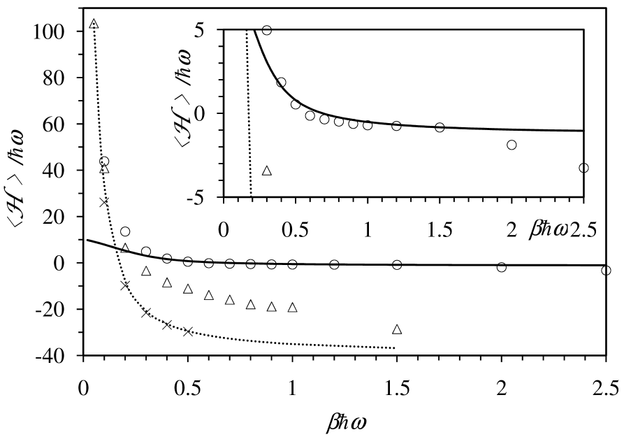
Figure 3 also includes the result of a high temperature expansion for the commutation function. Attard19b Although the terms in this expansion are formally exact, it can be seen that the result is practically indistinguishable from the classical result on the scale of the figure. Given the complexity of the terms and the brute force nature of the expansion, this does not appear to be a promising approach for the quantitative description of quantum effects in terrestrial condensed matter.

Figure 4 shows the average energy for $N=5$ distinguishable particles. Again it can be seen (inset) that the slope and curvature of the energy curve given by the present theory agree with that derived from the eigenvalue data of Ref. [Hernando13, ] in the intermediate temperature regime, $0.4\lesssim\beta\hbar\omega\lesssim 1.5$. The present two neighbor local field approach, the harmonic local field approach (ie. mean field), and the high temperature expansion, all go over to the classical limit at high temperatures. The quadratic approximation to the local field again appears inadequate at lower temperatures. The ground state formula given above gives $E_{0}^{\mathrm{loc}}/\hbar\omega=-18.6$ for $N=5$, and the classical result at absolute zero is $\langle{\cal H}\rangle_{\mathrm{cl}}/\hbar\omega=-38.6$. The present result again appears to underestimate the shifted benchmark result, $E_{0}/\hbar\omega=-1.13$.

Its worth mentioning the earlier mean field (ie. harmonic local field) results for a quantum harmonic crystal for which the exact analytic results are known.Attard19a At the relatively low temperature of $\beta\hbar\omega_{\mathrm{LJ}}=10$, the singlet harmonic mean field approach gave $\langle{\cal H}\rangle/\hbar\omega_{\mathrm{LJ}}=3.116\pm.002$ and the pair mean field gave $3.305\pm.001$, to be compared to the exact classical result of 0.4, and the exact ground state energy of 3.385.Attard19b These show that the local field approach is quite capable of giving accurate results even at low temperatures where the quantum ground state is dominant. This is perhaps surprising since the local field Hamiltonian operator used in the harmonic calculations (and also here) is strictly valid only up to the linear term in a high temperature expansion. Apparently the approximate non-linear terms induced by the re-exponentiation produce accurate results also at low temperatures.

Density profiles at $\beta\hbar\omega=0.4$ are shown in Fig. 5. All three approaches give a density symmetrically localized about the mid-plane, as one would expect for the simple harmonic oscillator applied potential. All approaches also predict molecular-sized oscillations in the density profile, which is indicative of a relatively close-packed system. The outer peaks are less well-defined in the benchmark results than in the classical or present singlet local field approaches.

The high frequency oscillatory fine structure evident in the profile given by the present theory is statistically significant. It is not an artefact of the grids used to collect the density profile or to store the singlet commutation function. On the scale of the figure no difference would be seen for distinguishable particles, bosons, or fermions.

Figure 6 shows the density profiles at a lower temperature, $\beta\hbar\omega=0.7$. In this case the structure is much more well-defined, and the departure from classical close-packing is relatively small. It is remarkable just how much of the density structure is due to purely classical considerations even at this low temperature. Again the high frequency fine structure in the present density profile is statistically significant and it appears robust with respect to changes in the various grids and particle statistics used in the simulations.

References

- (1) P. Attard, Entropy Beyond the Second Law. Thermodynamics and Statistical Mechanics for Equilibrium, Non-Equilibrium, Classical, and Quantum Systems, (IOP Publishing, Bristol, 2018).
- (2) P. Attard, “Quantum Statistical Mechanics in Classical Phase Space. Expressions for the Multi-Particle Density, the Average Energy, and the Virial Pressure”, arXiv:1811.00730 [quant-ph] (2018).
- (3) E. Wigner, “On the Quantum Correction for Thermodynamic Equilibrium”, Phys. Rev. 40, 749 (1932).
- (4) J. G. Kirkwood, “Quantum Statistics of Almost Classical Particles”, Phys. Rev. 44, 31 (1933).
- (5) P. Attard, “Quantum Statistical Mechanics as an Exact Classical Expansion with Results for Lennard-Jones Helium”, arXiv:1609.08178v3 [quant-ph] (2016).
- (6) P. Attard, “Quantum Statistical Mechanics in Classical Phase Space. Test Results for Quantum Harmonic Oscillators”, arXiv:1811.02032 (2018).
- (7) P. Attard, “Quantum Monte Carlo in Classical Phase Space. Mean Field and Exact Results for a One Dimensional Harmonic Crystal”, arXiv:1904.10650 (2019).
- (8) P. Attard, “Quantum Statistical Mechanics in Classical Phase Space. III. Mean Field Approximation Benchmarked for Interacting Lennard-Jones Particles”, arXiv:1812.03635 [quant-ph] (2018).
- (9) P. Attard, “Quantum Ornstein-Zernike Equation”, arXiv:1908.06373v2 [quant-ph] (2019).
- (10) A. Hernando and J. Vaníček, “Imaginary-time nonuniform mesh method for solving the multidimensional Schrödinger equation: Fermionization and melting of quantum Lennard-Jones crystals”, Phys. Rev. A 88, 062107 (2013). arXiv:1304.8015v2 [quant-ph] (2013).
- (11) A. Messiah, Quantum Mechanics, (North-Holland, Amsterdam, Vols I and II, 1961).
- (12) P. Attard, “Fermionic Phonons: Exact Analytic Results and Quantum Statistical Mechanics for a One Dimensional Harmonic Crystal”, arXiv:1903.06866 [quant-ph] (2019).
Appendix A Higher Order Corrections
In § II.2.1 it was shown that the effective local field gave a singlet Hamiltonian operator that coincided with the actual Hamiltonian operator exactly to linear order. This appendix derives the correction to this singlet operator that makes it exact to quadratic order in the expression for the commutation function. Here and throughout the gradient operator means a derivative with respect to , and these are all performed before setting equal to .
The exact and effective potentials differ in the gradient of the pair potential. For the pair part of the exact Hamiltonian one has