Quantum phases of dipolar bosons in one-dimensional optical lattices
Abstract
We theoretically analyze the phase diagram of a quantum gas of bosons that interact via repulsive dipolar interactions. The bosons are tightly confined by an optical lattice in a quasi one-dimensional geometry. In the single-band approximation, their dynamics is described by an extended Bose-Hubbard model where the relevant contributions of the dipolar interactions consist of density-density repulsion and correlated tunneling terms. We evaluate the phase diagram for unit density using numerical techniques based on the density-matrix renormalization group algorithm. Our results predict that correlated tunneling can significantly modify the parameter range of the topological insulator phase. At vanishing values of the onsite interactions, moreover, correlated tunneling promotes the onset of a phase with a large number of low energy metastable configurations.
I Introduction
Quantum gases of atoms and molecules in optical lattices are formidable platforms for studying the emergence of complex states of matter from the dynamics of the individual constituents, thanks to the experimental control of the characteristic length and energy scales Bloch et al. (2008); Gross and Bloch (2017). One prominent example is the observation of the quantum phase transition between Mott-insulator and superfluid phases Fisher et al. (1989); Greiner et al. (2002), demonstrating that these systems are versatile quantum simulators of the Bose-Hubbard model Bloch et al. (2008). The most recent confinement of ultracold dipolar gases in optical lattices Baier et al. (2016) and the combination of optical lattices and cavity setups Landig et al. (2016) has permitted to study the interplay between short and long-range interactions in these settings. These experiments reported dynamics that can be encompassed by the so-called extended Bose-Hubbard models Dutta et al. (2015), where these interactions are described by additional terms of the Bose-Hubbard Hamiltonian Sowiński et al. (2012); Habibian et al. (2013); Caballero-Benitez and Mekhov (2015).
In a lattice the effect of a two-body potential results in interaction terms, proportional to the onsite densities on both contributing lattice sites, as well as in so-called correlated tunneling terms, where hopping from site to site depends on the occupation of the neighboring sites Sowiński et al. (2012); Dutta et al. (2015); Cartarius et al. (2017). Detailed studies of the extended Bose-Hubbard model for dipolar gases typically included only the density-density interaction terms. These terms can induce density modulations and, in one dimension and at unit density, are responsible for the emergence of the so-called Haldane topological insulator, namely, an incompressible phase with a non-local order parameter Batrouni et al. (2013, 2014); Rossini and Fazio (2012); Dalla Torre et al. (2006); Kawaki et al. (2017).
Correlated tunneling is known from studies of superconductivity Strack and Vollhardt (1993); Hirsch (1994); Amadon and Hirsch (1996) and quantum magnets Schmidt et al. (2006). In quantum gases of bosons, at sufficient large dipolar interaction strengths it gives rise to pair condensation Schmidt et al. (2006); Sowiński et al. (2012) and to superfluidity with complex order parameter Jürgensen et al. (2015). Recent works showed that correlated tunneling is responsible for the emergence of superfluidity at large onsite repulsions, where one would instead expect insulating phases Biedroń et al. (2018); Kraus et al. (2020); Suthar et al. (2020). The effect of correlated tunneling for large densities in an one-dimensional lattice was studied in Ref. Kraus et al. (2020); Biedroń et al. (2018) and its two-dimensional extension was examined in Ref. Suthar et al. (2020). In particular, preliminary studies of the influence of the correlated tunneling on the existence of the Haldane insulator for a certain parameter choice was performed in Biedroń et al. (2018).
In this work we perform an extensive characterization of the effect of correlated tunneling on the ground state of dipolar gases in (quasi) one dimension for unit density, focusing in particular on the existence and properties of the Haldane insulator. For this purpose we numerically determine the phase diagram of the extended Bose-Hubbard model in one dimension and at unit density. We focus on the parameter regime where the Haldane insulating phase was predicted in Refs. Batrouni et al. (2013, 2014); Rossini and Fazio (2012); Dalla Torre et al. (2006); Kawaki et al. (2017) and, differing from those works, we systematically include correlated tunneling into our model. Motivated by recent experiments with low dimensional dipolar gases in optical lattices Baier et al. (2016); de Paz et al. (2013); Moses et al. (2015); Covey et al. (2016); Reichsöllner et al. (2017); Moses et al. (2016); Bohn et al. (2017), we take care of linking the coefficients of the extended Bose-Hubbard model with the experimental control parameters, in order to preserve the correct scaling between the coefficients across the phase diagram. The phase diagram is evaluated by means of the Density Matrix Renormalization Group (DMRG) approach White (1992, 1993); Orús (2014); Schollwöck (2011) and of its version simulating the thermodynamic limit, here referred to as the infinite DMRG (iDMRG) Schollwöck (2011); McCulloch ; Crosswhite et al. (2008); Kjäll et al. (2013).
This paper is organized as follows. In Sec. II we introduce the model, the extended Bose-Hubbard model for bosons interacting via onsite repulsion, nearest-neighbor repulsive interactions and nearest-neighbor correlated tunnelings. We then discuss the connection between the coefficients of the extended Bose-Hubbard model and the experimental realizations in quasi one-dimensional geometries. In Sec. III we analyze the resulting ground-state phase diagram for unit density. The conclusions are drawn in Sec. IV. The appendices provide details on the numerical implementations.
II Extended Bose-Hubbard model
The model at the basis of our analysis is the one-dimensional extended Bose-Hubbard Hamiltonian , that reads Sowiński et al. (2012); Cartarius et al. (2017):
where the first line is the standard Bose-Hubbard model and the second line is due to additional nearest-neighbor interactions. Here, is the number of sites, the operators and annihilate and create, respectively, a boson at site , with , and the operator counts the bosons at site . The coefficients are assumed to be real. Specifically, the tunneling rate describes the nearest-neighbor hopping, which promotes superfluidity, and . The onsite repulsion , , penalizes multiple occupation of a single site. In the "standard" Bose-Hubbard model, as given by the first line of Eq. (II), the ratio controls the phase transition from superfluidity (SF) to Mott-Insulator (MI) at commensurate densities Fisher et al. (1989).
The second line of Eq. (II) contains the terms due to the dipolar interactions. The term proportional to describes density-density interactions that favor the formation of density modulations in the repulsive, , case Menotti et al. (2007). The last term is responsible for tunneling processes that depend on the density of the neighboring sites and are scaled by the coefficient . Here, we have omitted a pair tunneling term and 4-site scattering terms, since the corresponding coefficients are of higher order in the Bose-Hubbard expansion Dutta et al. (2011); Biedroń et al. (2018); Kraus et al. (2020). Moreover, we have omitted terms beyond nearest neighbors. These additional terms can significantly modify the phase diagram for large values of Kraus et al. (2020), but give rise to small corrections for the parameters considered in this work.
II.1 Order parameters
We characterize the ground-state phase diagram of Hamiltonian (II) by means of the observables that we detail in what follows. We first determine the ground state energy for particle over lattice sites, with . The so-called charge gap corresponds to the energy required to create a particle-hole pair and is obtained after finding the ground-state energies for and bosons Batrouni et al. (2013, 2014):
| (2) |
Its non-vanishing value in the thermodynamic limit signals an insulating phase. An insulator is also characterized by a finite value of the so-called neutral gap , corresponding to the difference between the energy of the first excited state and the energy of the ground state Batrouni et al. (2013, 2014):
| (3) |
The first excited state is numerically found by determining the lowest energy state in the subspace orthogonal to the ground state, see Appendix A. In the SF phase the neutral gap vanishes in the thermodynamic limit.
We note that in one dimension the SF phase is strictly-speaking a Luttinger liquid with exponent Biedroń et al. (2018); Deng et al. (2013); Batrouni et al. (2014); Cazalilla et al. (2011), thus the off-diagonal correlations decay with the distance according to a power-law:
| (4) |
In order to reveal modulations in the off-diagonal correlations, we calculate the Fourier transform of the single-particle density matrix :
| (5) |
Typically, in a standard SF the maximum component of is at . The correlated tunneling, on the other hand, gives rise to effects that in one dimension are analogous to an effective change of the sign of the tunneling coefficient. Correspondingly, the Fourier transform of the single-particle density matrix can have a non-zero component at . We dub the corresponding ground state as staggered superfluid (SSF) phase Kraus et al. (2020).
| Phase | Acronym | Charge gap | Neutral gap | Fourier trans. | Density modulation | String order | String order | Parity order |
|---|---|---|---|---|---|---|---|---|
| , Eq. (2) | , Eq. (3) | , Eq. (5) | , Eq. (6) | , Eq. (7) | , Eq. (7) | , Eq. (8) | ||
| Mott Insulator | MI | |||||||
| Charge Density Wave | CDW | |||||||
| Haldane Insulator | HI | |||||||
| Lattice Superfluid | SF | |||||||
| Lattice Supersolid | SS | |||||||
| Lattice staggered Superfluid | SSF | |||||||
| Lattice staggered Supersolid | SSS |
Density modulated phases are revealed by properties of the local density-density correlations Rossini and Fazio (2012); Berg et al. (2008), whose Fourier transform is the structure form factor:
| (6) |
For a two-site translational symmetry, shows a finite peak at . The phase is a Charge Density Wave (CDW) or lattice Supersolid (SS) depending on whether the density-modulated phase is incompressible or superfluid, respectively. The SS phase is a staggered supersolid (SSS) when is finite and maximum at .
The Haldane insulating phase (HI) is gapped and characterized by non-local spatial correlations in the density fluctuations . This is captured by the string order parameter Batrouni et al. (2014); Dalla Torre et al. (2006); Berg et al. (2008); Batrouni et al. (2013); Rossini and Fazio (2012):
| (7) | |||
The definition of the density fluctuation is important. When we consider the density fluctuations about the mean value , namely, , then we label the string order parameter by . When instead the density fluctuations are taken about the local mean occupation , namely, , then the corresponding string order parameter is given by . Both definitions give finite values within the HI phase. Instead, in the CDW phase vanishes, while is finite. Thus signals the HI phase. The HI phase can also be distinguished from other insulating phases by means of the parity order parameter
| (8) | |||
which is finite in the MI and CDW phases, while it vanishes in the HI phase independent of the definition of .
The phases and the corresponding values of order parameters are summarized in Table 1.
Finally, we determine the von-Neumann entropy of the ground state for a lattice bipartition into two subsystems and . Denoting the ground state by , the von-Neumann (entanglement) entropy is defined as Amico et al. (2008); Eisert et al. (2010); Metlitski and Grover ; Frérot and Roscilde (2016)
| (9) |
where .
II.2 Bose-Hubbard coefficients
The extended Bose-Hubbard model of Eq. (II) is a good approximation of the Hamiltonian describing the dynamics of dipolar atoms tightly confined by the lowest band of an optical lattice in a quasi one-dimensional geometry. The trapping potentials can be described by a potential of the form:
| (10) |
where is the atomic mass, is the frequency of the harmonic trap that confines the atomic motion along the direction, and is the depth of the optical lattice with periodicity . The details of the derivation of Eq. (II), starting from the full Hamiltonian of interacting atoms in the potential of Eq. (10), have been extensively reported, for instance, in Refs. Cartarius et al. (2017); Kraus et al. (2020). These derivations allow one to link the Bose-Hubbard coefficients with the experimental parameters.
In this work we set and with and the recoil energy for a laser with wavelength . The choice of warrants that the transverse motion is frozen out for the parameters that we consider. Since we keep the depth constant, the tunneling amplitude is fixed and finite.
We sweep across the insulator-superfluid transition by varying the onsite interaction coefficient . The latter results from the interplay between the van-der-Waals, contact potential and the onsite contribution of the dipolar interaction :
| (11) | |||
| (12) |
Here, and is tuned by changing the scattering length, while the dipole-dipole potential is scaled by the coefficient and denotes the angle between the dipoles and the interparticle distance vector . The other coefficients and are changed by varying the dipolar strength.
Figure 1 displays the absolute value of the correlated tunneling coefficient, , as a function of the nearest-neighbor interaction, , and of the onsite interaction, . Both coefficients as well as increase with the dipole-dipole interaction strength, which is here reported in terms of the dimensionless parameter Biedroń et al. (2018); Astrakharchik et al. (2007):
| (13) |

Note that is negative for the parameters we consider and it scales as .
III Ground-state phase diagram
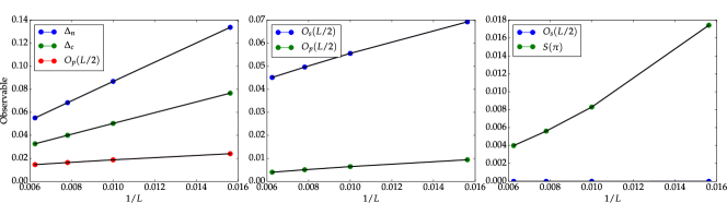
In this section we analyze the properties of the ground state of the extended Bose-Hubbard Hamiltonian in the -plane and for the unit density. We numerically determine the ground state on a finite lattice by means of DMRG and extrapolate to the thermodynamic limit of a given observable according to the procedure Batrouni et al. (2014); Rossini and Fazio (2012):
| (14) |
where and are constants, and stands for the observable at the lattice length (see Appendix A). In our numerical simulations we take . We identify the phase boundaries following the prescription given in Table 1 for different observables. In this procedure we neglect the outer sites at both edges of the lattice in order to get rid of boundary effects and we evaluate the order parameters in the central part of the lattice, which consists of sites Batrouni et al. (2014); Rossini and Fazio (2012) (see Appendix A). We compare these results with the phase diagram determined using iDMRG i.e., in the direct thermodynamic limit. Details of the implementations are provided in Appendix A.
III.1 Phase diagram

The phase diagram for the density is shown in Fig. 2 for a finite chain. The different colors indicate the phase boundaries predicted by (i) the charge gap (blue), (ii) the neutral gap (magenta), (iii) the string order parameter (red), (iv) the parity order parameter (black) and (v) the CDW order parameter (green). The boundaries are extracted following the procedure described above, using Eq. (14).
In the considered parameter regime the phases are SF, MI, HI, CDW, and a region which has the features of a phase separation (PS) and which will be discussed in Sec. III.4. We note that we do not find any staggered SF. These findings are in agreement with the results obtained with infinite DMRG. Figure 3 displays a color plot of the string order parameter , (7) and of the parity order parameter , (8), both obtained with iDMRG. For comparison, we also report the corresponding values obtained by setting .
Despite some similarities with the phase diagram found setting in Eq. (II) Batrouni et al. (2013, 2014); Rossini and Fazio (2012), nevertheless, there are also some striking differences. In the first place, for the HI phase occupies a smaller area in parameter space. This confirms the observation in Ref. Biedroń et al. (2018). In general, correlated tunneling stabilizes the MI and CDW phases in the parameter space, while the size of SF and HI phases are substantially reduced. Moreover, the HI phase seems to stretch down to smaller values of and . We note that we cannot determine the phase boundaries for small and around because in this region the error bars are large.

III.2 The von-Neumann entropy
The color plots in Fig. 4 report the von-Neumann entropy, (9), across the phase diagram and calculated by means of iDMRG. The von-Neumann entropy sheds light on the spatial decay of correlations. Comparison with the plot of the Fourier transform of the single-particle density matrix, Fig. 5, shows that part of the region where is maximal overlaps with the SF domain. Like , the von-Neumann entropy decays slowly to zero when increasing at small values of , sweeping across the SF-MI phase transition.


For small and for undergoes strong fluctuations from point to point. We associate this behavior with the phase separation where the convergence of DMRG is doubtful. Comparing this region with the one at , lower panel of Fig. 4, we observe that for it appears at significantly lower values of .

Figure 6 displays as a function of at fixed ratio , in the part of the phase diagram where the phases are insulating. Starting from the MI phase we observe peaks when crossing the MI-HI and the HI-CDW transitions, which we discuss in detail in the following.


III.3 MI-HI-CDW transitions
In Fig. 2 we observe a direct transition from the MI to the CDW phase at sufficiently high values of . Fig. 7 shows that string () and density-wave order () parameters are discontinuous at the transition point, indicating a first-order phase transition. Here the string and density-wave order parameter agree almost exactly, since in the limit large the MI and CDW can be described by trivial Fock states, which lead to the same value of the string and density-wave order parameter in the thermodynamic limit.
At smaller values of the ratio the HI phase separates the MI from the CDW phase. The peaks in the profile of the von-Neumann entropy in Fig. 6 suggest that the phase transitions at the MI-HI and at the HI-CDW transitions are continuous (of second order). This is corroborated by the behavior of the neutral gap at the MI-HI and at the HI-CDW transitions. The HI phase corresponds to the interval where the energy gaps and the string order parameter possess finite values, while both parity and density-wave order parameter vanish. The finite value of the string order parameter and the vanishing parity order parameter demonstrate the topological nature of the HI phase.
The neutral and charge gaps are displayed in the lower panel of Fig. 8 for as a function of . For small the neutral and charge gaps are finite, corresponding to the MI phase. For a larger value of the gaps shrink to zero indicating the continuous transition to the HI phase. This agrees with the results for the case (no correlated tunneling) Batrouni et al. (2014); Berg et al. (2008); Ejima and Fehske (2015); Ejima et al. (2014), where vanishing gaps both in the charge and neutral sectors signal a second order phase transition with central charge Berg et al. (2008); Ejima et al. (2014); Ejima and Fehske (2015). At the transition separating the HI and the CDW (symmetry-broken) phase the neutral gap vanishes, while the charge gap remains finite. This is as in the case, where the transition is of Ising type with central charge Berg et al. (2008); Amico et al. (2010); Ejima et al. (2014); Ejima and Fehske (2015) and the quantum critical point is topological Fraxanet et al. (2022). In the CDW phase the density-wave order parameter reaches a finite value, see the upper panel of Fig. 8.


III.4 Phase separation
We finally discuss the parameter region at large but small , where the von-Neumann entropy has large fluctuations from point to point. We denote this regime by phase separation. Here, we find that the ground state of the canonical ensemble consists of a mixture of two or more phases. This feature can be revealed by inspecting the site occupation and its variance across the lattice. It can also be captured by the chemical potential as a function of the density Batrouni et al. (2014); Maik et al. (2013). In fact, in the grand-canonical ensemble the phase at unit density is unstable and the density is a discontinuous function of the chemical potential Batrouni et al. (2014).
In order to analyze the phase-separation region in the canonical ensemble, we calculate the density as a function of the chemical potential , which we find by means of the formula Batrouni et al. (2014)
| (15) |
Figure 9 displays as a function of for within the phase-separation region. The behavior suggests a hysteresis, which signals a discontinuous transition.

The phase separation region for has been recently extensively analyzed in Kottmann et al. (2021). Correlated tunneling shifts the appearance of this phase to lower values of and possibly increases the number of metastable configurations. Figure 10 displays some of the metastable configurations we find, corresponding to CDW clusters separated by SF regions. Configurations like the one in the upper panel have been reported in Batrouni et al. (2014). The configuration in the lower panel, instead, seems to be stable due the presence of correlated tunneling.

III.5 Discussion
In previous works some of us showed that the effect of correlated tunneling on the ground-state phase diagram can be partially captured by an effective model. In this effective model correlated tunneling and single-particle hopping are replaced in Eq. (II) by a single hopping term with effective tunneling coefficient Kraus et al. (2020); Suthar et al. (2020). This coefficient can vanish, giving rise to an effective atomic limit which agrees with numerical results obtained with the full model Kraus et al. (2020); Suthar et al. (2020). We have verified that, for the parameters we consider, is always finite. Fig. 11 displays the same data as in Fig. 2, but with the axes now rescaled by : The rescaled phase boundaries SF-MI and MI-HI-CDW are in good agreement with the phase diagram at (c.f. Fig. 6(b)) Batrouni et al. (2014), suggesting that the effect of correlated tunneling on the size of the insulating phase could be captured by this effective description.

IV Conclusion
We have analyzed the ground-state phase diagram of the extended Bose-Hubbard model in one dimension and unit density, describing a gas of dipolar bosons in an optical lattice and in a quasi one-dimensional geometry. With respect to previous studies, in this work we have performed a systematic characterization of the effect of correlated tunneling on the phase diagram, focusing in particular on the parameter regime of the topological Haldane insulator.
For the considered parameter space correlated tunneling plays a relevant role in determining the essential features of the phase diagram. By comparing with the phase diagrams calculated setting Batrouni et al. (2013, 2014); Rossini and Fazio (2012); Berg et al. (2008), we find that correlated tunneling tends to stabilize the insulating phases and to shrink the parameter region where the Haldane insulator is found. Moreover, correlated tunneling promotes the onset of the phase-separation regime also at relatively low values of the dipolar interactions, giving rise to a large number of low-energy metastable configurations. Future work will analyses relaxation after quenches. In fact, the Bose-Hubbard model with correlated tunneling exhibits several analogies with constrained models, which are known to give rise to a rich prethermalization dynamics Nuske et al. (2020); Bluvstein et al. (2021); Ney et al. (2022).
This study shows that correlated tunneling gives rise to correlations which are only partially captured by the observables typically employed for characterizing the phase diagram. These correlations might be also important at fractional filling. For instance, they might affect the properties of the Fibonacci anyonic excitations expected at for low tunneling rates Đurić et al. (2017).
Acknowledgements.
The authors are grateful to Benoit Gremaud, and Luis Santos for discussions and especially to George Batrouni for helpful comments. RK and GM acknowledge support by the Deutsche Forschungsgemeinschaft (DFG, German Research Foundation) via the CRC-TRR 306 “QuCoLiMa”, Project-ID No. 429529648, and by the priority program No. 1929 "GiRyd”’. We also thank funding by the German Ministry of Education and Research (BMBF) via the QuantERA project NAQUAS. Project NAQUAS has received funding from the QuantERA ERA-NET Cofund in Quantum Technologies implemented within the European Union’s Horizon 2020 program. TC and JZ thank the support of PL-Grid Infrastructure and the National Science Centre (Poland) under project Opus 2019/35/B/ST2/00034 (J.Z.) and Unisono 2017/25/Z/ST2/03029 (T.C.) realized within QuantERA ERA-NET QTFLAG collaboration.Appendix A Details on the DMRG algorithm
The phase diagrams are calculated by means of a DMRG numerical program using the ITensor C++ library Fishman et al. (see also Ref. Kraus et al. (2020))) and using infinite DMRG (iDMRG) method available in TeNPy library Hauschild and Pollmann (2018).
A.1 DMRG for finite chains
For the finite chain we lift the degeneracy in the CDW phase and Haldane phase by adding the boundary term . The maximal bond dimension is set to , the energy error goal is fixed to and the upper limit for the singular values discarded is set to . We allow for maximally particles per site. In order to ensure that the simulations end up in the ground state we run the simulation for three different initial states: the CDW state
| (16) |
with and , the MI state and a random initial state. The random state is a superposition of Fock states , where is chosen randomly out of the interval with the constrain . We choose the number of superimposed Fock state to be . We note that the string order parameter , Eq. (7), and the structure form factor, Eq. (6), at have the same value for the CDW Fock state (see Eq. (16)) modulo a term proportional to and which vanishes in the limit . In order to calculate the first excited state one adds an extra term to the Hamiltonian, which lifts the energy of the ground state:
| (17) |
with the ground state. The first excited state is determined by calculating the ground state of in Eq. (17) using the DMRG ground state algorithm. The weight of the extra term is chosen to be .
We determine the ground state by means of this DMRG numerical program and calculate the observables presented in Sec. II.1. In order to get rid of the boundary effect we neglect the outer sites in the determination of the observables following Rossini and Fazio (2012); Batrouni et al. (2014). To justify this cut we show in Fig. 12 the string order parameter, (7), as a function of the number of lattice sites cut at the boundary together with the value of the order parameter calculated by means of iDMRG. For a systematic analysis of the effect of the boundary conditions see Stumper and Okamoto (2020).


To get the phase diagram in the thermodynamic limit we fit the values of the observables for different numbers of lattice sites according to (14). We justify the application of Eq. (14) by inspecting the observables as a function of . Fig. 13 shows the neutral gap (3), the charge gap (2), and the parity order parameter (8) as a function of near the SF-MI phase transition at . The gaps follow a linear behavior as function of near the SF-MI transition. Moreover, Fig. 13 shows the behavior of the observables as a function of at the HI-MI and MI-CDW transition, where the observables dependence is nicely fitted by (14).
We identified the boundary lines in Figures 1, 3, 4 and 5 by using a certain threshold value for the order parameter above which we determine a certain phase. Those threshold values are those, who reproduce the critical value of the MI-SF transition at in Ref. Kühner et al. (2000) and the SF-HI transition at in Ref. Batrouni et al. (2014). Here we make use of our data set for . We then convert the error corresponding to the fitting procedure into an error in the phase boundary. Fig. 13 displays the phase boundaries in the -plane including the error bars for each point at the phase boundary.

A.2 iDMRG simulations
We also explore the system directly at the thermodynamic limit using the infinite DMRG (iDMRG) algorithm McCulloch ; Crosswhite et al. (2008); Kjäll et al. (2013) based on translationally invariant infinite matrix-product state (iMPS) ansatz Vidal (2007). Since the onset of the CDW phase requires unit cells of size integer multiple of 2, we consider iMPS representation with unit cells of size 4 for our simulations. The maximum bosonic occupancy is taken to be . We fix the maximal iMPS bond dimension to and checked that our results do not change by changing the bond dimension to . To confirm the convergence of the iDMRG algorithm, we follow the change in energy density in successive iDMRG sweeps, and when the change falls below , we conclude that the resulting iMPS is the ground state of the infinite system.
References
- Bloch et al. (2008) I. Bloch, J. Dalibard, and W. Zwerger, Rev. Mod. Phys. 80, 885 (2008).
- Gross and Bloch (2017) C. Gross and I. Bloch, Science 357, 995 (2017).
- Fisher et al. (1989) M. P. A. Fisher, P. B. Weichman, G. Grinstein, and D. S. Fisher, Phys. Rev. B 40, 546 (1989).
- Greiner et al. (2002) M. Greiner, O. Mandel, T. Esslinger, T. W. Hänsch, and I. Bloch, Nature 415, 39 (2002).
- Baier et al. (2016) S. Baier, M. J. Mark, D. Petter, K. Aikawa, L. Chomaz, Z. Cai, M. Baranov, P. Zoller, and F. Ferlaino, Science 352, 201 (2016).
- Landig et al. (2016) R. Landig, L. Hruby, N. Dogra, M. Landini, R. Mottl, T. Donner, and T. Esslinger, Nature 532, 476 (2016).
- Dutta et al. (2015) O. Dutta, M. Gajda, P. Hauke, M. Lewenstein, D.-S. Lühmann, B. A. Malomed, T. Sowiński, and J. Zakrzewski, Reports on Progress in Physics 78, 066001 (2015).
- Sowiński et al. (2012) T. Sowiński, O. Dutta, P. Hauke, L. Tagliacozzo, and M. Lewenstein, Phys. Rev. Lett. 108, 115301 (2012).
- Habibian et al. (2013) H. Habibian, A. Winter, S. Paganelli, H. Rieger, and G. Morigi, Phys. Rev. Lett. 110, 075304 (2013).
- Caballero-Benitez and Mekhov (2015) S. F. Caballero-Benitez and I. B. Mekhov, Phys. Rev. Lett. 115, 243604 (2015).
- Cartarius et al. (2017) F. Cartarius, A. Minguzzi, and G. Morigi, Phys. Rev. A 95, 063603 (2017).
- Batrouni et al. (2013) G. G. Batrouni, R. T. Scalettar, V. G. Rousseau, and B. Grémaud, Phys. Rev. Lett. 110, 265303 (2013).
- Batrouni et al. (2014) G. G. Batrouni, V. G. Rousseau, R. T. Scalettar, and B. Grémaud, Phys. Rev. B 90, 205123 (2014).
- Rossini and Fazio (2012) D. Rossini and R. Fazio, New Journal of Physics 14, 065012 (2012).
- Dalla Torre et al. (2006) E. G. Dalla Torre, E. Berg, and E. Altman, Phys. Rev. Lett. 97, 260401 (2006).
- Kawaki et al. (2017) K. Kawaki, Y. Kuno, and I. Ichinose, Phys. Rev. B 95, 195101 (2017).
- Strack and Vollhardt (1993) R. Strack and D. Vollhardt, Phys. Rev. Lett. 70, 2637 (1993).
- Hirsch (1994) J. Hirsch, Physica B: Condensed Matter 199-200, 366 (1994).
- Amadon and Hirsch (1996) J. C. Amadon and J. E. Hirsch, Phys. Rev. B 54, 6364 (1996).
- Schmidt et al. (2006) K. P. Schmidt, J. Dorier, A. Läuchli, and F. Mila, Phys. Rev. B 74, 174508 (2006).
- Jürgensen et al. (2015) O. Jürgensen, K. Sengstock, and D.-S. Lühmann, Scientific Reports 5, 12912 (2015).
- Biedroń et al. (2018) K. Biedroń, M. Łącki, and J. Zakrzewski, Phys. Rev. B 97, 245102 (2018).
- Kraus et al. (2020) R. Kraus, K. Biedroń, J. Zakrzewski, and G. Morigi, Phys. Rev. B 101, 174505 (2020).
- Suthar et al. (2020) K. Suthar, R. Kraus, H. Sable, D. Angom, G. Morigi, and J. Zakrzewski, Phys. Rev. B 102, 214503 (2020).
- de Paz et al. (2013) A. de Paz, A. Sharma, A. Chotia, E. Maréchal, J. H. Huckans, P. Pedri, L. Santos, O. Gorceix, L. Vernac, and B. Laburthe-Tolra, Phys. Rev. Lett. 111, 185305 (2013).
- Moses et al. (2015) S. A. Moses, J. P. Covey, M. T. Miecnikowski, B. Yan, B. Gadway, J. Ye, and D. S. Jin, Science 350, 659 (2015).
- Covey et al. (2016) J. P. Covey, S. A. Moses, M. Gärttner, A. Safavi-Naini, M. T. Miecnikowski, Z. Fu, J. Schachenmayer, P. S. Julienne, A. M. Rey, D. S. Jin, and J. Ye, Nature Communications 7, 11279 (2016).
- Reichsöllner et al. (2017) L. Reichsöllner, A. Schindewolf, T. Takekoshi, R. Grimm, and H.-C. Nägerl, Phys. Rev. Lett. 118, 073201 (2017).
- Moses et al. (2016) S. A. Moses, J. P. Covey, M. T. Miecnikowski, D. S. Jin, and J. Ye, Nature Physics 13, 13 (2016).
- Bohn et al. (2017) J. L. Bohn, A. M. Rey, and J. Ye, Science 357, 1002 (2017).
- White (1992) S. R. White, Phys. Rev. Lett. 69, 2863 (1992).
- White (1993) S. R. White, Phys. Rev. B 48, 10345 (1993).
- Orús (2014) R. Orús, Annals of Physics 349, 117 (2014).
- Schollwöck (2011) U. Schollwöck, Annals of Physics 326, 96 (2011).
- (35) I. P. McCulloch, “Infinite size density matrix renormalization group, revisited,” arXiv:0804.2509 .
- Crosswhite et al. (2008) G. M. Crosswhite, A. C. Doherty, and G. Vidal, Phys. Rev. B 78, 035116 (2008).
- Kjäll et al. (2013) J. A. Kjäll, M. P. Zaletel, R. S. K. Mong, J. H. Bardarson, and F. Pollmann, Phys. Rev. B 87, 235106 (2013).
- Menotti et al. (2007) C. Menotti, C. Trefzger, and M. Lewenstein, Phys. Rev. Lett. 98, 235301 (2007).
- Dutta et al. (2011) O. Dutta, A. Eckardt, P. Hauke, B. Malomed, and M. Lewenstein, New Journal of Physics 13, 023019 (2011).
- Deng et al. (2013) X. Deng, R. Citro, E. Orignac, A. Minguzzi, and L. Santos, Phys. Rev. B 87, 195101 (2013).
- Cazalilla et al. (2011) M. A. Cazalilla, R. Citro, T. Giamarchi, E. Orignac, and M. Rigol, Rev. Mod. Phys. 83, 1405 (2011).
- Berg et al. (2008) E. Berg, E. G. Dalla Torre, T. Giamarchi, and E. Altman, Phys. Rev. B 77, 245119 (2008).
- Amico et al. (2008) L. Amico, R. Fazio, A. Osterloh, and V. Vedral, Rev. Mod. Phys. 80, 517 (2008).
- Eisert et al. (2010) J. Eisert, M. Cramer, and M. B. Plenio, Rev. Mod. Phys. 82, 277 (2010).
- (45) M. A. Metlitski and T. Grover, “Entanglement entropy of systems with spontaneously broken continuous symmetry,” arXiv:1112.5166 .
- Frérot and Roscilde (2016) I. Frérot and T. Roscilde, Phys. Rev. Lett. 116, 190401 (2016).
- Astrakharchik et al. (2007) G. E. Astrakharchik, J. Boronat, I. L. Kurbakov, and Y. E. Lozovik, Phys. Rev. Lett. 98, 060405 (2007).
- Ejima and Fehske (2015) S. Ejima and H. Fehske, Journal of Physics: Conference Series 592, 012134 (2015).
- Ejima et al. (2014) S. Ejima, F. Lange, and H. Fehske, Phys. Rev. Lett. 113, 020401 (2014).
- Amico et al. (2010) L. Amico, G. Mazzarella, S. Pasini, and F. S. Cataliotti, New Journal of Physics 12, 013002 (2010).
- Fraxanet et al. (2022) J. Fraxanet, D. González-Cuadra, T. Pfau, M. Lewenstein, T. Langen, and L. Barbiero, Phys. Rev. Lett. 128, 043402 (2022).
- Maik et al. (2013) M. Maik, P. Hauke, O. Dutta, M. Lewenstein, and J. Zakrzewski, New Journal of Physics 15, 113041 (2013).
- Kottmann et al. (2021) K. Kottmann, A. Haller, A. Acín, G. E. Astrakharchik, and M. Lewenstein, Phys. Rev. B 104, 174514 (2021).
- Nuske et al. (2020) M. Nuske, J. Vargas, M. Hachmann, R. Eichberger, L. Mathey, and A. Hemmerich, Phys. Rev. Research 2, 043210 (2020).
- Bluvstein et al. (2021) D. Bluvstein, A. Omran, H. Levine, A. Keesling, G. Semeghini, S. Ebadi, T. T. Wang, A. A. Michailidis, N. Maskara, W. W. Ho, S. Choi, M. Serbyn, M. Greiner, V. Vuletić, and M. D. Lukin, Science 371, 1355 (2021).
- Ney et al. (2022) P.-M. Ney, S. Notarnicola, S. Montangero, and G. Morigi, Phys. Rev. A 105, 012416 (2022).
- Đurić et al. (2017) T. Đurić, K. Biedroń, and J. Zakrzewski, Phys. Rev. B 95, 085102 (2017).
- (58) M. Fishman, S. White, and E. Stoudenmire, “The ITensor software library for tensor network calculations,” arXiv:2007.14822 .
- Hauschild and Pollmann (2018) J. Hauschild and F. Pollmann, SciPost Phys. Lect. Notes , 5 (2018), code available from https://github.com/tenpy/tenpy, arXiv:1805.00055 .
- Stumper and Okamoto (2020) S. Stumper and J. Okamoto, Phys. Rev. A 101, 063626 (2020).
- Kühner et al. (2000) T. D. Kühner, S. R. White, and H. Monien, Phys. Rev. B 61, 12474 (2000).
- Vidal (2007) G. Vidal, Phys. Rev. Lett. 98, 070201 (2007).