Quantum phase measurement of two-qubit states in an open waveguide

Ya. S. Greenberg [email protected] Novosibirsk State Technical University, Novosibirsk, Russia A. A. Shtygashev Novosibirsk State Technical University, Novosibirsk, Russia

Abstract

We present a new method for quantum state tomography within a single-excitation subspace of two-qubit states in an open waveguide. The system under investigation consists of three qubits in an open waveguide, separated by a distance comparable to the wavelength of the electromagnetic field. We show that the modulation of the frequency of the central ancillary qubit allows us to obtain unambiguous information about the initial phase difference $\varphi_{1}-\varphi_{3}$ of the edge qubits via the measurement of the evolution of their probability amplitudes.

Keywords: open quantum systems, two-qubit states, quantum state tomography, waveguides

I Introduction

Extracting information about the quantum state is an essential task in the benchmarks of quantum devices or quantum information algorithms. This is referred to as quantum state tomography (QST). As in the classical tomography, when we reconstruct a three dimensional image of the object by the use of its various projections on a two-dimensional plane, quantum state tomography reconstructs the state by the use of sequences of quantum gates and projective measurements Toninelli2019 . A consequence of projective measurements is that the state is destroyed, therefore these sequences should be implemented onto a set of identical quantum systems or onto the same system prepared repeatedly in the same state Schmied2016 . In circuit Quantum Electrodynamics (cQED) one can perform directly measurements in the energy basis of qubits, or equivalently, measurement of the z-projection on the Bloch sphere. These measurements are typically dispersive-shift based, where the resonance frequency of the readout resonator is qubit-state dependent Blais2004 . To obtain the two remaining projections, one implements $X$ and $Y$ gates prior to the measurement Steffen2006 . To reconstruct the state of a single qubit at least three different gates are needed, and the density matrix has three independent elements that can be reconstructed using the measurement results. For two qubits the problem is already considerably more resource-demanding, as the number of gates increases to 9 for a two qubit state, and the full density matrix has 15 independent elements that have to be determined Wallraff2006 .

Open quantum systems without additional resonators are of the special interest both experimentally Brehm2021 ; Forn-Diaz2017 ; Koshino2013 ; Mirhosseini2019 and theoretically Kornovan2015 ; Fang2014 ; Fang2015 ; Issah2021 ; Kockum2018 ; Albrecht2019 ; Greenberg2017 ; Sultanov2018 . In these systems interference effects appear when the distance between qubits is comparable to a characteristic wavelength. The interference is caused by the effective interaction between the qubits via virtual photons. There are several theoretical works devoted to mentioned interference effects Greenberg2015 ; vanLoo2013 , synchronization and superradiance Cattaneo2021 , as well as experimental realizations of long-distance interacting superconducting qubits Wen2019 ; Zhong2019 .

Here we investigate an open quantum system consisting of an open waveguide, two main qubits and one ancillary central qubit, and we restrict the Hilbert space to a single-excitation subspace. By employing frequency modulation of the ancillary qubit Silveri2017 we obtain a one-to-one mapping between the phase of the two qubit off-diagonal density matrix element in the single-excitation subspace and the measurement result in the energy basis. Thus, the quantum state could be reconstructed by two measurements: the $\sigma_{z}$ -components of the two qubits without modulation, to get the absolute values of the amplitude probabilities; and the $\sigma_{z}$ -components of two qubits with modulation, to get the phases of the amplitude probabilities.

In contrast to a common practice where for tomography reconstruction the gate pulses are applied to the measured qubits, in our method the measurement pulse is applied to the ancillary qubit. Until the projective measurements two qubits do not undergo any external influence.

The paper is structured as follows.

In Section II we obtain the time-dependent differential equations for the probability amplitudes $\beta_{1,2,3}(t)$ of the three qubits, which account for the modulation of the frequency of the central qubit.

The main results of the paper are described in Section III. In Subsection III.1 we consider the free evolution of three-qubit system. We show that the free evolution probabilities $|\beta_{1}(t)|^{2}$ and $|\beta_{3}(t)|^{2}$ depend on the phase difference $\varphi_{1}-\varphi_{3}$ . However, the population difference $|\beta_{1}(t)|^{2}-|\beta_{3}(t)|^{2}$ is phase independent. It is shown that from free evolution measurements we can find both the initial values of probability amplitudes $\beta_{1,3}(0)$ and the quantity $\cos{(\varphi_{1}-\varphi_{3})}$ . In Subsection III.2 we consider the solution of the equations obtained in Section II under frequency modulation, $f(t)\neq 0$ with the initial conditions $\left.{\beta_{1}(t)}\right|_{t=0}=\beta_{1}(0);\;\left.{\beta_{2}(t)}\right|_{t=0}=0;\;\left.{\beta_{3}(t)}\right|_{t=0}=\beta_{3}(0)$ . From the results obtained in this section, we may conclude that modulating the frequency of the second qubit allows us to obtain unambiguous information about the initial phase difference $\varphi_{1}-\varphi_{3}$ via the measurement of the evolution of the probability amplitudes $|\beta_{1}(t)|^{2}$ , $|\beta_{3}(t)|^{2}$ .

II Formulation of the problem

We consider a linear chain of three equally spaced qubits which are coupled to the photon field in an open waveguide (see Fig. 1).

Refer to caption — Figure 1: Schematic illustration of the single-excitation subspace for a three-qubit chain in an open waveguide. (a) One qubit is excited, while the other two qubits are in the ground state. (b) All three qubits are in the ground state and a single photon propagates in the waveguide.

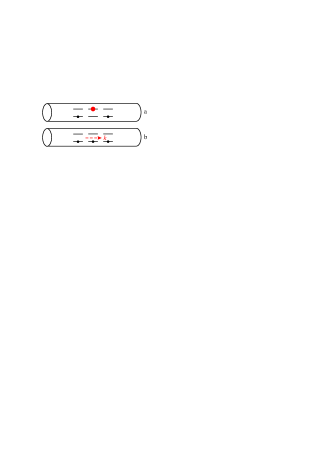
The distance between neighboring qubits is equal to $d$ . The Hilbert space of each qubit is spanned by the excited state vector $|e\rangle$ and the ground state vector $|g\rangle$ . The Hamiltonian that accounts for the interaction between qubits and the electromagnetic field is as follows (we use $\hbar=1$ throughout the paper):

H=H_{0}+\sum\limits_{k}{\omega_{k}a_{k}^{+}a_{k}}+H_{int}

(1)

where $H_{0}$ is the Hamiltonian of the bare qubits and $H_{\operatorname{int}}$ is the interaction Hamiltonian between the qubits and the photons in the waveguide

{H_{0}}=\frac{1}{2}\Omega\sum\limits_{n=1}^{3}{\left({1+\sigma_{z}^{\left(n\right)}}\right)}+\frac{1}{2}f\left(t\right)\left({1+\sigma_{z}^{\left(2\right)}}\right),

(2)

H_{\operatorname{int}}=\sum\limits_{n=1}^{3}{}\sum\limits_{k}{}g_{k}^{(n)}e^{-ikx_{n}}\sigma_{-}^{(n)}a_{k}^{+}+h.c..

(3)

In Eq. (2) the two edge qubits have equal frequencies, $\Omega$ , while the frequency of a central qubit, $\Omega_{C}(t)$ may be time-dependent: $\Omega_{C}(t)=f(t)+\Omega$ , i.e. detuned by $f(t)$ from the edge qubits. The quantity $g_{k}^{(n)}$ in Eq. (3) denotes the coupling between $n$ -th qubit and the photon field, while $x_{n}$ is the position of $n$ -th qubit.

Below we consider a single-excitation subspace with either a single photon in the waveguide and all qubits in the ground state, or with no photons in a waveguide and only one qubit in the chain being excited. The Hamiltonian Eq. (3) conserves the number of excitations (number of excited qubits + number of photons). Therefore, at any instant of time the system will remain within the single-excitation subspace. The wave function of an arbitrary single-excitation state can then be written in the form:

\left|\Psi(t)\right\rangle=\sum\limits_{n=1}^{3}{\beta_{n}(t)e^{-i\Omega t}}\left|{n,0_{k}}\right\rangle+\sum\limits_{k}{\gamma_{k}(t)e^{-i\omega_{k}t}}\left|{G,1_{k}}\right\rangle,

(4)

where $\beta_{n}(t)$ is the amplitude of $n$ -th qubit, $\left|{G,1_{k}}\right\rangle=\left|{g_{1},g_{2},g_{3}}\right\rangle\otimes\left|{1_{k}}\right\rangle$ , $\left|{1,0_{k}}\right\rangle=\left|{e_{1},g_{2},g_{3}}\right\rangle\otimes\left|{0_{k}}\right\rangle$ , $\left|{2,0_{k}}\right\rangle=\left|{g_{1},e_{2},g_{3}}\right\rangle\otimes\left|{0_{k}}\right\rangle$ , $\left|{3,0_{k}}\right\rangle=\left|{g_{1},g_{2},e_{3}}\right\rangle\otimes\left|{0_{k}}\right\rangle$ , and $\gamma_{k}(t)$ is a single-photon probability amplitude which is related to a spectral density of spontaneous emission.

The equations for the amplitudes $\beta_{n}(t)$ and $\gamma_{k}(t)$ in Eq. (4) can be found from the time-dependent Schrödinger equation $id|\Psi\rangle/dt=H|\Psi\rangle$ . For the probability amplitudes $\beta_{n}(t)$ we obtain the following equations (the details of the derivation are given in Appendix A):

\begin{gathered}\frac{{d\beta_{1}}}{{dt}}=-\frac{\Gamma}{2}\left({\beta_{1}+\beta_{2}e^{ikd}+\beta_{3}e^{i2kd}}\right)\hfill\\ \frac{{d\beta_{2}}}{{dt}}=-if(t)\beta_{2}(t)-\frac{\Gamma}{2}\left({\beta_{1}e^{ikd}+\beta_{2}+\beta_{3}e^{ikd}}\right)\hfill\\ \frac{{d\beta_{3}}}{{dt}}=-\frac{\Gamma}{2}\left({\beta_{1}e^{i2kd}+\beta_{2}e^{ikd}+\beta_{3}}\right),\hfill\\ \end{gathered}

(5)

where $k=\Omega/v_{g}$ and $\Gamma$ is the rate of spontaneous emission of qubit into the waveguide mode.

The wave function which describing the dynamic evolution of the $\beta_{n}(t)$ ’s is the projection of the single- excitation wavefunction Eq. (4) on the vacuum photon state:

\left|\Psi(t)\right\rangle_{0}=\left\langle{0_{k}|\Psi(t)}\right\rangle=\sum\limits_{n=1}^{3}{\beta_{n}(t)}\left|n\right\rangle.

(6)

where $\left|{\left.n\right\rangle}\right.=\left\langle{\left.{{0_{k}}}\right|}\right.\left.{n{{,0}_{k}}}\right\rangle$ describes the state with $n$ -th qubit excited.

We consider the initial state in the following form:

\left|{\Psi(0)}\right\rangle_{0}=\left|{\beta_{1}(0)}\right|e^{i\varphi_{1}}\left|1\right\rangle+\left|{\beta_{3}(0)}\right|e^{i\varphi_{3}}\left|3\right\rangle,

(7)

therefore the second (central) qubit is initially not excited.

In Eq. (7) $|\beta_{1}(0)|,|\beta_{3}(0)|$ determine the probability to find the 1-st and 3-rd qubit respectively in an excited state, and $\varphi_{1},\varphi_{3}$ are the phases of the amplitude probabilities of these qubits. By definition, this two-qubit state is described by the density matrix:

\rho(0)=\left({\begin{array}[]{*{20}{c}}{{|\beta_{1}(0)|^{2}}}&{|\beta_{1}(0)||\beta_{3}(0)|{e^{i\left({{\varphi_{1}}-{\varphi_{3}}}\right)}}}\\ {|\beta_{1}(0)||\beta_{3}(0)|{e^{-i\left({{\varphi_{1}}-{\varphi_{3}}}\right)}}}&{{|\beta_{3}(0)|^{2}}}\end{array}}\right)

(8)

The aim of tomography is to obtain all the elements of the density matrix. Here we suppose that one can measure $|\beta_{1}(0)|,|\beta_{3}(0)|$ , i.e. $z$ -component for each qubit. The only left component is the phase difference $\varphi_{1}-\varphi_{2}$ and finding it is the centerpiece of our proposal.

In what follows we show that modulating the frequency of the second qubit Silveri2017 allows for the extraction of the information about the initial values $|\beta_{1}(0)|$ , $|\beta_{3}(0)|$ , and about the phase difference $\varphi_{1}-\varphi_{3}$ via the measurement of the probability amplitudes $|\beta_{1}(t)|^{2}$ , $|\beta_{3}(t)|^{2}$ . In a typical circuit QED setup, the frequency modulation is realized by varying the current through a line used to produce a bias magnetic field.

III Tomography of the two-qubit state

III.1 Free evolution of the three-qubit system

We consider first the solution of Eqs. (5) in the absence of a modulation signal, $f(t)=0$ with the initial conditions $\left.{\beta_{1}(t)}\right|_{t=0}=\beta_{1}(0);\;\left.{\beta_{2}(t)}\right|_{t=0}=0;\;\left.{\beta_{3}(t)}\right|_{t=0}=\beta_{3}(0)$ . For this case, we obtain for $kd=2\pi$ the following solution:

	$\displaystyle\beta_{1}(t)=\frac{1}{3}\left({\beta_{1}(0)+\beta_{3}(0)}\right)e^{-\frac{{3\Gamma}}{2}t}+\frac{2}{3}\beta_{1}(0)-\frac{1}{3}\beta_{3}(0),$		(9)
	$\displaystyle\beta_{2}(t)=\frac{1}{3}\left({\beta_{1}(0)+\beta_{3}(0)}\right)e^{-\frac{{3\Gamma}}{2}t}-\frac{1}{3}{\beta_{1}(0)-\frac{1}{3}\beta_{3}(0)},$		(10)
	$\displaystyle\beta_{3}(t)=\frac{1}{3}\left({\beta_{1}(0)+\beta_{3}(0)}\right)e^{-\frac{{3\Gamma}}{2}t}-\frac{1}{3}\beta_{1}(0)+\frac{2}{3}\beta_{3}(0).$		(11)

Neglecting the first decaying terms in right hand side of equations (9)-(11) for the time $t>t_{0}$ where $\Gamma t_{0}\gg 1$ , we obtain

\begin{gathered}\left|{\beta_{1}(t)}\right|^{2}=\frac{1}{9}\left({4\left|{\beta_{1}(0)}\right|^{2}+\left|{\beta_{3}(0)}\right|^{2}}\right)\hfill\\ -\frac{4}{9}\left|{\beta_{1}(0)}\right|\left|{\beta_{3}(0)}\right|\cos\left({\varphi_{1}-\varphi_{3}}\right)\hfill\\ \left|{\beta_{2}(t)}\right|^{2}=\frac{1}{9}\left({\left|{\beta_{3}(0)}\right|^{2}+\left|{\beta_{1}(0)}\right|^{2}}\right)\hfill\\ +\frac{2}{9}\left|{\beta_{1}(0)}\right|\left|{\beta_{3}(0)}\right|\cos\left({\varphi_{1}-\varphi_{3}}\right)\hfill\\ \left|{\beta_{3}(t)}\right|^{2}=\frac{1}{9}\left({4\left|{\beta_{3}(0)}\right|^{2}+\left|{\beta_{1}(0)}\right|^{2}}\right)\hfill\\ -\frac{4}{9}\left|{\beta_{1}(0)}\right|\left|{\beta_{3}(0)}\right|\cos\left({\varphi_{1}-\varphi_{3}}\right)\hfill\\ \end{gathered}

(12)

\begin{gathered}\left|{\beta_{1}(t)}\right|^{2}-\left|{\beta_{3}(t)}\right|^{2}=\frac{1}{3}\left({\left|{\beta_{1}(0)}\right|^{2}-\left|{\beta_{3}(0)}\right|^{2}}\right)\hfill\\ \end{gathered}

(13)

It follows from Eq. (13) that if initially $|\beta_{1}(0)|=|\beta_{3}(0)|=1/\sqrt{2}$ , then at any time $|\beta_{1}(t)|=|\beta_{3}(t)|$ .

While the evolution of $|\beta_{1}(t)|^{2}$ and $|\beta_{3}(t)|^{2}$ each depend on the phase difference $\varphi_{1}-\varphi_{3}$ , their difference is phase independent as seen from Eq. (13).

Therefore, from the normalization condition $|\beta_{1}(0)|^{2}+|\beta_{3}(0)|^{2}=1$ , we obtain from Eq. (13) $|\beta_{1}(0)|^{2}=\frac{1}{2}(1+3d(t_{0}))$ , $|\beta_{3}(0)|^{2}=\frac{1}{2}(1-3d(t_{0}))$ , where the measured quantity $d(t_{0})=\left|{\beta_{1}(t_{0})}\right|^{2}-\left|{\beta_{3}(t_{0})}\right|^{2}$ . Then, from any of the Eqs. (12) we can obtain $\cos{(\varphi_{1}-\varphi_{3})}$ .

However, an unambiguous knowledge of the phase difference would require some additional information, for example the value of $\sin{(\varphi_{1}-\varphi_{3})}$ . In the following subsection we show that this quantity can be obtained by the frequency modulation of initially not excited central qubit.

III.2 Measurement of the phase difference by frequency modulation

Next we consider the solution of Eqs. (5) under frequency modulation, $f(t)\neq 0$ with the initial conditions $\left.{\beta_{1}(t)}\right|_{t=0}=\beta_{1}(0);\;\left.{\beta_{2}(t)}\right|_{t=0}=0;\;\left.{\beta_{3}(t)}\right|_{t=0}=\beta_{3}(0)$ .

Solving Eqs. (5) for $kd=2\pi$ yields the following results (the details of the derivation are given in Appendix B):

\begin{gathered}\left|{\beta_{1}(t)}\right|^{2}-\left|{\beta_{3}(t)}\right|^{2}=\frac{1}{3}e^{-\Lambda(t)}[\left({\left|{\beta_{1}(0)}\right|^{2}-\left|{\beta_{3}(0)}\right|^{2}}\right)\cos u(t)\\ +2\left|{\beta_{1}(0)}\right|\left|{\beta_{3}(0)}\right|\sin(\phi_{1}-\phi_{3})\sin u(t)]\end{gathered}

(14)

\begin{gathered}\left|{\beta_{1}(t)}\right|^{2}+\left|{\beta_{3}(t)}\right|^{2}=\frac{1}{{18}}\left({e^{-2\Lambda(t)}+9}\right)\hfill\\ +\frac{1}{18}\left({\beta_{1}^{*}(0)\beta_{3}(0)+\beta_{1}(0)\beta_{3}^{*}(0)}\right)\left({e^{-2\Lambda(t)}-9}\right)\hfill\\ \end{gathered}

(15)

\left|{\beta_{2}(t)}\right|^{2}=\frac{1}{9}e^{-2\Lambda(t)}\left({1+2\left|{\beta_{1}(0)}\right|\left|{\beta_{3}(0)}\right|\cos\left({\varphi_{1}-\varphi_{3}}\right)}\right)

(16)

where

u(t)=\frac{2}{3}\int\limits_{0}^{t}{f(\tau)d\tau}

(17)

\Lambda(t)=\frac{4}{{27\Gamma t}}\left({\int\limits_{0}^{t}{f(\tau)d\tau}}\right)^{2}=\frac{1}{3\Gamma t}{u^{2}(t)}

(18)

It worth noting that Eqs. (14) and (15) are found for $\Gamma t\gg|F(t)|$ or equivalently $\Gamma\gg\Delta\Omega$ , where $\Delta\Omega$ is the deviation of the frequency of a second qubit from that of the edge qubits. From the formal point of view, it means that the quantity $\Lambda(t)\ll 1$ and in (64) we neglect the decaying exponent $e^{\lambda_{2}}\approx e^{-\frac{3}{2}\Gamma t}$ . Also, from Eqs. (17) and (18) , one sees that the dynamics is defined only by the area under the time-function $f(\tau)$ . When $f(\tau)\neq 0$ , periodic oscillations exist, see Eq. (14), with a time-dependent decay rate $\Lambda(t)\ll 1$ . As soon as the detuning between the central qubit and the side qubits goes to zero ( $f(\tau)=0$ ) the integral value becomes constant and the oscillatory dynamics stops. In this sense, $f(\tau)$ could be any arbitrary non-breaking function.

In principle, Eqs. (14), (15) allow us to obtain both the initial probability amplitudes $\beta_{1}(0),\beta_{3}(0)$ and the phase difference $\varphi_{1}-\varphi_{3}$ . For a $\pi$ pulse ( $u(t_{\pi})=\pi$ ) we obtain from (14)

d(t_{\pi})=-\frac{1}{3}\left({\left|{\beta_{1}(0)}\right|^{2}-\left|{\beta_{3}(0)}\right|^{2}}\right)

(19)

where the measured quantity is the population difference $d(t_{\pi})=\left|{\beta_{1}(t_{\pi})}\right|^{2}-\left|{\beta_{3}(t_{\pi})}\right|^{2}$ . Together with normalizing condition $|\beta_{1}(0)|^{2}+|\beta_{3}(0)|^{2}=1$ we obtain from Eq. (19) $|\beta_{1}(0)|^{2}=\frac{1}{2}(1-3d(t_{\pi}))$ , $|\beta_{3}(0)|^{2}=\frac{1}{2}(1+3d(t_{\pi}))$ . We then repeat the measurements for the same initial conditions by applying a $\pi/2$ pulse ( $u(t_{\pi/2})=\pi/2$ ). We obtain

d(t_{\pi/2})=\frac{2}{3}|\beta_{1}(0)||\beta_{3}(0)|\sin(\varphi_{3}-\varphi_{1})

(20)

In Eq. (20) the amplitudes $\beta_{1}(0),\beta_{3}(0)$ can be obtained either from the free evolution (subsection A) or from the $\pi$ pulse measurements in Eq. (14). Therefore, the quantity $\sin{(\varphi_{1}-\varphi_{3})}$ is obtained from Eq. (20). In order to obtain the phase difference $\varphi_{1}-\varphi_{3}$ unambiguously we may use Eq. (15) which, under the assumption $\Lambda\ll 1$ , can be written as

S(t_{\pi/2})=\frac{5}{9}-\frac{{8}}{9}\left|{\beta_{1}(0)}\right|\left|{\beta_{3}(0)}\right|\cos\left({\varphi_{1}-\varphi_{3}}\right)

(21)

where $S(t_{\pi/2})=\left|{\beta_{1}(t_{p})}\right|^{2}+\left|{\beta_{3}(t_{p})}\right|^{2}$ .

From Eq. (14) we see that the measurable value $\left|{\beta_{1}(t)}\right|^{2}-\left|{\beta_{3}(t)}\right|^{2}$ presents a mix of two types of information. The first term depends only on the initial population difference, while the phase information is contained in the second term. Moreover, $\Lambda$ characterizes the information leak rate from the system to the measurable value. So, at $t=0$ the exponent $\Lambda(0)$ is infinite, $u(0)$ tends to zero, and no information can be obtained. This rate depends naturally on coupling between the qubits and the open waveguide, as well as on strength of the modulation.

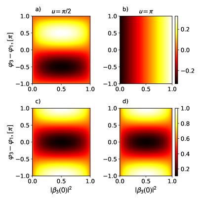
The interplay between phase and amplitude information in Eq. (14) is shown in Fig. 2, where the difference $\left|{\beta_{1}(t)}\right|^{2}-\left|{\beta_{3}(t)}\right|^{2}$ is taken in the limit $e^{-\Lambda(t)}\to 1$ . We suppress the first term by choosing $u(t)=\pi/2$ and from Fig. 2 one sees that for any initial phase difference between qubit states $\left|1\right\rangle$ and $\left|3\right\rangle$ there is a unique value of the population differences. We also note that in limit when $\left|{\beta_{3}(t)}\right|^{2}=0,1$ the measurable value equals $0$ , which becomes clear from Eq. (8) where off-diagonal elements vanish and the phases are totally uncertain.

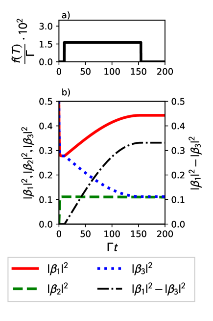
As a demonstration of our method we verified the validity of Eq. (14) by numerical simulation for initially equal probability amplitudes $|\beta_{1}(0)|=|\beta_{3}(0)|=1/\sqrt{2}$ , $\beta_{2}(0)=0$ , and $\varphi_{3}-\varphi_{1}=0.4\pi$ . In this case, the only non zero term in the right hand side of Eq. (14) is proportional to $\sin{u(t)}$ . For a $\pi/2$ modulation ( $u(t)=\pi/2$ ) the population difference at the end of the pulse is proportional to $\sin{(\varphi_{1}-\varphi_{3})}$ as it follows from (20). This behavior is shown in Fig. 3.

Alternatively, for a $\pi$ modulation pulse ( $u(t)=\pi$ ) the population difference $|\beta_{1}(t)|^{2}-|\beta_{3}(t)|^{2}$ after the end of the pulse becomes equal to zero which is shown in Fig. 4.

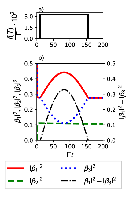
Also, it is worth mentioning that after the modulation pulse $\left|{\beta_{1}(t)}\right|^{2}+\left|{\beta_{3}(t)}\right|^{2}\neq 1$ , because the central qubit becomes partially excited. Nevertheless, we are interested only in a combination of measured populations. In summary to this section, we may conclude that modulating the frequency of the second qubit allows us to obtain the unambiguous information about the phase difference $\varphi_{1}-\varphi_{3}$ via the measurement of the evolution of the probability amplitudes $|\beta_{1}(t)|^{2}$ , $|\beta_{3}(t)|^{2}$ .

To emulate the reconstruction procedure we take the state with an unknown phase difference ${\varphi_{1}}-{\varphi_{3}}$ in range $-\pi$ to $\pi$ and with unknown populations $\beta_{1,3}$ . Then, we simulate the dynamics after the $u=\pi$ pulse and get the difference of populations $d(t_{\pi})=\left|{\beta_{1}}\right|^{2}-\left|{\beta_{3}}\right|^{2}$ . The estimation of the populations from Eq. (19) is:

\begin{gathered}\left|\beta_{1}^{est}\left(0\right)\right|=\sqrt{\frac{1}{2}\left[{1-3d\left({{t_{\pi}}}\right)}\right]},\\ \left|\beta_{3}^{est}\left(0\right)\right|=\sqrt{\frac{1}{2}\left[{1+3d\left({{t_{\pi}}}\right)}\right]}.\end{gathered}

(22)

At the next step we simulate the dynamics after a $u=\pi/2$ pulse and take the populations $\left|{\beta_{1}}\right|^{2}$ and $\left|{\beta_{3}}\right|^{2}$ after the pulse. Then, following equations Eqs. (20) and (21), where $S$ and $d(t_{\pi/2})$ are in fact the measured values, we find the $\sin$ and $\cos$ values of estimated phase $\varphi_{\rm est}$ :

\begin{gathered}\begin{array}[]{l}\sin\left({{\varphi_{est}}}\right)=\frac{3}{2}\frac{{d\left({{t_{{\pi\mathord{\left/{\vphantom{\pi 2}}\right.\kern-1.2pt}2}}}}\right)}}{{\left|{\beta_{1}^{est}\left(0\right)}\right|\left|{\beta_{3}^{est}\left(0\right)}\right|}},\\ \\ \cos\left({{\varphi_{est}}}\right)=-\left({S-\frac{5}{9}}\right)\frac{9}{{8\left|{\beta_{1}^{est}\left(0\right)}\right|\left|{\beta_{3}^{est}\left(0\right)}\right|}}\end{array}\end{gathered}

(23)

which allows to explicitly get $\varphi_{\rm est}$ through arctangent. These two steps are enough to reconstruct the state in the form Eq. (8).

IV Conclusion

In this paper we have considered three non interacting qubits embedded in an open waveguide. For this system we have described experimentally accessible method for the reconstruction within a single-excitation subspace of arbitrary two-qubit state. The method is based on the modulation of the frequency of a central ancillary qubit which allows us to determine the elements of reduced density matrix for two edge qubits.

In contrast to a common quantum tomography reconstruction where the gate pulses are applied to the measured qubits, in our method the measurement pulse is applied to the ancillary qubit. Until the projective measurements two edge qubits do not undergo any external influence.

Acknowledgements Ya. S. G. and A. A. Sh. acknowledge the support from the Ministry of Science and Higher Education of Russian Federation under grant FSUN-2020-0004.

Appendix A Derivation of the equations for the probability amplitudes $\beta_{n}(t)$

The equations for probability amplitudes $\beta_{n}(t)$ of the qubits and that of the photon $\gamma_{k}(t)$ from Eq. (4) can be found from the time-dependent Schrodinger equation $id\left|\Psi\right\rangle/dt=H\left|\Psi\right\rangle$ . For the amplitudes we obtain:

\frac{{d\beta_{1}}}{{dt}}=-i\sum\limits_{k}{}g_{k}e^{-ikd}\gamma_{k}(t)e^{-i(\omega_{k}-\Omega)t},

(24)

\frac{{d\beta_{2}}}{{dt}}=-if(t)\beta_{2}(t)-i\sum\limits_{k}{}g_{k}\gamma_{k}(t)e^{-i(\omega_{k}-\Omega)t},

(25)

\frac{{d\beta_{3}}}{{dt}}=-i\sum\limits_{k}{}g_{k}^{2}e^{ikd}\gamma_{k}(t)e^{-i(\omega_{k}-\Omega)t},

(26)

\frac{{d\gamma_{k}(t)}}{{dt}}=-ig_{k}F_{k}(t)e^{i(\omega_{k}-\Omega)t},

(27)

where

F_{k}(t)=\beta_{1}(t)e^{ikd}+\beta_{2}(t)+\beta_{3}(t)e^{-ikd}.

(28)

From (27) we obtain:

\gamma_{k}(t)=-ig_{k}\int\limits_{0}^{t}{}F_{k}(t^{\prime})e^{i(\omega_{k}-\Omega)t^{\prime}}dt^{\prime}.

(29)

The expression (29) allows us to remove the photon amplitude $\gamma_{k}(t)$ from the equations for the qubits’ amplitudes (24), (25), and (26). The result is as follows:

\begin{gathered}\frac{{d\beta_{1}}}{{dt}}=-\sum\limits_{k}{}g_{k}^{2}e^{-ikd}\int\limits_{0}^{t}{}F_{k}(t^{\prime})e^{-i(\omega_{k}-\Omega)(t-t^{\prime})}dt^{\prime},\hfill\\ \frac{{d\beta_{2}}}{{dt}}=-if(t)\beta_{2}(t)-\sum\limits_{k}{}g_{k}^{2}\int\limits_{0}^{t}{}F_{k}(t^{\prime})e^{-i(\omega_{k}-\Omega)(t-t^{\prime})}dt^{\prime},\hfill\\ \frac{{d\beta_{3}}}{{dt}}=-\sum\limits_{k}{}g_{k}^{2}e^{ikd}\int\limits_{0}^{t}{}F_{k}(t^{\prime})e^{-i(\omega_{k}-\Omega)(t-t^{\prime})}dt^{\prime},\hfill\\ \end{gathered}

(30)

In accordance with Wigner-Weiskopff approximation we take the quantity $F_{k}(t)$ out the integrands,

\begin{gathered}\frac{{d\beta_{1}}}{{dt}}=-\sum\limits_{k}{}g_{k}^{2}e^{-ikd}F_{k}(t)I_{k}(\Omega,t),\hfill\\ \frac{{d\beta_{2}}}{{dt}}=-if(t)\beta_{2}(t)-\sum\limits_{k}{}g_{k}^{2}F_{k}(t)I_{k}(\Omega,t),\hfill\\ \frac{{d\beta_{3}}}{{dt}}=-\sum\limits_{k}{}g_{k}^{2}e^{ikd}F_{k}(t)I_{k}(\Omega,t),\hfill\\ \end{gathered}

(31)

where

\begin{gathered}I_{k}(\Omega,t)=\int\limits_{0}^{t}{e^{-i(\omega_{k}-\Omega)(t-t^{\prime})}dt^{\prime}}=\int\limits_{0}^{t}{e^{-i(\omega_{k}-\Omega)\tau}d\tau}\hfill\\ \approx\int\limits_{0}^{\infty}{e^{-i(\omega_{k}-\Omega)\tau}d\tau}=\pi\delta(\omega_{k}-\Omega)-iP.v.\left({\frac{1}{{\omega_{k}-\Omega}}}\right)\hfill\\ \end{gathered}

(32)

We assume $g_{-k}=g_{k},I_{-k}(\Omega,t)=I_{k}(\Omega,t)$ and leave the summation in (31) over positive valued of $k$ (positive frequencies).

\begin{gathered}\frac{{d\beta_{1}}}{{dt}}=-\sum\limits_{k>0}{}g_{k}^{2}\left({e^{-ikd}F_{k}(t)+e^{ikd}F_{-k}(t}\right)I_{k}(\Omega,t),\hfill\\ \frac{{d\beta_{2}}}{{dt}}=-if(t)\beta_{2}(t)-\sum\limits_{k>0}{}g_{k}^{2}\left({F_{k}(t)+F_{-k}(t}\right)I_{k}(\Omega,t),\hfill\\ \frac{{d\beta_{3}}}{{dt}}=-\sum\limits_{k>0}{}g_{k}^{2}\left({e^{ikd}F_{k}(t)+e^{-ikd}F_{-k}(t}\right)I_{k}(\Omega,t).\hfill\\ \end{gathered}

(33)

Inserting the explicit form of $F_{k}(t)$ (28) in (33) results in the following expressions:

\begin{gathered}\frac{{d\beta_{1}}}{{dt}}=-2\sum\limits_{k>0}{}g_{k}^{2}\left({\beta_{1}+\beta_{2}\cos kd+\beta_{3}\cos 2kd}\right)I_{k}(\Omega,t),\hfill\\ \frac{{d\beta_{2}}}{{dt}}=-if(t)\beta_{2}(t)\hfill\\ -2\sum\limits_{k>0}{}g_{k}^{2}\left({\beta_{1}\cos kd+\beta_{2}+\beta_{3}\cos kd}\right)I_{k}(\Omega,t),\hfill\\ \frac{{d\beta_{3}}}{{dt}}=-2\sum\limits_{k>0}{}g_{k}^{2}\left({\beta_{1}\cos 2kd+\beta_{2}\cos kd+\beta_{3}}\right)I_{k}(\Omega,t).\hfill\\ \end{gathered}

(34)

The next step is to relate the coupling constants $g_{k}$ to the qubit decay rate of spontaneous emission into the waveguide mode. In accordance with Fermi golden rule we define the qubit decay rates by the following expressions:

\Gamma=2\pi\sum\limits_{k}{g_{k}^{2}\delta(\omega_{k}-\Omega)}

(35)

For the 1D case, a summation over $k$ is replaced by an integration over $\omega$ in accordance with the prescription

2\sum\limits_{k>0}{}\Rightarrow\frac{L}{{2\pi}}2\int\limits_{0}^{\infty}{d\left|k\right|}=\frac{L}{{\pi\upsilon_{g}}}\int\limits_{0}^{\infty}{d\omega_{k}},

(36)

where $L$ is a length of the waveguide, and we assumed a linear dispersion law, $\omega_{k}=v_{g}|k|$ . The application of (36) to (35), allows to derive a relation between the coupling constant $g_{k}$ and the decay rate $\Gamma$ ,

g_{k}=\left({\frac{{v_{g}\Gamma}}{{2L}}}\right)^{1/2}.

(37)

Now we can calculate the different terms in (34).

\begin{gathered}\sum\limits_{k}{g_{k}^{2}I_{k}(\Omega,t)}=\sum\limits_{k}{g_{k}^{2}}\left({\pi\delta(\omega_{k}-\Omega)-iP.v.\left({\frac{1}{{\omega_{k}-\Omega}}}\right)}\right)\hfill\\ =\frac{\Gamma}{2}-iP.v.\left({\frac{{g_{k}^{2}}}{{\omega_{k}-\Omega}}}\right)\approx\frac{\Gamma}{2},\hfill\\ \end{gathered}

(38)

\begin{gathered}2\sum\limits_{k>0}{g_{k}^{2}\cos(kd)}I_{k}(\Omega,t)\hfill\\ =\frac{L}{{\upsilon_{g}}}\int\limits_{0}^{\infty}{g_{k}^{2}\cos(kd)\delta(\omega_{k}-\Omega)d\omega_{k}}-2i\sum\limits_{k>0}{}P.v.\left({\frac{{g_{k}^{2}\cos(kd)}}{{\omega_{k}-\Omega}}}\right)\hfill\\ =\frac{L}{{\upsilon_{g}}}g_{\Omega}^{2}\cos(k_{\Omega}d)-i\frac{L}{{v_{g}\pi}}g_{\Omega}^{2}P.v.\int\limits_{0}^{\infty}{}\frac{{\cos\left({\frac{\omega}{{v_{g}}}d}\right)}}{{\omega-\Omega}}\hfill\\ \end{gathered}

(39)

For the principal value integral in (39) we obtain:

P.v.\int\limits_{0}^{\infty}{d\omega}\frac{{\cos\left({\frac{\omega}{{v_{g}}}d}\right)}}{{\omega-\Omega}}=-\pi\sin\left({k_{\Omega}d}\right)

(40)

where $k_{\Omega}=\Omega/v_{g}$ .

The expression (40) is exact if counter-rotating terms in the qubit-field interaction are taken into account (Suppl. in Gonz2013 ). Nevertheless, within a rotating wave approximation the Eq. 40 provides a good accuracy for $d>\lambda/4$ Green2021 .

2\sum\limits_{k>0}{g_{k}^{2}\cos(kd)}I_{k}(\Omega,t)=\frac{L}{{\upsilon_{g}}}g_{\Omega}^{2}e^{ik_{\Omega}d}=\frac{\Gamma}{2}e^{ik_{\Omega}d}.

(41)

Similar calculations also give for the sum in (34):

2\sum\limits_{k>0}{g_{k}^{2}\cos(2kd)}I_{k}(\Omega,t)=\frac{\Gamma}{2}e^{2ikd}.

(42)

In (38) the decay rate $\Gamma$ is defined by (35). The principal value in (38) gives rise to the shift of the qubit frequency. Therefore, we incorporate it in the renormalized qubit frequency and will not write it explicitly any more.

Collecting together (38), (41), and (42) we write the final form of the equations (34):

\begin{gathered}\frac{{d\beta_{1}}}{{dt}}=-\frac{\Gamma}{2}\left({\beta_{1}+\beta_{2}e^{ikd}+\beta_{3}e^{i2kd}}\right),\hfill\\ \frac{{d\beta_{2}}}{{dt}}=-if(t)\beta_{2}(t)-\frac{\Gamma}{2}\left({\beta_{1}e^{ikd}+\beta_{2}+\beta_{3}e^{ikd}}\right),\hfill\\ \frac{{d\beta_{3}}}{{dt}}=-\frac{\Gamma}{2}\left({\beta_{1}e^{i2kd}+\beta_{2}e^{ikd}+\beta_{3}}\right),\hfill\\ \end{gathered}

(43)

Appendix B Derivation of equation (14)

Equations (5) can be written in the matrix form:

\frac{d\widehat{\beta}}{dt}=A(t)\widehat{\beta}(t),

(44)

where

{\widehat{\beta}(t){=}}\left({\begin{array}[]{*{20}c}{\beta_{1}(t)}\\ {\beta_{2}}(t)\\ {\beta_{3}(t)}\\ \end{array}}\right),

(45)

{\text{A(t) = }}-\frac{\Gamma}{2}\left({\begin{array}[]{*{20}c}1&{e^{ikd}}&{e^{2ikd}}\\ {e^{ikd}}&{1+if(t)\frac{2}{\Gamma}}&{e^{ikd}}\\ {e^{2ikd}}&{e^{ikd}}&1\\ \end{array}}\right).

(46)

It is easy to verify that the matrices $A(t)$ do not commute at different times $[A(t_{1}),A(t_{2})]\neq 0$ . In this case the solution of (44) can be obtained in the form:

\widehat{\beta}(t)=e^{M(t)}\widehat{\beta}(0)

(47)

where the Magnus operator $M(t)$ can be written as infinite series expansion Blanes2009 :

M(t)=\sum\limits_{n=1}^{\infty}{M_{n}}(t).

(48)

The first two terms in (48) are as follows:

\begin{gathered}M_{1}(t)=\int\limits_{0}^{t}{dt_{1}A(t_{1})},\hfill\\ M_{2}(t)=\frac{1}{2}\int\limits_{0}^{t}{dt_{2}\int\limits_{0}^{t_{2}}{dt_{1}}\left[{A(t_{1})A(t_{2})}\right]}.\hfill\\ \end{gathered}

(49)

According to Silvester’s matrix theorem (named after J. J. Sylvester) any analytic function $z(M)$ of a quadratic $n\times n$ matrix $M$ can be expressed as a polynomial in $M$ , in terms of the eigenvalues and eigenvectors of $M$ Horn1991 . Specifically, the theorem states that

z(M)=\sum\limits_{i=1}^{n}{z(\lambda_{i})B_{i}},

(50)

where $\lambda_{i}$ are the characteristic roots of the equation

\det\left|{M-\lambda I}\right|=0,

(51)

and

B_{i}=\prod\limits_{j=1,i\neq j}^{n}{\frac{{M-\lambda_{j}I}}{{\lambda_{i}-\lambda_{j}}}},

(52)

where $I$ is the identity matrix.

The Silvester’s formula (50) holds for any quadratic diagonalizable matrix all roots of which are different.

In the sum of (48) we neglect all terms except for the first one, $M(t)=M_{1}(t)$ :

M_{1}(t)=\int\limits_{0}^{t}{dt_{1}A(t_{1})}{\text{ = }}-\frac{{\Gamma t}}{2}\left({\begin{array}[]{*{20}c}1&{e^{ikd}}&{e^{2ikd}}\\ {e^{ikd}}&{\Omega(t)}&{e^{ikd}}\\ {e^{2ikd}}&{e^{ikd}}&1\\ \end{array}}\right),

(53)

where

\Omega(t)=1+i\frac{2}{{\Gamma t}}\int\limits_{0}^{t}{f(t_{1})dt_{1}}=1-\frac{2}{{\Gamma t}}F(t),

(54)

F(t)=-i\int\limits_{0}^{t}{f(t_{1})dt_{1}}.

(55)

Next, we find the characteristic roots $\lambda_{i}(t)$ of the matrix $M_{1}(t)$ , which are the roots of the equation

\det\left|{M_{1}(t)-\lambda(t)I}\right|=0.

(56)

The equation (56) is a cubic equation

\left({1-\lambda}\right)^{2}\left({\Omega-\lambda}\right)+2e^{4ikd}-e^{4ikd}\left({\Omega-\lambda}\right)-2e^{2ikd}\left({1-\lambda}\right)=0,

(57)

with the following three roots

\begin{gathered}\lambda_{1,2}(t)=-\frac{{\Gamma t}}{2}\left({1+\frac{1}{2}e^{2ikd}}\right)+\frac{1}{2}F(t)\hfill\\ \pm\frac{1}{4}e^{ikd}\sqrt{\left({8+e^{2ikd}}\right)\Gamma^{2}t^{2}+4F^{2}(t)e^{-2ikd}+4F(t)\Gamma t},\hfill\\ \end{gathered}

(58)

\lambda_{3}(t)=\frac{{\Gamma t}}{2}\left({e^{2ikd}-1}\right).

(59)

In the equation (58) the roots $\lambda_{1}$ , $\lambda_{2}$ correspond to $+$ , $-$ sign, respectively.

The application of 50 to $z(M)=e^{M}$ gives rise to the following equation:

e^{M_{1}(t)}=B_{1}e^{\lambda_{1}}+B_{2}e^{\lambda_{2}}+B_{3}e^{\lambda_{3}},

(60)

where

\begin{gathered}B_{1}=\left({\frac{{M_{1}-\lambda_{2}I}}{{\lambda_{1}-\lambda_{2}}}}\right)\left({\frac{{M_{1}-\lambda_{3}I}}{{\lambda_{1}-\lambda_{3}}}}\right)\hfill\\ \quad=\frac{{M_{1}^{2}-(\lambda_{2}+\lambda_{3})M_{1}+\lambda_{2}\lambda_{3}I}}{{(\lambda_{1}-\lambda_{2})(\lambda_{1}-\lambda_{3})}},\hfill\\ \end{gathered}

(61)

\begin{gathered}B_{2}=\left({\frac{{M_{1}-\lambda_{1}I}}{{\lambda_{2}-\lambda_{1}}}}\right)\left({\frac{{M_{1}-\lambda_{3}I}}{{\lambda_{2}-\lambda_{3}}}}\right)\hfill\\ \quad=\frac{{M_{1}^{2}-(\lambda_{1}+\lambda_{3})M_{1}+\lambda_{1}\lambda_{3}I}}{{(\lambda_{2}-\lambda_{1})(\lambda_{2}-\lambda_{3})}},\hfill\\ \end{gathered}

(62)

\begin{gathered}B_{3}=\left({\frac{{M_{1}-\lambda_{1}I}}{{\lambda_{3}-\lambda_{1}}}}\right)\left({\frac{{M_{1}-\lambda_{2}I}}{{\lambda_{3}-\lambda_{2}}}}\right)\hfill\\ \quad=\frac{{M_{1}^{2}-(\lambda_{1}+\lambda_{2})M_{1}+\lambda_{2}\lambda_{1}I}}{{(\lambda_{3}-\lambda_{1})(\lambda_{3}-\lambda_{2})}}.\hfill\\ \end{gathered}

(63)

The equations (60)-(63) are valid for any value of $kd$ .

Below we assume $kd=\pi n$ , where $n$ is a positive integer. For this case $\lambda_{3}=0$ and we obtain

e^{M_{1}(t)}=B_{1}e^{\lambda_{1}}+B_{2}e^{\lambda_{2}}+B_{3},

(64)

\begin{gathered}B_{1}=\frac{{M_{1}^{2}-\lambda_{2}M_{1}}}{{(\lambda_{1}-\lambda_{2})\lambda_{1}}},\hfill\\ B_{2}=\frac{{M_{1}^{2}-\lambda_{1}M_{1}}}{{(\lambda_{2}-\lambda_{1})\lambda_{2}}},\hfill\\ B_{3}=\frac{{M_{1}^{2}-(\lambda_{1}+\lambda_{2})M_{1}}}{{\lambda_{1}\lambda_{2}}}+I,\hfill\\ \end{gathered}

(65)

where

\begin{gathered}\lambda_{1,2}(t)=-\frac{{3\Gamma t}}{4}+\frac{1}{2}F(t)\hfill\\ \quad\quad\pm(-1)^{n}\frac{1}{4}\sqrt{9\Gamma^{2}t^{2}+4F^{2}(t)+4F(t)\Gamma t}.\hfill\\ \end{gathered}

(66)

Below we perform the calculations for $kd=2\pi$ . Using the equation (47) and the explicit expression (53) for the matrix $M_{1}(t)$ we obtain from (64), (65), (66) the expressions for qubits amplitudes $\beta_{1}(t)$ , $\beta_{3}(t)$ .

\beta_{1}(t,2\pi)=\frac{{\Gamma t}}{R}\left({\beta_{1}(0)+\beta_{3}(0)}\right)\left({\frac{{\left({\frac{{3\Gamma t}}{2}+F-\frac{R}{2}}\right)}}{{\left({-\frac{{3\Gamma t}}{2}+F+\frac{1}{2}R}\right)}}e^{\lambda_{1}}-\frac{{\left({\frac{3}{2}\Gamma t+F+\frac{R}{2}}\right)}}{{\left({-\frac{{3\Gamma t}}{2}+F-\frac{1}{2}R}\right)}}e^{\lambda_{2}}}\right)+\frac{1}{2}\left({\beta_{1}(0)-\beta_{3}(0)}\right),

(67)

\beta_{3}(t,2\pi)=\frac{{\Gamma t}}{R}\left({\beta_{1}(0)+\beta_{3}(0)}\right)\left({\frac{{\left({\frac{{3\Gamma t}}{2}+F-\frac{R}{2}}\right)}}{{\left({-\frac{{3\Gamma t}}{2}+F+\frac{1}{2}R}\right)}}e^{\lambda_{1}}-\frac{{\left({\frac{3}{2}\Gamma t+F+\frac{R}{2}}\right)}}{{\left({-\frac{{3\Gamma t}}{2}+F-\frac{1}{2}R}\right)}}e^{\lambda_{2}}}\right)-\frac{1}{2}\left({\beta_{1}(0)-\beta_{3}(0)}\right),

(68)

where

R=\sqrt{9\Gamma^{2}t^{2}+4F^{2}(t)+4F(t)\Gamma t}.

(69)

Now we analyze the quantities $R$ , $\lambda_{1}$ , $\lambda_{2}$ for $\Gamma t\gg|F|$ . We obtain

R\approx 3\Gamma t+\frac{2}{3}F+\frac{{16}}{{27}}\frac{{F^{2}}}{{\Gamma t}},

(70)

\lambda_{1}(t)=-\frac{{3\Gamma t}}{4}+\frac{1}{2}F(t)+\frac{1}{4}R\approx\frac{2}{3}F+\frac{4}{{27}}\frac{{F^{2}}}{{\Gamma t}},

(71)

\lambda_{2}(t)=-\frac{{3\Gamma t}}{4}+\frac{1}{2}F(t)-\frac{1}{4}R\approx-\frac{3}{2}\Gamma t+\frac{1}{3}F-\frac{4}{{27}}\frac{{F^{2}}}{{\Gamma t}}.

(72)

Therefore, in (67), (68) we neglect the decaying exponent $e^{\lambda_{2}}\approx e^{-\frac{3}{2}\Gamma t}$ . The quantity $e^{\lambda_{1}}$ we write in the following form:

e^{\lambda_{1}}\approx\exp\left({\frac{2}{3}F+\frac{4}{{27}}\frac{{F^{2}}}{{\Gamma t}}}\right)\equiv e^{-iu(t)}e^{-\Lambda(t)},

(73)

where

u(t)=\frac{2}{3}\int\limits_{0}^{t}{f(\tau)d\tau},

(74)

\Lambda(t)=\frac{4}{{27\Gamma t}}\left({\int\limits_{0}^{t}{f(\tau)d\tau}}\right)^{2}.

(75)

For this approximation the equations (67), (68) take the form:

\begin{gathered}\beta_{1}(t,2\pi)=\frac{1}{6}\left({\beta_{1}(0)+\beta_{3}(0)}\right)e^{-iu(t)}e^{-\Lambda(t)}\hfill\\ +\frac{1}{2}\left({\beta_{1}(0)-\beta_{3}(0)}\right),\hfill\\ \end{gathered}

(76)

\begin{gathered}\beta_{3}(t,2\pi)=\frac{1}{6}\left({\beta_{1}(0)+\beta_{3}(0)}\right)e^{-iu(t)}e^{-\Lambda(t)}\hfill\\ -\frac{1}{2}\left({\beta_{1}(0)-\beta_{3}(0)}\right),\hfill\\ \end{gathered}

(77)

\beta_{2}(t)=-\frac{{\left({\beta_{1}(0)+\beta_{3}(0)}\right)}}{3}e^{-iu(t)}e^{-\Lambda(t)}.

(78)

From (76), (77) we finally obtain for $kd=2\pi$

\begin{gathered}\left|{\beta_{1}(t)}\right|^{2}-\left|{\beta_{3}(t)}\right|^{2}=\frac{1}{3}\left({\left|{\beta_{1}(0)}\right|^{2}-\left|{\beta_{3}(0)}\right|^{2}}\right)e^{-\Lambda(t)}\cos u(t)\hfill\\ -\frac{1}{3}i\left({\beta_{1}^{*}(0)\beta_{3}(0)-\beta_{1}(0)\beta_{3}^{*}}\right)e^{-\Lambda(t)}\sin u(t),\hfill\\ \end{gathered}

(79)

\begin{gathered}\left|{\beta_{1}(t)}\right|^{2}+\left|{\beta_{3}(t)}\right|^{2}=\frac{1}{{18}}\left({e^{-\Lambda(t)}+9}\right)\hfill\\ +\frac{1}{9}\left({\beta_{1}^{*}(0)\beta_{3}(0)+\beta_{1}(0)\beta_{3}^{*}}\right)\left({e^{-\Lambda(t)}-9}\right),\hfill\\ \end{gathered}

(80)

\left|{\beta_{2}(t)}\right|^{2}=\frac{1}{9}e^{-2\Lambda(t)}\left({1+2\left|{\beta_{1}(0}\right|\left|{\beta_{3}(0)}\right|\cos\left({\varphi_{1}-\varphi_{3}}\right)}.\right)

(81)

which are the equations (14), (19), (16) from the main text.

References

(1) E.Toninelli, B. Ndagano, A. Valles et. al. Concepts in quantum state tomography and classical implementation with intense light: a tutorial, Adv. Opt. Photonics Vol.11, No. 1 ,344254 (2019)
(2) R.Schmied, Quantum state tomography of a single qubit: comparison of methods, J. Mod. Opt., Vol.63, pp.1744-1758 (2016)
(3) A. Blais, R. S. Huang, A. Wallraff, S. M. Girvin, and R. J.Schoelkopf, Cavity quantum electrodynamics for superconducting electrical circuits: An architecture for quantum computation, Phys. Rev. A 69,062320 (2004).
(4) M. Steffen, M.Ansmann, R.McDermott et.al. State tomography of capacitively shunted phase qubits with high fidelity, Phys. Rev. Lett. 97,050502 (2006).
(5) M. Steffen, M.Ansmann, R.C. Bialczak et.al. Measurement of the entanglement of two superconducting qubits via state tomography, Sci. Rep., Vol. 13 Iss. 5792, pp. 1423-1425 (2006)
(6) J. D. Brehm, A. N. Poddubny, A. Stehli, Tim Wolz, H. Rotzinger and A. V. Ustinov, Waveguide bandgap engineering with an array of superconducting qubits, npj Quantum Mater., 6, 10(2021)
(7) Forn-Díaz, P., García-Ripoll, J., Peropadre, B. et al. Ultrastrong coupling of a single artificial atom to an electromagnetic continuum in the nonperturbative regime. Nature Phys 13, 39–43 (2017).
(8) K. Koshino, H. Terai, K. Inomata, T. Yamamoto, W. Qiu, Z. Wang, and Y. Nakamura, Observation of the Three-State Dressed States in Circuit Quantum Electrodynamics, Phys. Rev. Lett. 110, 263601 (2013)
(9) Mirhosseini, M., Kim, E., Zhang, X. et al. Cavity quantum electrodynamics with atom-like mirrors. Nature 569, 692–697 (2019).
(10) D. Kornovan et. al.,Doubly excited states in a chiral waveguide-QED system: description and properties, J. Phys.: Conf. Ser. 2015 012070 (2021)
(11) Fang, YL.L., Zheng, H. Baranger, H.U. One-dimensional waveguide coupled to multiple qubits: photon-photon correlations. EPJ Quantum Technol. 1, 3 (2014).
(12) Y.-L. L. Fang, Harold U. Baranger, Waveguide QED: Power spectra and correlations of two photons scattered off multiple distant qubits and a mirror Phys. Rev. A 91, 053845 (2015)
(13) I. Issah, H. Caglayan, Qubit–qubit entanglement mediated by epsilon-near-zero waveguide reservoirs, Appl. Phys. Lett. 119, 221103 (2021);
(14) A. F. Kockum, G. Johansson and F. Nori, Decoherence-Free Interaction between Giant Atoms in Waveguide Quantum Electrodynamics, Phys. Rev. Lett. 120, 140404 (2018)
(15) A. Albrecht, L. Henriet, A. Asenjo-Garcia, P. B. Dieterle, O. Painter and D. E. Chang, Subradiant states of quantum bits coupled to a one-dimensional waveguide, New J. Phys. 21 025003 (2019)
(16) Ya. S. Greenberg, A. N. Sultanov, Influence of the nonradiative decay of qubits into a common channel on the transport properties of microwave photons, JETP Letters 106,406-410 (2017)
(17) A.N. Sultanov, Ya. S. Greenberg, Transfer of excited state between two qubits in an open waveguide, Low Temperature Physics 44, 203 (2018)
(18) Y. P. Zhong, H.S. Chang, K. J. Satzinger et. al Violating Bell’s inequality with remotely connected superconducting qubits, Nat. Phys. 15, 741-744 (2019)
(19) Ya. S. Greenber, A. A. Shtygashev, Non-Hermitian Hamiltonian approach to the microwave transmission through a one-dimensional qubit chain, Phys. Rev. A 92, 063835 (2015)
(20) A.F. van Loo, A. Fedorov, K. Laluniere et. al. Photon-mediated interactions between distant artificial atoms, Science 342, 1494 (2013)
(21) M. Cattaneo, G. L. Giorgi, S. Maniscalco, G. S. Paraoanu, and R. Zambrini, Ann. Phys. (Berlin) 533, 2100038 (2021)
(22) P.Y. Wen, K.T. Lin, A. F. Kockum et.al. Large Collective Lamb Shift of Two Distant Superconducting Artificial Atoms, Phys. Rev. Lett. 123, 233602 (2019)
(23) M. P. Silveri, J. A. Tuorila, E. V. Thuneberg, and G. S. Paraoanu, Quantum systems under frequency modulation, Rep. Prog. Phys. 80, 056002 (2017).
(24) A. Gonzalez-Tudela and D. Porras, Mesoscopic Entanglement Induced by Spontaneous Emission in Solid-State Quantum Optics, Phys. Rev. Lett. 110, 080502 (2013).
(25) Ya. S. Greenberg, A. A. Shtygashev, and A. G. Moiseev, Spontaneous decay of artificial atoms in a three-qubit system. Eur. Phys. J. B94, 221 (2021).
(26) S. Blanes, F. Casas, J.A. Oteo, and J. Ros, The Magnus expansion and some of its applications. Physics Reports 470, 151 (2009).
(27) R. A. Horn and Ch. R. Johnson Topics in Matrix Analysis. Cambridge University Press, 1991.

Quantum phase measurement of two-qubit states in an open waveguide

Abstract

I Introduction

II Formulation of the problem

III Tomography of the two-qubit state

III.1 Free evolution of the three-qubit system

III.2 Measurement of the phase difference by frequency modulation

IV Conclusion

Appendix A Derivation of the equations for the probability amplitudes βn​(t)\beta_{n}(t)

Appendix B Derivation of equation (14)

References

Appendix A Derivation of the equations for the probability amplitudes $\beta_{n}(t)$