Quantum Monte Carlo sign bounds, topological Mott insulator and thermodynamic transitions in twisted bilayer graphene model

Although the sign problem often implies exponential computational complexity, it is worthwhile to emphasize that not all sign problems cause such severe damage. Very recently, a much more mild type of sign problem has been demonstrated, where the computation complexity scales as a polynomial function of the system size, known as polynomial sign problem [58, 59].

In this Letter, we study the sign problem in TBG flat bands. Utilizing the sign bound theory [60], we prove that TBG flat bands at even integer fillings, or arbitrary integer fillings in the chiral limit, exhibit (at most) polynomial sign problem. This observation allows us to utilize QMC methods to study fillings away from charge neutrality, away from the chiral limit, and/or in the presence of extra attractive interactions on top of the Coulomb repulsion (See Tab. 1 for details).

To demonstrate this new approach, we performed large-scale QMC simulations to examine the chiral limit at filing $\nu=1$ (we denote the fully empty/filled flat bands as $\nu=-4/+4$ and charge neutrality as $\nu=0$). At $T=0$, this model can be solved exactly [51, 53, 56], and the exact solution reveals that at $T\to 0$, the system is a correlated Chern insulator – a topological Mott insulator (TMI) [61, 62, 63, 64, 65, 66] – with Chern number $C=1$. Upon raising the temperature, the insulating state shall “melt” into a metal and the time-reversal symmetry shall be recovered. However, our knowledge about this finite-temperature phase transition is very limited. Because the sign problem is only polynomial, QMC simulations become a highly efficient tool to study this system, from which three different phases/states are observed (1) a metal phase with time-reversal symmetry at high temperature $T>T^{\star}$, (2) a time-reversal invariant pseudo-gap phase at intermediate temperature $T_{c}<T<T^{\star}$ and (3) a low-temperature TMI phase at $T<T_{c}$. Here, $T^{\star}$ is a crossover temperature scale and $T_{c}$ is the critical temperature of a second order phase transition, at which the time-reversal symmetry is spontaneously broken. We further show that the TMI phase only breaks the time reversal symmetry, while spins remain disordered due to thermal excitations of gapless spin fluctuations. This absence of spin order/polarization is in direct contrast to quantum Hall states where electron spins are polarized due to Zeeman splitting and thus spin fluctuations are gapped. In the discussion section, we establish the connection and consistency between our simulations and recent experimental studies on TMI phases in $h$-BN nonaligned TBG devices [41].

For interactions, in addition to the Coulomb repulsion, here we have the option to include one more interaction term and the sign problem will still remain polynomial.

The first term in $H_{I}$ ($V_{1}>0$) is the Coulomb interactions, and the second term $V_{2}\geq 0$ introduces repulsive interactions for fermions in the same valley and attractions between the two valleys, which can be introduced as a phenomenology term describing inter-valley attractions [68, 69, 70, 71, 72]. At $V_{2}=0$, this model recovers the standard TBG model with Coulomb repulsions. When $V_{2}$ is turned on, the inter-valley attraction favors inter-valley pairing and could stabilize a superconducting ground state. The normalization factor in $H_{I}$ is $\Omega=L^{2}\frac{\sqrt{3}}{2}a_{M}^{2}$ with $L$ being the linear system size of the system. $\mathbf{k}$ and $\mathbf{q}$ cover the whole momentum space, $\nu$ is the filling factor and $\alpha,\tau,s$ represent layer/sublattice, valley, spin indices, respectively. The mometum dependence for non-negative $V_{1}$ and $V_{2}$ is unimportant to polynomial sign problem. Here, for simplicity, we set $V_{2}=\gamma V_{1}$ with $\gamma$ being a non-negative constant and for $V_{1}$, we use Coulomb interaction screened by single gate in our simulation $V_{1}({\mathbf{q}})=\frac{e^{2}}{4\pi\varepsilon}\int d^{2}{\mathbf{r}}\left(\frac{1}{{\mathbf{r}}}-\frac{1}{\sqrt{{\mathbf{r}}^{2}+d^{2}}}\right)e^{i{\mathbf{q}}\cdot{\mathbf{r}}}=\frac{e^{2}}{2\varepsilon}\frac{1}{\left|{\mathbf{q}}\right|}\left(1-e^{-\left|{\mathbf{q}}\right|d}\right)$ where $\frac{d}{2}=20\,\mathrm{nm}$ is the distance between graphene layer and single gate, $\epsilon=7\epsilon_{0}$ is the dielectric constant. We then project the interactions $H_{I}$ to the moiré flat bands (See SM [73]) and use the projected Hamiltonian to carry out sign bounds analysis and QMC simulations.

It is worthwhile to emphasize that the sign problem doesn’t always lead to an exponentially high computational cost. To measure the severity of the sign problem, here we use the average sign $\left\langle sign\right\rangle=\sum_{l}W_{l}/\sum_{l}|Re(W_{l})|$, where $|Re(W_{l})|$ is the absolute value of the real part of $W_{l}$. For physical partition function $Z=\sum_{l}W_{l}=\sum_{l}Re(W_{l})$, this average sign is between $0$ and $1$, and $\left\langle sign\right\rangle=1$ means that the system is sign problem free, while smaller $\left\langle sign\right\rangle$ means severer sign problem. In a $d$-dimension quantum systems that suffers from the sign problem, $\left\langle sign\right\rangle\sim\exp(-\beta L^{d})$ where $\beta=1/T$ the inverse temperature, indicating that the number of configurations needed in QMC simulations scales as an exponential function of the space-time volume. For polynomial sign problem, although $\left\langle sign\right\rangle<1$ (i.e., the system does suffer from the sign problem), $1/\left\langle sign\right\rangle$ is a polynomial function of the system size, and thus the number of configurations needed only scales as a power-law function of the system size.

Although the average sign can be easily measured in QMC simulations, it usually doesn’t have a simple analytic formula. To estimate the numerical cost to overcome the sign problem, we utilize the sign bound $\left\langle sign\right\rangle_{b}$ defined in Ref. [60]. As proved in Ref. [60], $\left\langle sign\right\rangle_{b}$ is the lower bound of $\left\langle sign\right\rangle$ (i.e., $\left\langle sign\right\rangle_{b}\leqslant\left\langle sign\right\rangle$). Thus, if the sign bound scale is a power-law function of the system size, the sign problem is (at most) polynomial. Remarkably, the low temperature sign bound in moiré flat bands can be easily calculated by counting ground state degeneracy, which can be obtained using SU(4) and SU(2) Young diagram as employed in Refs. [50, 51, 56] (See SM for details [73]).

Details about this calculation are shown in the SM and the conclusions are summarized in Tab. 1. At charge neutrality ($\nu=0$), moiré flat bands with Coulomb interactions ($\gamma=0$) is known to be sign problem free [55, 56], and thus the sign bound is $1$. Here, we further prove that adding inter-valley attractions ($\gamma>0$) to the chiral system doesn’t cause sign problem either ($\left\langle sign\right\rangle_{b}=1$). Away from charge neutrality, sign problem arises, but it is polynomial at certain integer fillings. For Coulomb repulsion ($\gamma=0$), the sign problem is polynomial at any (even) integer fillings at (away from) the chiral limit. When inter-valley attractions are introduced ($\gamma>0$), even integer fillings at the chiral limit also have polynomial sign bound.

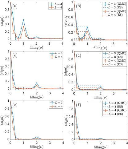
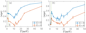
To further verify the polynomial sign problem summarized in Tab. 1, we directly calculate $\langle sign\rangle$ and $\langle sign\rangle_{b}$ in QMC simulations at various filling $\nu$, and compare them with the exact formula of the sign bound obtained at integer fillings. As shown in Fig. 1, $\langle sign\rangle$ is always larger or equal to $\langle sign\rangle_{b}$ as expected, and the sign bound at integer filling indeed converges to the exact solution. The peak in $\langle sign\rangle$ at integer (or even integer) fillings indicates that the sign problem is less severe and QMC simulations have a faster convergence at these fillings. The location of these peaks are fully consistent with the polynomial sign problem summarized in Tab. 1. The only exceptions are $\nu=3$ and $4$ of Fig. 1(a), where the sign problem is polynomial but the figure doesn’t exhibit visible peaks. This is because the power-law function here has high powers $N^{-5}$ and $N^{-8}$, which requires higher resolution (longer simulation time) to show clear distinction from exponential functions.

At low temperature limit for $\nu=1$, exact solution at $T=0$ expects degenerate ground states with Chern number $C=\pm 1$, and $\pm 3$ [51, 53, 56]. In the large system size limit $N\to\infty$, the number of ground states scales as $\propto N^{7}$ for $C=\pm 1$ and $N^{3}$ for $C=\pm 3$ [73]. Due to the higher number of ground state degeneracy, thermal fluctuations shall stabilize the $C=\pm 1$ state as the thermal equilibrium state at low temperature via the order by disorder mechanism [75]. This low-temperature state breaks spontaneously the time-reversal symmetry, but this symmetry breaking process as a function of temperature is unknown.

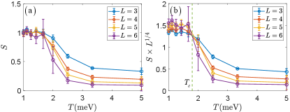
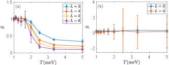
Our QMC simulation at finite temperature reveals this process. To probe the time-reversal symmetry breaking, we use the Chern band polarization as the order parameter, $\langle\hat{N}_{+}-\hat{N}_{-}\rangle/N$, where $\hat{N}_{\pm}$ are the fermion occupation number operators of $\pm$ Chern bands. The correlation function of this order parameter is plotted in Fig. 2, $S\equiv\langle(\hat{N}_{+}-\hat{N}_{-})^{2}\rangle/N^{2}$, and scaling analysis reveals a second order phase transition at $T_{c}\sim 1.8$ meV, below which the time-reversal symmetry is spontaneously broken, similar to what was observed at $\nu=3$ with real-space effective models [62, 63, 59]. At low temperature, $S$ approaches $1$, indicating that the Chern number is $C=\pm 1$, instead of $\pm 3$. In Fig. 2(b), we rescale the $y$ axis as $S\times L^{2\beta/\nu}$ using the 2D Ising exponents $\beta=1/8$ and $\nu=1$, and the cross point at $T_{c}\sim 1.8$ meV marks the critical temperature.

Such a spontaneously generated Chern insulator is of both theoretical and experimental interesting as in the temperature range of $0<T<T_{c}$, it only breaks the time reversal symmetry but not the spin-valley U(4) continuous symmetry. In contrast to quantum Hall states, where fermion spins are polarized due to Zeeman splitting, spin degrees of freedom doesn’t form any order in this TMI phase and the spin SU(2) symmetry is preserved. To better demonstrate this point, we follow the method in Ref. [52] and analytically compute the spectrum of single-particle and charge-neutral excitonic excitations at $T=0$. As shown in Fig. 3(a), single particle excitations (red stars) are fully gaped, indicating an insulating state. To restore the time-reversal symmetry, it requires to move fermions from + Chern bands to - Chern bands (or vice versa). However, such particle-hole excitations are fully gapped (yellow stars in Fig. 3(a)), and thus thermal fluctuations at low $T$ cannot restore the time-reversal symmetry. In contrast, particle-hole excitations between spin-valley bands with the same Chern number (blue starts) are gapless. These excitons describe spin SU(2) and spin-valley SU(4) fluctuations, and any spin or spin-valley order would be destroyed by these gapless excitations at any finite temperature.

We note that the energy scale of single particle gap is larger than the gap of time-reversal-restoring excitons [Fig. 3(a)], indicating that time-reversal symmetry breaking is probably more vulnerable to thermal fluctuations in comparison to single particle excitations. To probe this physics, we employ the stochastic analytic continuation (SAC) method upon the QMC imaginary time data of the Green’s function to extract the real-frequency single-particle spectra [76, 77, 78, 79]. Such QMC+SAC scheme has been successfully employed in many quantum many-body systems [80, 81, 82, 83, 84] including TBG and other moiré systems [55, 57, 71] and compared well with exact solutions and various spectroscopic experiments [78, 85, 86, 87, 88].

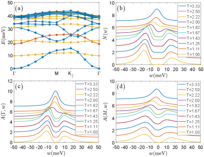
The obtained local density of states (LDOS) $N(\omega)$ and the single particle spectral functions $A(\Gamma,\omega)$ and $A(M,\omega)$ are shown in Fig. 3(b-d), respectively. From them, one sees that slightly above the $T_{c}=1.8$ meV, at $T^{\star}=2$ meV, the spectra indeed develop a pseudogap shape at both momenta and $N(\omega)$. Below $T_{c}$, the spectra are fully gapped and the system is an interaction-driven topological Mott insulator [61, 62, 63] with no spin polarization and Chern number $C=1$. The pseudogap behavior at $T_{c}<T<T^{\star}$, is certainly beyond mean-field description of the system, which would require the gap opens exactly at the transition, and is the manifestation of the intricate competition between the single-particle, collective excitations (such as the excitons) and thermal fluctuations in the morie system. Our LDOS results at low temperature with the asymmetric spectral weights, are also consistent with STM experiment at $\nu=1$ [11].

This new approach allows us to unbiasedly compute the physical properties of the model at finite temperature. For $\nu=1$, the numerical results are fully consistent with experimental observations, including spontaneous time-reversal symmetry breaking, Chern number $C=1$, and the asymmetric in LDOS. For $T_{c}<T<T^{\star}$, the simulation reveals a pseudo gap phase. This result is consistent with the observation of insulating-like behavior at $T>T_{c}$  [11]. This pseudo gap phase would be an interesting subject for further experimental studies, which will help us better understand the phase transition and mechanism that drives the time-reversal symmetry breaking in moiré flat bands.