Quantum Heat Transformers
Abstract
We propose a quantum heat transformer (QHT) designed to function analogous to classical voltage transformers. Unlike the classical counterparts, which regulate voltage, a QHT regulates temperature differences between its terminals. We initially design the device for a three-qubit system, representing the smallest possible self-contained heat transformer model. Subsequently we extend to four-qubit systems, with a specific emphasis on exploring the step-down mode for identifying the primary figure of merit. We showcase the versatility and adaptability of the models by demonstrating the availability of various self-contained setups. A key performance indicator, the capacity of thermal control, is defined to measure the capability of QHTs. An important effect in this study is the proof of existence of a necessarily transient step-down quantum heat transformer, that has a dual-mode characteristic, wherein the desired step-down mode can be realized within the transient regime of an originally designed step-up mode of the QHT. We also investigate how to control this transient domain up to which the necessarily transient mode can be achieved, by regulating the initial temperature of the qubits in the four-qubit settings. Therefore, this quantum heat transformer model not only acts as an analog to the classical voltage transformer, but also enjoys advanced characteristics, enabling it to function in both step-up and step-down modes within the same setup, unattainable for voltage transformers.
I Introduction
In this era of rapid technological advancement, the introduction of quantum devices turn out as a significant milestone in the evolution of modern technology. These groundbreaking devices harness the principles of quantum mechanics to unlock unprecedented capabilities, promising to reshape industries and revolutionize everyday life. Unlike traditional electronic devices governed by classical physics, quantum devices operate on the principles of quantum mechanics, where particles can exist in superposition of multiple states and become entangled with one another. This unique behavior enables quantum devices to perform computations, communications, and sensing tasks with efficiency and speed qualitatively higher than their classical counterparts. Examples of such quantum devices include quantum batteries [1, 2, 3], quantum heat engines [4, 5, 6], quantum refrigerators [7, 4, 8, 9, 5, 6], quantum diodes [10], quantum switches [11, 12, 13], quantum thermal transistors [14, 15, 16, 17], quantum sensors [18, 19, 20, 21], quantum thermometers [22, 23, 24], etc. Among these, quantum refrigerators, quantum heat engines, quantum thermal transistors, and quantum thermometers emerge as pivotal examples of quantum thermal devices, each promising to revolutionize thermal management at the smallest scales. In this paper, we introduce a novel thermal device: quantum heat transformers. We aim to explore the significance and potential of quantum transformers, delving into their underlying principles, design considerations, and potential applications.
An electrical transformer is a crucial device in power distribution, designed to transfer electrical energy efficiently between circuits through electromagnetic induction [25, 26, 27]. The fundamental purpose of an electric transformer is to regulate voltage levels for efficient electricity transmission. When an alternating current (AC) flows through the primary coil, it produces a changing magnetic field in the transformer’s core. This changing magnetic field induces a voltage in the secondary coil through electromagnetic induction. The resulting voltage in the secondary coil is proportional to the ratio of number of turns in secondary coil and primary coil, enabling the transformer to step up or step down the input voltage as needed for efficient power distribution. Transformers are widely used in electronics devices for voltage regulation, impedance matching, and power distribution. They play a vital role in adapting electrical energy to meet the specific requirements of various components within electronic circuits. In the realm of electronics, both step-up and step-down transformers are indispensable components, each serving critical functions tailored to specific applications. Nevertheless, step-down transformers find more frequent application and widespread use in various electronic circuits and everyday electronic devices, because when the voltage in the secondary coil is lower than that in the primary coil, it serves to reduce the input voltage to a more manageable level for electronic components.
In this paper, we present a protocol for a quantum heat transformer (QHT), drawing an analogy to the classical transformer model. Unlike classical transformers that regulate voltage, a QHT operates through temperature adjustment between two terminals. We first design a three-qubit QHT model, representing the smallest possible quantum heat transformer, and subsequently extend our investigation to four-qubit quantum heat transformers. These QHT models are self-contained, meaning they can operate without the need for any external energy sources. Similar to classical transformers, QHTs comprise two thermal junctions, each consisting of two qubits. The temperature difference between these qubits is the focus of our study. We label these two thermal junctions as the “primary thermal junction” and “secondary thermal junction”, akin to the primary and secondary coils of a classical transformer, respectively. In our QHT protocol, we initially assign a temperature to each qubit and subsequently, through interaction, analogous to electromagnetic induction, each qubit undergoes evolution, leading to the generation of new temperature differences at both the primary and secondary junctions at each evolved time step. In classical transformer the voltage difference that a transformer can increase or decrease in the secondary coil is determined by its turns ratio. In the QHT protocol, the nature of the interaction and the initial assigned temperature of the qubits allows us not only to achieve step-up or step-down transformations but also to finely regulate the capacity of thermal control (). Specifically, our investigation centers on the step-down quantum heat transformer configuration, where a step-down transformer is defined as one with a lower temperature gradient at the secondary thermal junction compared to the primary one.
The rest of the paper is arranged as follows. In Sec. II, we discuss the three-qubit QHT models and the associated self-contained interaction Hamiltonians. In this section, we also elucidate the operational scheme of the QHTs and introduce the concept of the capacity of thermal control, which serves as a measure of a quantum ability of the transformer to function as either a step-down or step-up transformer. In Sec. III, we explore the existence of necessarily transient step-down quantum heat transformers, which operates as a step-up transformer in the steady-state regime, but operate as a step-down transformer at some fixed transient times. We present the operational characteristics of a self-contained four-qubit QHT in Sec. IV. Lastly, in Sec. V, we present the concluding remarks.
II Quantum heat transformers
While the primary objective of this work is to model a quantum analogue of the classical transformer, our initial focus is on developing a self-contained minimal qubit model for QHT. Self-contained quantum devices, which operate autonomously without requiring external energy sources, hold significant importance in various fields of research and practical applications [8, 28]. This autonomy enhances their reliability and robustness, particularly in scenarios where access to external power sources is limited or impractical. Here, we intend to begin with a self-contained three-qubit protocol, where one qubit serves as a common junction for both the primary and secondary thermal junctions. Subsequently, we will explore a four-qubit protocol, wherein the architecture dictates the absence of any shared qubit between the primary and secondary junctions of the transformer. As we already mentioned, both types of transformers play crucial roles in various contexts, however, step-down transformers prove to be particularly pertinent to routine activities. Consequently, we have chosen to prioritize the step-down configuration as our primary figure of merit for studying different models of QHT. Note that, establishing a reverse protocol for step-up models can be seamlessly accomplished using the same approach.
II.1 Three-qubit QHT
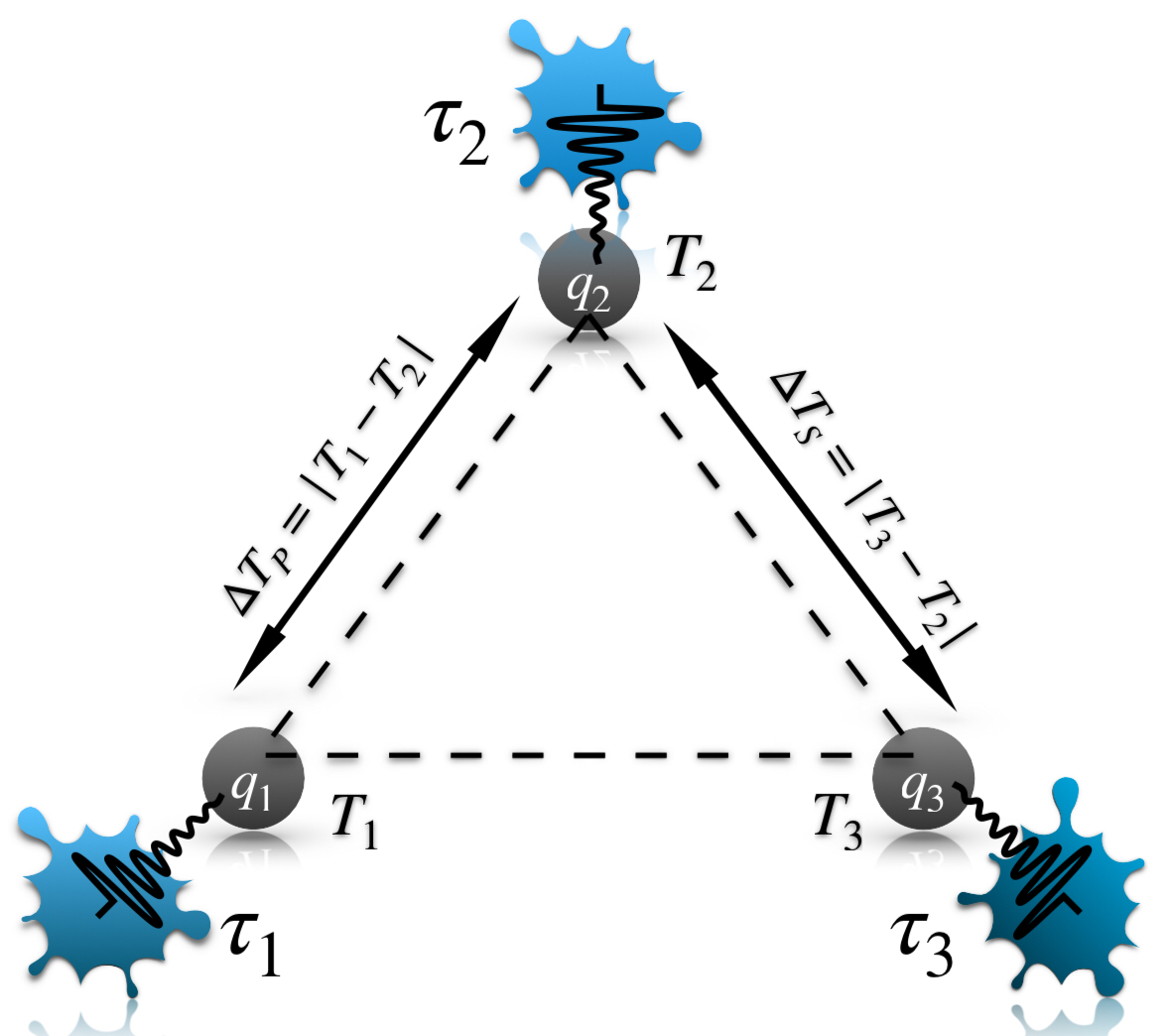
We begin by considering three qubits, labeled as , , and , each locally connected to three thermal reservoirs at temperatures , , and , respectively, and each qubit is in thermal equilibrium with its associated reservoir. Let denote the qubit serving as the common qubit for both the primary and secondary thermal junctions. We take the free Hamiltonian of the three-qubit composite system as , where is the component of the Pauli matrix and is the energy gap between the two levels of the qubit. Here, is a constant with the unit of energy and s are dimensionless energy parameters. Now, the crucial task is to select the interaction Hamiltonian for this three-qubit system that will effectively demonstrate the properties of QHT while ensuring the protocol remains self-contained. To meet the self-contained condition, we find that, for the free system Hamiltonian , various interaction Hamiltonians can be crafted. Without assuming any of the to be zero, the three-qubit free Hamiltonian is subject to some specific self-contained conditions, as follows:
| (1) |
Here, and are the eigenvectors of Pauli- matrix corresponding to the eigenvalues and , respectively. is the dimensionless coupling strength of the interaction. As each qubit resides in its respective thermal state initially, the state of each qubit at the initial time, , can be expressed as
| (2) |
for , , and . Here, is the initial probability to find the qubit in the state . Now, considering the coupling between the systems and their respective reservoirs as weak, we are able to make use of the Born-Markov and secular approximations [29, 30, 31, 32, 33, 34, 35] to govern the evolution of the composite system under the influence of the local thermal baths. Consequently, the dynamics of the reduced system, , can be described using the Gorini-Kossakowski-Sudarshan-Lindblad (GKSL) master equation, as
| (3) |
Here, we introduce the dimensionless time as . We define , and , where can be any of , , , and . The dissipative term, , arises due to the presence of thermal environments. Here runs from to . Additionally, represents the transition frequencies, denotes the decay constants, and are the Lindblad operators. Suppose and represent two eigenvalues of . Then, the transition frequency linked to the transition between these two energy eigenstates is given by . See [29, 30, 31, 32, 33, 35] for detailed discussions on transition energies, decay constants, and the construction of Lindblad operators. For the validation of Born-Markov approximations, the condition, , has to be satisfied. Under the dynamical evolution given by Eq. (3), the reduced density matrices of the individual subsystems, denoted as at any given time , retain their diagonal form as given in Eq. (2). However, in this evolving scenario, the equilibrium probabilities are replaced by time-dependent probabilities and it is connected to the local temperature of each qubit at time as , where is the Boltzmann constant and the index goes to , , and . From now on, we define the dimensionless temperatures of the qubits as and those of the baths as for , , and . Thus, at every instant of time, we have the temperature gradients, for the primary junction, and for the secondary junction. A schematic diagram of this three-qubit QHT is depicted in FIG. 1. To design a step-down quantum transformer, it is essential to ensure that, at any time , .
We now analyze the four self-contained conditions for designing the three-qubit QHTs, given in Eq. (II.1). Let us consider the initial temperature of the three qubits, i.e., the temperature of the three reservoirs follows the condition , and also . In this scenario, one approach to designing an effective QHT involves an increase in the temperature of over time, accompanied by a corresponding decrease in the temperature of . Consequently, the temperature difference at the primary junction at time is expected to increase with time. Conversely, as the temperature of decreases, the temperature of should increase with time. This adjustment ensures that the temperature difference at the secondary junction decreases over time. Therefore, under these circumstances, the condition demands as the interaction Hamiltonian between the qubits, with the choices of parameters facilitating the system transitioning from an initial state of to the state as time progresses with more probability than the opposite process. Note that the interaction Hamiltonian is commonly utilized in the design of quantum refrigerators, as discussed in the literature [8]. However, in this QHT protocol involving the interaction Hamiltonian , does not exhibit the characteristics of a quantum refrigerator. The objective of refrigeration is typically achieved when the qubit with the lowest initial temperature among the three qubits undergoes cooling. Yet, in our protocol, the qubit having the lowest temperature, undergoes a transition to a higher excited state, indicating an increase in its temperature over time. Now, if we alter the considerations and designate as the common qubit, with the initial temperatures of the three reservoirs following the sequence , and , , a parallel methodology reveals as the compatible interaction Hamiltonian. By appropriately selecting parameters with this interaction Hamiltonian, we can ensure that the system initially resides in the state with a higher probability and transitions to the state as time progresses. This transition ensures that over time, the temperature of increases while correspondingly, the temperature of decreases, thereby causing the primary junction temperature difference to increase. Also, the temperature of rises over time to decrease the secondary junction temperature difference . Similarly, if we designate as the common qubit, emerges as the most appropriate Hamiltonian for constructing a QHT for some fixed set of initial conditions.


For a more deeper insight into the operational characteristics of QHTs, we will now delve into the operational aspects of QHTs utilizing the interaction Hamiltonian . Let us consider a scenario where the three qubits are interacting through , and the three thermal baths are bosonic baths, each consisting of an infinite number of harmonic oscillators. Here we set and . The Hamiltonian of each bath can be expressed as
| (4) |
for to . Here the operators () represent the bosonic annihilation (creation) operators corresponding to the energy mode . These operators, having the unit of , satisfy the commutation relation . Here, is an arbitrary constant with units of frequency, and denotes the cutoff frequency for the bath. We take the coupling between the qubit and bath to be
| (5) |
where , a dimensionless function of , modulates the coupling strength of the local interaction between the qubit and bath. Specifically, we have , where denotes the spectral density function of the bosonic bath. For our purposes, we adopt the Ohmic spectral density function, which takes the explicit form . Here s are dimensionless parameters. For the choice of the system-bath intection Hamiltonian given in Eq. (5), we obtain the decay constants as
| (6) | |||||
where being the Bose-Einstein distribution function. Suppose we have two eigenvectors, and , of the system Hamiltonian , corresponding to eigenvalues and respectively. The Lindblad operators for the interaction Hamiltonian [Eq. (5)] can then be written as
| (7) |
Let us now choose the parameters of the system and the interaction Hamiltonians to ensure that the initial probability of finding the qubits in the state exceeds that of . To achieve a higher probability of being in the state initially compared to , the initial composite probability must satisfy the condition
| (8) |
where and . With this initial condition, upon activating the interaction , the transition of the system from the state to the state becomes more probable. In this scenario, qubits and are initially in their ground state, while is in the excited state. With the progress of time, qubits and will transition to their excited state, while will transition to the ground state. Note that the reverse condition of Eq. (8) is also feasible, but we have opted for this particular choice arbitrarily.
In Fig. 2, we illustrate the time evolution of the temperature gradients of the primary () and secondary () thermal junctions, by changing the initial temperature of one of the qubits, say the third qubit . Here we set the initial temperature of as and the initial temperature of as , and vary the value of . For the initial investigation, we set the initial temperature of as . This ensures that at time , we have and . Hence, the difference between the primary and secondary junctions starts at zero. If we now allow the system to evolve under the influence of the thermal baths, we can observe that the difference between and increases over time until it saturates at a value of . See the first panel of Fig. 2. Subsequently, as the initial temperature of decreases incrementally compared to its previous value in different scenarios, as studied in the subsequent panels of Fig. 2, the differences between the saturated values of and reduce, and their differences also decrease. Thus, by adjusting the initial temperature of , we can effectively regulate the performance of the transformer.

Now, the performance of the QHTs can be well understood by defining a parameter, capacity of thermal control (), which quantifies the ability of a QHT to either decrease or increase the temperature of the secondary thermal junction compared to the primary one, for step-down or step-up operation modes respectively. It delineates the degree of temperature alteration achievable in both step-down and step-up operational modes. Let us consider, at any given time , the temperature difference at the primary junction be , and at the secondary junction be . Hence, the capacity of thermal control of a QHT can be defined as
| (9) |
For a step-down quantum transformer, . Conversely, for a step-up QHT, . Based on the analysis of Fig. 2, it is evident that, over a sufficiently long period, the difference varies with alterations in the initial temperature of , represented by . Moreover, we can control by adjusting the initial temperature of or as well. Therefore, can be regulated by the initial temperature of qubits. The relationship between and is depicted in Fig. 3. Here, we have evaluated at time . We observe that monotonically increases with the increase of .


If we examine the interaction Hamiltonian and its self-contained condition, it becomes evident that it yields a negative value, regardless of the chosen values for and . Consequently, for qubit , the state corresponds to the ground state, while the state corresponds to the excited state. When we examine each qubit individually, we observe that the temperatures of and increase over time . However, the temperature of initially decreases for a short period before stabilizing back near to its initial value. So, this QHT scheme is not as straightforward as the previous two cases discussed for and . The most effective approach to comprehend this protocol is by analyzing the rates of temperature change relative to the evolution time, rather than focusing solely on the individual temperature changes of each qubit. The rationale behind constructing the QHT framework using lies in the fact that the rates of temperature change with respect to evolution time differ among the qubits. From Fig. 2, we can infer that the profile of the temperatures is oscillatory, indicating that the quantities will also oscillate around zero, having positive and negative values. Therefore, the rate at which the temperature increases will depend on the absolute values of . Now, to increase the temperature difference between two qubits associated with the primary junction over time through the interaction Hamiltonian , it is crucial for the absolute rate of temperature increase of to be less than the absolute rate of temperature increase of . Consequently, to reduce the temperature difference between two qubits associated with the secondary junction over time, it is necessary for the rate of temperature increase of to be less than the rate of temperature increase of . Additionally, between and , the rate of temperature increase of should be less than the rate of temperature increase of . So, we can write the order of rate of change of temperature of qubits in QHT model involving the interaction Hamiltonian as follows,
| (10) |
For a deeper understanding of these observations, let us consider the scenario depicted in the first panel of Fig. 2. By examining the rate of temperature change for each qubit for this case, as shown in Fig. 4, we find that the absolute values of the rates for , , and , satisfy Eq. (10) in the transient regime. This fulfillment leads to the realization of an effective QHT (see the first panel of Fig. 2). Hence, it is evident that for various sets of initial conditions, we can design three-qubit self-contained QHTs with different interaction Hamiltonians. The operation of these QHTs is contingent upon different conditions related to the local temperature or the change in temperature of the qubits over time. This highlights the strength versatility of the three-qubit QHT model, as it can be tailored to construct a perfectly self-contained QHT model for various initial conditions. We have the flexibility to choose from various configurations for the quantum heat transformer and subsequently select its self-contained interaction Hamiltonian, thus enabling the creation of an intended QHT model.
Now, for completeness, we proceed to discuss another example of a QHT model involving the interaction Hamiltonian , which has already been briefly introduced earlier. In this QHT model, we take the initial temperatures of the three qubits in the order . As previously mentioned, we configure the parameters of the systems and the interaction Hamiltonians such that, , with and . In Fig. 5, we present the operational characteristics of the QHT for this configuration. The temperature gradients of the primary and secondary junctions, and , exhibit a different behavior compared to the case described in Fig. 2. Initially, both and oscillate,and then gradually decrease to reach a steady-state value over time. Furthermore, as the initial temperature of decreases, the steady-state difference between and increases. This indicates that for steady-state regime, increases with the decrease of . This behavior contrasts with the scenario depicted in Fig. 2.
So far, our investigation has focused on cases where the QHT models function as step-down transformers in both steady-state and transient regimes. These models are undeniably crucial for designing effective step-down quantum transformers. However, in certain scenarios, the initial conditions may impose constraints such that they yield a steady-state step-up transformer, whereas the requirement is for a step-down operation. In such cases, a necessarily transient step-down transformer model can prove to be beneficial. The term “necessarily transient step-down transformer” implies that the desired step-down mode can be achieved within the transient domain in an steady-state step-up QHT model. These models hold significance, particularly for specific initial conditions. In the next section, we will present an example of a necessarily transient step-down quantum heat transformer and delve into its operational characteristics.
III Necessarily Transient quantum heat transformers

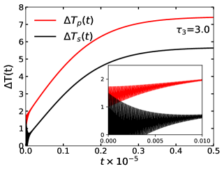
Let us again consider the QHT protocol with the interaction Hamiltonian. As we intend to model a step-up transformer in the steady-state regime, in this model, we need to take the initial temperatures of the three qubits in reverse order compared to the previous step-down configuration. Therefore, it follows: . In this case also, initially we fix the parameters such that . We set the initial temperatures of qubits with equal differences, i.e., at time we set, . The time dynamics of and is shown in Fig. 6 for this situation. We observe that, starting from an equal value, the temperature difference in the primary junction decreases with time. On the other hand, the temperature difference of the secondary junction, increases with time, and the protocol indicates a step-up transformer overall. However, an intriguing discovery emerges upon closer inspection of very small time values. Within this time domain, it becomes apparent that the temperature at the secondary junction falls below that of the primary junction. See the inset of Fig. 6. This observation suggests a step-down configuration, albeit exclusively within a transient domain. We term these QHT models as “the necessarily transient step-down QHT”. This discovery is unique within the QHT protocol, as it reveals that a step-up transformer can exhibit a step-down behavior in the transient domain under specific configurations.
IV Four-qubit QHT
We now move to the four-qubit QHT model consisting of four two level systems, , , , and , locally connected to four thermal baths at temperatures , , , and , respectively. For this model, the primary junction corresponds to qubits and , and the secondary junction corresponds to qubits and . Therefore, there is no shared qubit between the primary and secondary junctions, unlike in the three-qubit QHT model. Here, the temperature gradient at primary junction is given by , and the same for the secondary junction is defined as , with , for , , , and , being the local temperatures of the four qubits, respectively. A schematic diagram of a four-qubit QHT is depicted in Fig. 7.


The free Hamiltonian of the composite four-qubit system is represented by . In a similar manner to the three-qubit system, , various interaction Hamiltonians can also be formulated here, each accompanied by its respective self-contained conditions. Instead of delving into all potential interaction Hamiltonians, we focus on a single example to examine various properties of the four-qubit QHT model. The chosen interaction Hamiltonian and the associated self-contained condition, for this four-qubit model, is given by
| (11) |
Here, is the dimensionless coupling strength. The initial state of the four-qubit system is taken as , for to . We set the parameters s and s for to , such that
| (12) |
This implies that the initial probability of finding the system in the state is higher than that of . Similar to the three-qubit case, we consider the thermal baths as bosonic baths described by the Hamiltonian given in Eq. (4), with system-bath interactions represented by Eq. (5) for to . We now allow the system to evolve under the Markovian dynamics, governed by Eq. (3). The time dynamics of and is demonstrated in Fig. 8. We examine these quantities while varying the initial temperature of . For the case depicted in the first panel of Fig. 8, i.e., for , we observe that the heat difference in the primary junction, , decreases with time. Simultaneously, the heat difference in the secondary junction, , increases with time, ultimately manifesting a step-down behavior. However, in the other two panels, the QHTs exhibit both the nature of a steady-state step-up quantum transformer and the nature of a necessarily transient step-down quantum transformer. For the second case, for , we observe that up to a certain threshold value, the transformer exhibits a step-down behavior, but beyond this threshold, it switches to a step-up mode. With a further increase in from to , the temperature in the secondary junction increases at a faster rate, while the temperature in the primary junction decreases significantly at a faster rate as well. As a result, the step-down mode persists for a very short period of time, and the protocol predominantly functions as a step-up transformer. Therefore, in this four-qubit QHT model, the protocol can be designed to exhibit both step-up and step-down behavior with the same setup, by only varying the initial temperature of , and for fixed initial conditions, we can achieve both step-down and step-up operations in different time regions. This dual nature can also be attained by appropriately adjusting the initial temperature of any one of the qubits. This capability not only expands the versatility of the QHT model but also reduces the design complexity and cost associated with implementing different setups. Note that, in the three-qubit protocols, we can also observe the dual nature discussed in the necessarily transient study. However, the operating region of this necessarily transient phenomenon is very limited, and extending this region is not easily achievable like four-qubit protocol.
V Conclusion
This manuscript aims to establish a protocol for a quantum heat transformer (QHT), resembling the functionality of classical voltage transformers. However, diverging from conventional voltage regulation, a QHT facilitates temperature modulation across its terminals. Our study encompasses the development of self-contained quantum heat transformer models for both three- and four-qubit quantum systems. To explore the operational characteristics of the quantum heat transformer, our focus is specifically on the step-down mode as the primary figure of merit. Initially, we investigate the three-qubit QHT model, serving as the smallest quantum heat transformer configuration. Our findings demonstrate that under various interaction Hamiltonians between the three qubits, the model can function as a self-contained quantum heat transformer. The operation of the QHT protocol relies on the transitions of the qubits between their ground and excited states during the evolution of the system, which impacts the increase or decrease of the local temperatures of the qubits over time. However, in some cases, the behavior of the QHTs cannot be solely explained by changes in local temperatures but also relies on the rate of temperature change of the qubits throughout the evolution of the system. It is important to note that the QHT protocol studied here is analyzed in a generalized manner, allowing for easy switching to the step-up mode as a figure of merit. We define a key performance indicator of a QHT, the capacity of thermal control (), which measures the capability of both step-up and step-down QHTs. Our analysis demonstrates that by precisely adjusting the initial temperatures of the qubits, we can regulate the capacity of thermal control of a QHT. Additionally, we extend our study to four-qubit scenarios, demonstrating the feasibility of constructing self-contained QHTs. An important discovery of our study is the emergence of the necessarily transient step-down QHT model, observed in both the three and four-qubit protocols. In this necessarily transient QHT model, a dual-mode nature is evident, wherein the desired step-down mode can be achieved within the transient domain in an originally step-up QHT model. In the three-qubit protocol, a necessarily transient step-down quantum transformer can be obtained for certain qubit interactions and specific initial conditions within a small transient time regime. Conversely, in the four-qubit protocol, the emergence of necessarily transient step-down quantum transformers is more common. In four-qubit scenarios, we have the advantage of easily tuning the transient regime, enabling the transformer to operate in the intended step-down mode simply by controlling the initial temperatures of the qubits within the same setup. This presents a significant advantage in cost reduction, eliminating the need for distinct setups to achieve step-up and step-down modes. Hence, this novel quantum heat transformer model not only serves as an analog to the classical voltage transformer model but also exhibits advanced characteristics, allowing it to operate as both a step-up and step-down transformer within the same setup, a capability absent in classical voltage transformers.
Acknowledgements.
We acknowledge computations performed using Armadillo [36, 37]. We also acknowledge the use of QIClib – a modern C++ library for general purpose quantum information processing and quantum computing (https://titaschanda.github.io/QIClib) and cluster computing facility at Harish-Chandra Research Institute. AG acknowledges the support from the Alexander von Humboldt Foundation. We acknowledge partial support from the Department of Science and Technology, Government of India through the QuEST grant (grant number DST/ICPS/QUST/Theme-3/2019/120).References
- Alicki and Fannes [2013] R. Alicki and M. Fannes, Entanglement boost for extractable work from ensembles of quantum batteries, Phys. Rev. E 87, 042123 (2013).
- [2] F. Campaioli, F. A. Pollock, and S. Vinjanampathy, Quantum batteries - review chapter, arXiv:1805.05507 [quant-ph] .
- Bhattacharjee and Dutta [2021] S. Bhattacharjee and A. Dutta, Quantum thermal machines and batteries, Eur. Phys. J. B 94, 239 (2021).
- Feldmann and Kosloff [2003] T. Feldmann and R. Kosloff, Quantum four-stroke heat engine: Thermodynamic observables in a model with intrinsic friction, Phys. Rev. E 68, 016101 (2003).
- Kosloff and Levy [2014] R. Kosloff and A. Levy, Quantum heat engines and refrigerators: Continuous devices, Annual Review of Physical Chemistry 65, 365 (2014), pMID: 24689798, https://doi.org/10.1146/annurev-physchem-040513-103724 .
- Mitchison [2019] M. T. Mitchison, Quantum thermal absorption machines: refrigerators, engines and clocks, Contemporary Physics 60, 164 (2019), https://doi.org/10.1080/00107514.2019.1631555 .
- Palao et al. [2001] J. P. Palao, R. Kosloff, and J. M. Gordon, Quantum thermodynamic cooling cycle, Phys. Rev. E 64, 056130 (2001).
- Linden et al. [2010] N. Linden, S. Popescu, and P. Skrzypczyk, How small can thermal machines be? the smallest possible refrigerator, Phys. Rev. Lett. 105, 130401 (2010).
- Levy and Kosloff [2012] A. Levy and R. Kosloff, Quantum absorption refrigerator, Phys. Rev. Lett. 108, 070604 (2012).
- Yuan et al. [2021] Q. Yuan, T. Wang, P. Yu, H. Zhang, H. Zhang, and W. Ji, A review on the electroluminescence properties of quantum-dot-lighting-emitting diodes, Organic Electronics 90, 106086 (2021).
- Chiribella et al. [2013] G. Chiribella, G. M. D’Ariano, P. Perinotti, and B. Valiron, Quantum computations without definite causal structure, Phys. Rev. A 88, 022318 (2013).
- Araújo et al. [2014] M. Araújo, F. Costa, and i. c. v. Brukner, Computational advantage from quantum-controlled ordering of gates, Phys. Rev. Lett. 113, 250402 (2014).
- Ebler et al. [2018] D. Ebler, S. Salek, and G. Chiribella, Enhanced communication with the assistance of indefinite causal order, Phys. Rev. Lett. 120, 120502 (2018).
- Joulain et al. [2016] K. Joulain, J. Drevillon, Y. Ezzahri, and J. Ordonez-Miranda, Quantum thermal transistor, Phys. Rev. Lett. 116, 200601 (2016).
- Zhang et al. [2018] Y. Zhang, Z. Yang, X. Zhang, B. Lin, G. Lin, and J. Chen, Coulomb-coupled quantum-dot thermal transistors, Europhysics Letters 122, 17002 (2018).
- Su et al. [2018] S. Su, Y. Zhang, B. Andresen, and J. Chen, Quantum coherence thermal transistors (2018), arXiv:1811.02400 [quant-ph] .
- Mandarino et al. [2021] A. Mandarino, K. Joulain, M. D. Gómez, and B. Bellomo, Thermal transistor effect in quantum systems, Phys. Rev. Appl. 16, 034026 (2021).
- Aslam et al. [2023] N. Aslam, H. Zhou, E. K. Urbach, M. J. Turner, R. L. Walsworth, M. D. Lukin, and H. Park, Quantum sensors for biomedical applications, Nature Reviews Physics 5, 157 (2023).
- Sarkar et al. [2022] S. Sarkar, C. Mukhopadhyay, A. Alase, and A. Bayat, Free-fermionic topological quantum sensors, Phys. Rev. Lett. 129, 090503 (2022).
- Mishra and Bayat [2021] U. Mishra and A. Bayat, Driving enhanced quantum sensing in partially accessible many-body systems, Phys. Rev. Lett. 127, 080504 (2021).
- Montenegro et al. [2021] V. Montenegro, U. Mishra, and A. Bayat, Global sensing and its impact for quantum many-body probes with criticality, Phys. Rev. Lett. 126, 200501 (2021).
- Martín-Martínez et al. [2013] E. Martín-Martínez, A. Dragan, R. B. Mann, and I. Fuentes, Berry phase quantum thermometer, New Journal of Physics 15, 053036 (2013).
- Sabín et al. [2014] C. Sabín, A. White, L. Hackermuller, and I. Fuentes, Impurities as a quantum thermometer for a bose-einstein condensate, Scientific Reports 4, 6436 (2014).
- Hofer et al. [2017] P. P. Hofer, J. B. Brask, M. Perarnau-Llobet, and N. Brunner, Quantum thermal machine as a thermometer, Phys. Rev. Lett. 119, 090603 (2017).
- Griffiths [1942] D. J. Griffiths, Introduction to electrodynamics (Pearson, Boston, 1942).
- Fitzgerald et al. [2003] A. E. Fitzgerald, C. Kingsley, and S. D. Umans, Electric machinery, 6th ed., McGraw-Hill series in electrical engineering (McGraw-Hill Boston, Mass., Boston, Mass., 2003).
- Purcell and Morin [2013] E. Purcell and D. Morin, Electricity and Magnetism (Cambridge University Press, 2013).
- Skrzypczyk et al. [2011] P. Skrzypczyk, N. Brunner, N. Linden, and S. Popescu, The smallest refrigerators can reach maximal efficiency, Journal of Physics A: Mathematical and Theoretical 44, 492002 (2011).
- Gorini et al. [1976] V. Gorini, A. Kossakowski, and E. C. G. Sudarshan, Completely positive dynamical semigroups of N‐level systems, Journal of Mathematical Physics 17, 821 (1976).
- Lindblad [1976] G. Lindblad, On the generators of quantum dynamical semigroups, Communications in Mathematical Physics 48, 119 (1976).
- Breuer and Petruccione [2002] H. P. Breuer and F. Petruccione, The theory of open quantum systems (Oxford University Press, Great Clarendon Street, 2002).
- Alicki and Lendi [2007] R. Alicki and K. Lendi, Quantum Dynamical Semigroups and Applications (Springer, Berlin, 2007).
- Rivas and Huelga [2011] A. Rivas and S. F. Huelga, Open Quantum Systems, 2191-5423 (Springer Berlin, Heidelberg, 2011).
- Banerjee [2018] S. Banerjee, Open Quantum Systems:Dynamics of Nonclassical Evolution, 2366-8849 (Springer Singapore, 2018).
- [35] D. A. Lidar, Lecture notes on the theory of open quantum systems, arXiv:1902.00967 [quant-ph] .
- Sanderson and Curtin [2016] C. Sanderson and R. Curtin, Armadillo: a template-based C++ library for linear algebra, J. Open Source Softw 1, 26 (2016).
- Sanderson and Curtin [2018] C. Sanderson and R. Curtin, A user-friendly hybrid sparse matrix class in C++, LNCS 10931, 430 (2018).