Quantum geometric tensor and the topological characterization of the extended Su-Schrieffer-Heeger model

The Su-Schrieffer-Heeger (SSH) model is a topological quantum system model with a simple structure, but it has very typical topological properties 1 ; 2 ; 3 ; 4 ; 5 ; 6 , such as the winding number that characterizes the topological properties, the correspondence between bulk states and edge states, etc. 7 ; 8 ; 9 ; 10 ; 11 . In addition, SSH models can be used to describe the one-dimensional polyacetylene, graphene ribbons 12 , p-orbital light ladder systems 13 , and off-diagonal two-color optical lattices 14 . Historically, the Haldane model introduced a next-nearest neighbor inter-action in a two-dimensional honeycomb structure to realize the anomalous quantum Hall effect 9 , causing the system to undergo a topological phase transition from an ordinary insulator to a Chern insulator. Interestingly, if we expand the SSH model by adding appropriate cyclic modulation parameters, we can obtain a phase diagram similar to the two-dimensional Haldane model 15 , which further enriches the theoretical value of the one-dimensional SSH model and can be used to simulate two-dimensional topological systems 16 ; 17 ; 18 ; 19 ; 20 . For the modulated SSH model, all parameters can be obtained by existing cold atom experimental techniques, optical systems or waveguide systems 21 ; 22 ; 23 ; 24 , such as the interaction of fermion atoms on the two-legged ladder 13 , etc., then our results can also be verified by existing experiments.

As a general covariant tensor in Hilbert space geometry, the QGT ${Q_{\mu\nu}}={g_{\mu\nu}}-\frac{i}{2}{F_{\mu\nu}}$ 25 ; 26 defined on a parameterized quantum state manifold is expected to shed some light on understanding quantum phase transitions in many-body systems 27 ; 28 ; 29 . Its imaginary part (up to a coefficient) is right the Berry curvature, which is a key quantity to derive the first Chern number in understand the topological quantum matter. Especially, the quantum metric (real part of the QGT) proposed by Provost and Valee 25 is a positive semi-definite Riemannian metric, which defines a gauge invariant distance between two adjacent quantum states in a parameterized Hilbert space. Recently, it has been shown that the quantum metric plays crucial roles in quantum transport phenomena, quantum noise, optical conductivity, anomalous Hall effect, unconventional superconductivity, and adjacent topics 30 ; 31 ; 32 ; 33 ; 34 ; 35 ; 36 ; 37 ; 38 ; 39 ; 40 ; 41 ; 42 ; 43 ; 44 ; 45 ; 46 ; 47 ; 48 ; 49 ; 50 ; 51 ; 52 ; 53 ; 54 ; 55 ; 56 ; 57 . Furthermore, it has been revealed that the quantum metric can provide a topological Euler number for the energy band, which is based on the Gauss-Bonnet theorem on the topological characterization of the closed Bloch states manifold in the first Brillouin zone. which provides an effective topological index for a class of nontrivial topological phases 58 ; 59 ; 60 ; 61 ; 62 ; 63 ; 64 ; 65 ; 66 ; 67 ; 68 ; 69 ; 70 ; 71 ; 72 .

This paper is structured as follows. In Sec. 2, we study a cyclically modulated SSH model with long-range hop-ping terms, and solve its Hamiltonian in the Bloch momentum space with periodic conditions. In Sec. 3, we obtain the quantum geometric tensor for the occupied lower band of the extended SSH model. The critical points in the model can be witnessed by the singularity behaviors both of the Berry curvature and quantum metric. In Sec. 4, we study the topological Euler number of this model and make a comparison between the phase diagram marked by the Chern number and the Euler number, respectively. Finally, we provide a summary of our work.

We consider the SSH model with N lattice points, the Hamiltonian can be written as 6

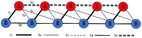
where $\hat{a}_{i}^{\dagger}({\hat{a}_{i}})$ and $\hat{b}_{i}^{\dagger}({\hat{b}_{i}})$ are the creation (annihilation) operators at sublattice A and site B for each $j$-th cell, ${t_{1}}$, ${t_{2}}$ and ${t_{3}}$ represent the nearest-neighbor (NN), next-nearest-neighbor (NNN), and the third-nearest-neighbor (TNN) hopping amplitudes (see Figure 1).

Now, we modulate ${t_{1}}$ and ${t_{2}}$

with ${\theta}$ representing a cyclical parameter varying from 0 to $2\pi$. Meanwhile, ${t_{A}}$ and ${t_{B}}$ are modulated

where $\phi$ is an additional parameter used to adjust the strength relation between ${t_{A}}$ and ${t_{B}}$. Then we consider the periodic boundary conditions and introduce the following Fourier transformation

and the Hamiltonian in momentum space can be written as

where

$h(k,\theta)$ can be written in the form of Pauli matrices

where $\varepsilon\left({k,\theta}\right)$ is the eigenvalue of the Hamiltonian, ${I_{2\times 2}}$ is 2x2 identity matrix, ${d_{\alpha}}(k,\theta)$ is the coefficient of the Pauli matrix, ${\sigma_{\alpha}}$ is a Pauli matrix, representing pseudo-spin degrees of freedom. The diagonalization of $h(k,\theta)$ is straightforward and the eigenvalues can be written as

and the eigenvectors is

Here we choose the following modulated extended SSH model of long-range interactions as an example be-cause it has richer topological properties and higher Chern number topological phases than the ordinary SSH model. In this model, the Hamiltonian of the Bloch state momentum space is

It is obvious that the model is a generalized topological system. When ${t_{3}}={t_{A}}={t_{B}}=0,$ and ${t_{1}}\neq 0$, ${t_{2}}\neq 0$, or when ${t_{1}}({t_{2}})={t_{A}}={t_{B}}=0$ and ${t_{2}}({t_{1}})\neq 0$, the system will degenerate into a one-dimensional SSH model, but when ${t_{3}}=0$ and ${t_{A}}$, ${t_{B}}\neq 0$, the system will become an extended SSH model of next-nearest neighbor interactions. Obviously, for ${t_{A}}={t_{B}}=0$ and ${t_{1}}$, ${t_{2}}$, ${t_{3}}\neq 0$, the model is equal to the two-coupled SSH models.

Firstly, we introduce the quantum geometry tensor in the Bloch momentum space. It is derived from the gauge-invariant metric between two states on the $U(1)$ line bundle. We consider two close wave functions in the parameterized Hilbert space $\left|{\varphi(k)}\right\rangle$ and $\left|{\varphi(k+\delta k)}\right\rangle$, where $k=(\mu,\nu)$ denotes the Hamiltonian parameters $(k,\theta)$ for convenience. The distance between two close wave functions is given by

the extending the factor $\left|{{\partial_{\mu}}\varphi(k){\rm{}}d\mu}\right\rangle$ to

where $P(k)=\left|{\varphi(k)}\right\rangle\left\langle{\varphi(k)}\right|$ is projection operator, $\left|{{D_{\mu}}\varphi(k)}\right\rangle=P(k){\rm{}}\left|{{\partial_{\mu}}\varphi(k)}\right\rangle$ is the covariant derivative of $\left|{\varphi(k)}\right\rangle$. The quantum adiabatic approximation guarantees the parallel transport of the evolution of $\left|{\varphi(k)}\right\rangle$ to $\left|{\varphi(k+\delta k)}\right\rangle$ on the $U(1)$ line bundle, therefore $\left|{{D_{\mu}}\varphi(k)}\right\rangle=0$. We substitute Eq. (11) into Eq. (12) to obtain the quantum metric

And, the quantum geometry tensor is

separating the quantum geometry tensor into the real and the imaginary parts, and we know that the real part is the quantum metric as ${g_{\mu\nu}}={\mathop{\rm Re}\nolimits}{Q_{\mu\nu}}$, and the imaginary part is 1/2 of the negative value of the Berry curvature as ${F_{\mu\nu}}=-2{\mathop{\rm Im}\nolimits}{Q_{\mu\nu}}$, thus we get the quantum geometry tensor for ${Q_{\mu\nu}}={g_{\mu\nu}}-\frac{i}{2}{F_{\mu\nu}}$. And its imaginary part is canceled in the summation of the distance due to its antisymmetric, then the quantum metric can be rewritten as $d{S^{2}}=\sum\nolimits_{\mu\nu}{{\mathop{\rm Re}\nolimits}{Q_{\mu\nu}}d}\mu d\nu$, Given that $P(k)=\left|{\varphi(k)}\right\rangle\left\langle{\varphi(k)}\right|$, substitute it into Eq. (14) to get the quantum geometry tensor:

substituting Eq. (15) into ${F_{\mu\nu}}=-2{\mathop{\rm Im}\nolimits}{Q_{\mu\nu}}$:

then the Berry curvature can be calculated by Eq. (16) and Eq. (9):

where ${\bf{\hat{d}}}$ represents the unit vector ${\bf{d}}/d$ (see 73 for details), and we calculate ${g_{\mu\nu}}={\mathop{\rm Re}\nolimits}{Q_{\mu\nu}}$ according to Eq. (15)

The direct calculations of quantum metric ${g_{\mu\nu}}$ is tedious, however, it can be verified that there is a simple relation between the quantum metric determinant and the Bloch state $\left|{\varphi(k)}\right\rangle$ (for details see the Appendix A in Ref.57 ):

we can get the relationship between quantum metric and Berry curvature by comparing Eq. (17) and Eq. (19):

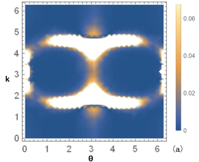
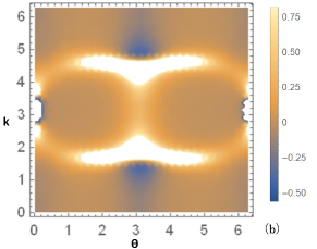
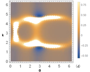
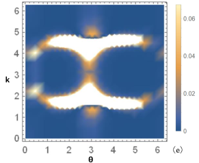
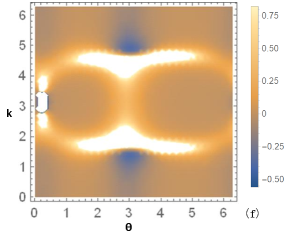
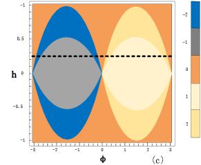
In figure 2, we show the determinant of the quantum metric $\det{g_{\mu\nu}}$ and Berry curvature ${F_{\mu\nu}}$ as the functions of quasi-momentum $\theta,k$ in the first Brillouin zone, with the different modulation parameters.

In the two-dimensional parameters $(\mu,\nu):=(k,\theta)$ space , the topology of the first Brillouin zone is a two-dimensional torus. Considering the Hamiltonian in the two-dimensional momentum space, the Bloch state $\left|{\varphi(k)}\right\rangle$ will adiabatically evolve a $U(1)$ line bundle. The first Chern number, which serves as a topological invariant for all filled bands, can be obtain by integrating the imaginary part (Berry curvature) of the quantum geometry tensor over the Brillouin zone.

Here we assume that the model is half-filled and substitute Eq. (17) into Eq. (21)

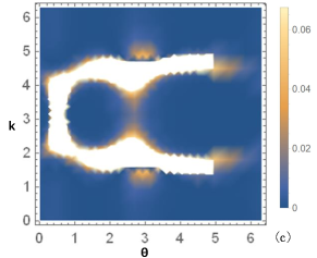
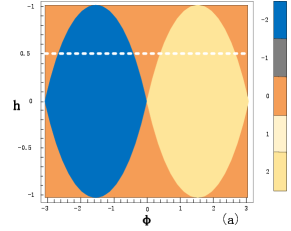
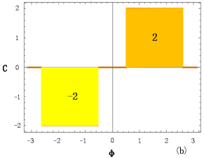
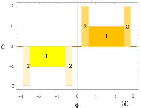
As shown in Figure 3, the model can exhibit different topological phases with higher Chern numbers by varying the next-nearest-neighbor hopping term , and undergoes the corresponding topological quantum phase transitions.

The topological Euler numbers can be derived from the Gauss-Bonnet theorem based on the quantum metric (real part of the quantum geometry tensor)

where $\mathcal{K}={R_{\mu\nu\mu\nu}}/\det g$ is the Gauss curvature, and $dA={(\det g)^{1/2}}d\mu d\nu$ denotes the area measure according to the metric $g$, ${R_{\mu\nu\mu\nu}}$ is the covariant Riemannian curvature tensor. The direct calculation of the Gauss curvature is complicated, but it can be verified that there exists the following relation (for details see the Appendix B in Ref.57 ) in a generalized two-band Hamiltonian on a 2D manifold as ${R_{\mu\nu\mu\nu}}=4\det g$. Then, we generalize Eq. (23) to get the topological Euler number with energy band in the first Brillouin zone.

The numerical results of the topological Euler numbers have been shown in Figure 4 with the Hamiltonian of parameters ${t_{3}}=1$, $h=\frac{1}{2}$.

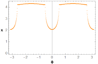
As shown in Figure 4, the Euler number of the lower energy band is not exactly equal to 4 in the topological nontrivial phase where the first Chern number $=\pm 2$. The reason is that the quantum metric tensor is actually positive semi-definite. In a general two-dimensional two-band system, it can be proven that (for more details see Ref.Eulerint ): (1) If the phase is topological trivial, then the quantum metric must be degenerate — det$(g)=0$ in some region of the first Brillouin zone. This leads to the invalidity of the Gauss-Bonnet formula and exhibits an ill-defined “non-integer Euler number”; (2) If the phase is topological nontrivial with a non-vanishing Berry curvature, then the quantum metric will be a positive definite Riemann metric in the entire first Brillouin zone. Therefore the Euler number of the energy band will be guaranteed an even number $2(1-g)$ by the Gauss-Bonnet theorem on the closed two-dimensional Bloch energy band manifold with the genus $g$, which provides an effective topological index for a class of nontrivial topological phases.

In summary, we study the quantum geometry tensor and topological Euler number of an extended SSH model with long-range hopping terms. We show that the phase boundaries of the model can be witnessed by the singularity behaviors both of the Berry curvature and the quantum metric. We also study the topological Euler number of this model and make a comparison between the phase diagram marked by the Chern number and the Euler number, respectively. The degeneracy of the quantum metric in some regions of the first Brillouin zone leads to non-integer Euler numbers. However, the non-integer Euler number can also provide an upper bound for the corresponding Chern numbers Eulerint .

Project supported by the Beijing Natural Science Foundation (Grant No. 1232026), the Qinxin Talents Program of BISTU (Grant No. QXTCP C201711), the R$\&$D Program of Beijing Municipal Education Commission (Grant No. KM202011232017), the National Natural Science Foundation of China (Grant No. 12304190), and the Research fund of BISTU (Grant No. 2022XJJ32).

References

- (1) Su W P, J R Schrieffer, A J Heeger 1979 Phys Rev Let 42 1698
- (2) Hasan M Z and C L Kane 2021 Rev Mod Phys 82 3045
- (3) X L Qi and S C Zhang 2011 Rev Mod Phys 83 1057
- (4) Bansil A, H Lin and T Das 2016 Rev Mod Phys 88 021004
- (5) Witten E 2016 Rev Mod Phys 88 035001
- (6) Li C F, Li X P and Wang L C 2018 EPL 124 37003
- (7) Chiu C K, et al 2016 Rev Mod Phys 88 035005
- (8) Kitaev A Y 2001 Phys Usp 44 131
- (9) Haldane F D M 1988 Phys Rev Let 61 2015
- (10) Qi X L, Wu Y S and Zhang S C 2006 Phys Rev B 74 085308
- (11) Zak J 1989 Phys Rev Let 62 2747
- (12) Delplace P, Ullmo D, and Montambaux. G 2011 Phys Rev B 84 195452
- (13) Li X P, Zhao E H and Vincent L W 2013 Nat Commun 4 195452
- (14) Ganeshan S, Sun K and Das S S 2013 Phys Rev Let 110 180403
- (15) Li L H, Xu Z H and Chen S 2014 Phys Rev B 89 085111
- (16) Takayama H, Lin-Liu Y R and Maki K 1980 Phys Rev B 21 2388
- (17) Su W P, Schrieffer J R and Heeger A J 1980 Phys Rev B 22 2099
- (18) Jackiw R and Rebbi C 1976 Phys Rev D 13 3398
- (19) Heeger A J, et al 1988 Rev Mod Phys 60 781
- (20) Ruostekoski J, Dunne G V and Javanainen J 2002 Phys Rev Let 88 180401
- (21) Li M, Pernice W H P and Tang H X 2009 Nat Photon 3 464
- (22) Weis S, et al 2010 Science 330 1520
- (23) Lin, Q, et al 2009 Phys Rev Let 103 103601
- (24) Xu X, et al 2022 Front Phys 9 813801
- (25) J Provost and G Vallee 1980 Communications in Mathematical Physics 76 289
- (26) Y Q Ma, et al 2010 Phys Rev B 81 245129
- (27) S Sachdev 1999 Quantum Phase Transitions, Cambridge University Press, Cambridge UK
- (28) S L Sondhi, S M Girvin and J P Carini, D Shahar 1997 Rev Mod Phys 69 315
- (29) M Vojta 2003 Rep Prog Phys 66 2069
- (30) T Neupert, L Santos, C Chamon and C Mudry 2011 Phys Rev Let 106 236804
- (31) F Haldane 2004 Phys Rev Let 93 206602
- (32) J W Rhim, K Kim and B J Yang 2020 Nature 584 59
- (33) S Peotta and P T¨orm¨a 2015 Nature Communications 6 8944
- (34) K E Huhtinen, J Herzog-Arbeitman, A Chew, B A Bernevig and P T¨orm¨a 2022 Phys Rev B 106 014518
- (35) Y Gao and D Xiao 2019 Phys Rev Let 122 227402
- (36) M F Lapa and T L Hughes 2019 Phys Rev B 99 121111
- (37) V Kozii, A Avdoshkin, S Zhong and J E Moore 2021 Phys Rev Let 126 156602
- (38) J Mitscherling and T Holder 2022 Phys Rev B 105 085154
- (39) J Ahn, G Y Guo, N Nagaosa and A Vishwanath Nat Phys 18 290
- (40) W Chen and W Huang 2021 Phys Rev Research 3 L042018
- (41) Titus Neupert, et al 2013 Phys Rev B 87 245103
- (42) Srivastava, Ajit, and Ataç Imamoğlu 2015 Phys Rev Let 115 166802
- (43) Victor V Albert, Barry Bradlyn, Martin Fraas and Liang J 2016 Phys Rev X 6 041031
- (44) Tan X S, et al 2019 Phys Rev Let 122 210401
- (45) Ahn Junyeong, Guang-Yu Guo and Naoto Nagaosa 2020 Phys Rev X 10 041041
- (46) Tan X S, et al 2021 Phys Rev Let 126, 017702 (2021).
- (47) Zhi Li, et al 2021 Science China Physics Mechanics and Astronomy 64 107211
- (48) Gonzalesz Diego, Daniel Gutiérrez-Ruiz and J David Vergara 2020 Journal of Physics A: Mathematical and Theoretical 53 505305
- (49) Mera Bruno, Anwei Zhang and Nathan Goldman 2022 SciPost Physics 12 018
- (50) Zhu Y Q, et al 2021 Phys Rev B 104 205103
- (51) Pankaj Bhalla, et al 2021 Phys Rev Let 129 227401
- (52) Li Z, et al 2021 arXiv:2110.11649
- (53) Ding H T, et al 2022 Phys Rev A 105 012210
- (54) Mera Bruno and Johannes Mitscherling 2022 Phys Rev B 106 165133
- (55) Zhai D W, et al 2023 Nature Communications 14 1961
- (56) Y Q Ma and S Chen 2009 Phys Rev A 79 022116
- (57) L Yang, Y Q Ma and X G Li 2015 Physical B 456 359
- (58) Y Q Ma, et al 2013 EPL 103 10008
- (59) Kruchkov Alexander 2022 arXiv:2210.00351
- (60) Kruchkov Alexander 2022 Phys Rev B 105 241102
- (61) Tan X S, et al 2019 Phys Rev Let 122 210401
- (62) Y Q Ma, et al 2013 Phys Let A 377 1250
- (63) Molignini Paolo, et al 2021 Phys Rev B 103 184507
- (64) W Chen and Gero von Gersdorff 2022 arXiv:2202.03494
- (65) G von Gersdorff and W Chen 2019 Phys Rev B 104 195133
- (66) Porlles David and W Chen 2023 arXiv:2306.07366
- (67) Y Q Ma 2014 Phys Rev E 90 042133
- (68) Kolodrubetz Michael, et al 2017 Phys Rep 697 1
- (69) Y Q Ma, et al 2021 EPL 100 60001
- (70) de Sousa, Matheus SM, Antonio L Cruz and Wei Chen 2023 arXiv:2301.06493
- (71) Yi C R, et al 2023 arXiv:2301.06090
- (72) Chen Wei, and Gero von Gersdorff SciPost 2022 Physics Core 5 040
-
(73)
Here we provide the details for the calculation of Berry curvature . For a modulated extended SSH model of long-range interactions in the 2D quasi-momentum space, the Bloch Hamiltonian can be written as , and the unit vector are given by
Then substituting unit vector into Berry curvature , we can obtain
. - (74) Y Q Ma 2020 arXiv:2001.05946