Quantum fluctuation of stress tensor in a higher-derivative scalar field theory around a cosmic string
Abstract
In this paper, we calculate the vacuum fluctuation of the stress tensor of a
higher-derivative theory around a thin cosmic string.
To this end, we adopt the method to obtain the stress tensor from the
effective action developed by Gibbons et al.
By their method, the quantum stress tensor of higher-derivative scalar theories
without self-interaction is expressed as a simple sum of quantum stress tensors of
free massive scalar fields.
Unlike the vacuum expectation value of the
scalar field squared obtained in the similar model, there appears no reduction of
the values near the conical singularity.
Keywords: Higher-derivative theory; quantum fields around a cosmic string.
pacs:
03.70.+k, 04.62.+v, 11.27.+d.I Introduction
The cosmic string Vilenkin ; VS is one of topological defects expected to appear in phase transitions in the very early universe. It has been actively researched as one related to the evolution and structure formation in the early universe. A theoretically interesting thing is that, in the limit of thin strings, the space-time around the cosmic string is locally flat Vilenkin ; VS except for a conical singularity. The behavior of quantum fields in the space-time with such a conical singularity, as a space with nontrivial topology realized in our universe, has been extensively studied until now HK ; Linet ; FS ; Dowker1 ; Dowker2 ; Smith ; AE ; SH ; CKV ; GL ; Moreira ; FP .
The study of quantum fields in the vicinity of singularity may reveal the essential feature of quantum gravity, which is incompletely defined at the present time. In particular, the consequence of theoretical models in nontrivial space-time may give some hints for quantum physics in strong gravity.
Now, there is a nontrivial expectation that the problems of divergence in quantum field theory in the ultraviolet region will be solved by incorporating quantum gravity. Some kind of quantum-gravitational correction is considered to be added to the standard quantum field theory, and a number of models with nonlocality or higher-derivative operators has been studied Modesto ; BT ; AP ; Anselmi ; BLM ; BLMTY .
We consider the model that Frolov and others first proposed FS1 ; FS2 ; Fujikawa , including an infinite number of derivatives in the present paper. They originally considered such a model for the regularization of physical quantities in field theory. Therefore, the divergence behavior related to interacting fields is expected to be improved. In a previous paper KKSW1 , we calculated the vacuum expectation value of a scalar field squared of the higher-derivative theories in a space with a conical singularity, which is equivalent to that around an ideal cosmic string. It was confirmed that its behavior at a short distance from the singularity was milder than that of the canonical scalar model. However, it is generally not clear whether divergence cancels out for the physical quantity that is directly connected to gravity, such as the quantum fluctuation of the stress tensor.
In this paper, we calculate the vacuum expectation value (in other words, quantum fluctuation) of the stress tensor in the same background space-time. We adopt the method to obtain the stress tensor from the effective action developed by Gibbons et al.GPS , and we investigate the characteristics of this physical quantity in the present model.
The organization of the present paper is as follows. In Sec. II, we formulate the method to obtain vacuum expectation values of the stress tensor in the effective theory. In Sec. III, we numerically evaluate the vacuum expectation values of the stress tensor in the higher-derivative scalar field theory in a conical space. The results are summarized in Sec. IV.
II The expression for the quantum fluctuation of the stress tensor in the higher-derivative theory
In the present paper, we consider the following Lagrangian with higher derivatives on a real scalar field :
| (1) |
where denotes the d’Alembertian and is the covariant derivative. Note that this reduces to the canonical massless scalar field Lagrangian if the “cutoff length” becomes zero. The Green’s function in momentum space of this model first appeared in Refs. FS1 ; FS2 ; Fujikawa . The Green’s function in flat configuration space can be written as KKSW1 111Incidentally, we need to consider an Euclidean space for obtaining the vacuum expectation values from the Green’s function.
| (2) |
where denotes the gamma function. It can be confirmed that the limit reduces this expression to the standard massless Green’s function.
The Lagrangian (1) can be written by using the infinite product as
| (3) |
where . Further, in order to apply the treatment according to Ref. GPS , we rewrite this in the form
| (4) |
where , . Note that in the present model.
Gibbons et al.GPS recently constructed the stress tensor of general higher-derivative theories from their effective Lagrangian. The effective Lagrangian with multiple fields reads
| (5) |
where and . We further obtain the relations, , and from the iterative use of the equations of motion. In the present case, the number of fields is infinite.
Then, the stress tensor of the theory is given by GPS
| (6) |
where is the metric tensor of the background space-time. From this expression, we can obtain the vacuum fluctuation of the stress tensor . To estimate the quantum quantities, the fundamental basis is the Green’s function222Because the Green’s function is proportional to , the quantum fluctuation we treated here is dubbed as the one-loop quantum effect.
| (7) |
where denotes a covariant delta function in this symbolic expression. From the Green’s function and the relations to the original field , it turns out to be
| (8) |
where is the canonical Green’s function of a scalar field with mass . Similarly, one finds . Note also that , since .
Consequently, we find a fairly simple expression for the quantum fluctuation of the stress tensor:
| (9) |
where () denotes the covariant derivative with respect to the coordinates ().
In the following section, we evaluate the vacuum expectation value of the stress tensor near a thin cosmic string using the expression obtained above.
III Numerical calculations of the quantum stress tensor around a conical defect
Now, we can express the vacuum expectation value of the stress tensor, or the quantum stress tensor, in the present model as
| (10) |
where
| (11) |
where is the canonical Green’s function of a free scalar field with mass . Note that the value of is still a “bare” quantity (see, for example, Ref. Smith ). When we consider a nontrivial background space-time, we should understand that the physical quantities are the differences of the quantities from those obtained in the trivial, flat and infinite space-times.
We examine the vacuum expectation values of the stress tensor in a conical space. A conical space, or a space with a conical singularity at the coordinate origin, is described by the metric
| (12) |
where is a constant greater than unity. This metric is equivalent to
| (13) |
where the range of is (). This metric adequately describes a locally flat Euclidean space except for the coordinate origin if . A Lorentzian space-time with a deficit angle is often employed as a model space around a mathematically idealized straight cosmic string Vilenkin ; VS . To obtain the quantum quantities in the space-time, we have only to employ the space-time with the Euclidean signature.
The explicit form of the standard Green’s function in a conical space has already been known CKV ; Moreira ; SH ; KKSW1 ; KKSW0 . To emphasize the difference from the flat space without the singularity, it is natural to define . Then, we find KKSW1 ; KKSW0
| (14) | |||||
where , , , and . Using this “renormalized” Green’s function, we define the renormalized vacuum expectation value of the stress tensor as333At the present stage, one can explicitly check , and thus in this expression of the renormalized stress tensor the former assumption of is irrelevant.
| (15) |
In this model, we thus find
| (16) | |||||
where
| (17) |
where is the Jacobi theta function.
Now, we can evaluate the expectation values of the stress tensor in the present higher-derivative theory, very efficiently using these expressions (15) and (16).
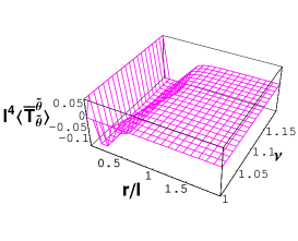
In Fig. 1, we illustrate the dependence of the quantum stress tensor in the present model for . The limit of gives the standard result with a canonical massless scalar field HK ; Linet ; FS ; Dowker1 ; Dowker2 ; Smith ; AE ; SH ; CKV ; GL ; Moreira : and . The correction due to the scale has significant dependence for a fixed . The absolute values of the components of the quantum stress tensor become larger for larger . This behavior is due to the summation form of the stress tensor, in which there is no cancellation as observed in the vacuum expectation value of the scalar squared KKSW1 . Since the contributions from the massive modes exponentially decay at large , asymptotic expressions for the expectation value of the stress tensor are and at large .
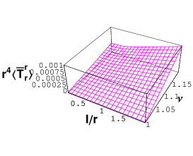
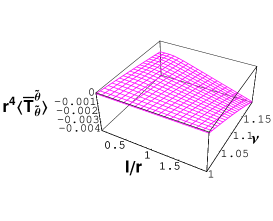
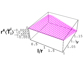
(a) (b) (c)
In Fig. 2, we show the dependence of the quantum stress tensor in the present model. Note that, in Fig. 2, the values near is cut by a certain finite value. The values at are still infinite as in the case with the canonical scalar field HK ; Linet ; FS ; Dowker1 ; Dowker2 ; Smith ; AE ; SH ; CKV ; GL ; Moreira .
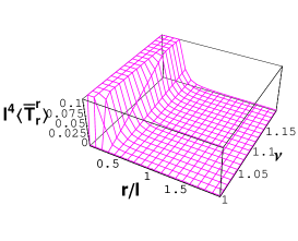
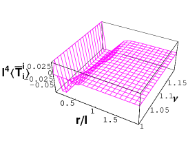
(a) (b) (c)
IV Conclusion
In this paper, we calculated the quantum fluctuations of the stress tensor of a higher-derivative scalar field model FS1 ; FS2 ; Fujikawa in a conical space which looks like a space-time around a cosmic string Vilenkin ; VS . We adopted the stress tensor based on the effective theory of Gibbons et al.GPS . In general, the quantum stress tensor of higher-derivative scalar theories without self-interaction is expressed as a simple sum of quantum stress tensors of free massive scalar fields. Therefore, it was found that there is no cancellation that would appear in the behavior of Green’s function and the vacuum expectation value of a scalar field squared KKSW1 ; some divergences in canonical scalar field theory do not appear in the theory with infinite derivatives. Numerical calculations reveal the dependence of the quantum fluctuation of the stress tensor on the parameter corresponding to the cutoff length included in the theory. It was also confirmed that results coincide with those obtained with the canonical massless scalar field theory Smith in the limit of zero cutoff.
When we introduce self-interaction or interactions of multiple fields, the quantum aspect of higher-derivative theories becomes completely nontrivial. This is because the form of effective interaction becomes inevitably complicated due to the redefinition of the field in effective action. However, if we proceed with utilizing symmetries such as gauge symmetry, we may be able to study physical quantities in certain restricted theories. In addition, it is worthwhile to consider the compact space defined by the boundary condition on fields, where we can perform calculations with considerably ease.
References
- (1) A. Vilenkin, “Cosmic strings and domain walls”, Phys. Rep. 121 (1985) 263.
- (2) A. Vilenkin and E. P. S. Shellard, “Cosmic strings and other topological defects”, (Cambridge Univ. Press, Cambridge, 1994).
- (3) T. M. Helliwell and D. A. Konkowski, “Vacuum fluctuation outside cosmic strings”, Phys. Rev. D34 (1986) 1918.
- (4) B. Linet, “Quantum field theory in the space-time of a cosmic string”, Phys. Rev. D35 (1987) 536.
- (5) V. P. Frolov and E. M. Serebriany, “Vacuum polarization in the gravitational field of a cosmic string”, Phys. Rev. D35 (1987) 3779.
- (6) J. S. Dowker, “Vacuum averages for arbitrary spin around a cosmic string”, Phys. Rev. D36 (1987) 3742.
- (7) J. S. Dowker, in The Formation and Evolution of Cosmic Strings ed G. Gibbons, S. Hawking and T. Vachaspati (Cambridge: Cambridge University Press, 1989) p. 251.
- (8) A. G. Smith, The Formation and Evolution of Cosmic Strings ed G. Gibbons, S. Hawking and T. Vachaspati (Cambridge: Cambridge University Press, 1989) p. 263.
- (9) J. Audretsch and A. Economou, “Quantum-field-theoretical processes near cosmic strings”, Phys. Rev. D44 (1991) 980.
- (10) K. Shiraishi and S. Hirenzaki, “Quantum aspects of self-interacting fields around cosmic strings”, Class. Quant. Grav. 9 (1992) 2277. arXiv:1812.01763 [hep-th].
- (11) G. Cognola, K. Kirsten and L. Vanzo, “Free and self-interacting scalar fields in the presence of conical singularities”, Phys. Rev. D49 (1994) 1029. hep-th/9308106.
- (12) M. E. X. Guimaraes and B. Linet, “Scalar Green’s functions in an Euclidean space with a conical-type line singularity”, Commun. Math. Phys. 165 (1994) 297.
- (13) E. S. Moreira Jnr., “Massive quantum fields in a conical background”, Nucl. Phys. B451 (1995) 365. hep-th/9502016.
- (14) D. Fermi and L. Pizzocchero, Local zeta regularization and the scalar Casimir effect. A general approach based on integral kernels (World Scientific, Singapore, 2017), arXiv:1505.00711, 1505.01044 [math-ph].
- (15) L. Modesto, “Super-renormalizable quantum gravity”, Phys. Rev. D86 (2012) 044005. arXiv:1107.2403 [hep-th].
- (16) T. Biswas and S. Talaganis, “String-inspired infinite-derivative gravity: A brief overview”, Mod. Phys. Lett. A30 (2015) 1540009. arXiv:1412.4256 [gr-qc].
- (17) D. Anselmi and M. Piva, “A new formulation of Lee–Wick quantum field theory”, JHEP 1706 (2017) 066. arXiv:1703.04584 [hep-th].
- (18) D. Anselmi, “The quest for purely virtual quanta: fakeons versus Feynman–Wheeler particles”, JHEP 2003 (2020) 142. arXiv:2001.01942 [hep-th].
- (19) L. Buoninfante, G. Lambiase and A. Mazumdar, “Ghost-free infinite derivative quantum field theory”, Nucl. Phys. B944 (2019) 114646. arXiv:1805.03559 [hep-th].
- (20) L. Buoninfante, G. Lambiase, Y. Miyashita, W. Takebe and M. Yamaguchi, “Generalized ghost-free propagators in nonlocal field theory”, Phys. Rev. D101 (2020) 084019. arXiv:2001.07830 [hep-th].
- (21) S. A. Frolov and A. A. Slavnov, “An invariant regularization of the standard model”, Phys. Lett. B309 (1993) 344.
- (22) S. A. Frolov and A. A. Slavnov, “Removing fermion doublers in chiral gauge theories on the lattice”, Nucl. Phys. B411 (1994) 647. hep-lat/9303004.
- (23) K. Fujikawa, “Generalized Paulli–Villars regularization and the covariant form of anomalies”, Nucl. Phys. B428 (1994) 169. hep-th/9405166.
- (24) N. Kan, M. Kuniyasu, K. Shiraishi and Z.-Y. Wu, “Discrete heat kernel, UV modified Green’s function, and higher derivative theories”, Class. Quant. Grav. 38 (2021) 155002. arXiv:2007.00220 [hep-th].
- (25) G. W. Gibbons, C. N. Pope and S. Solodukhin, “Higher derivative scalar quantum field theory in curved spacetime”, Phys. Rev. D100 (2019) 105008. arXiv:1907.03791 [hep-th].
- (26) N. Kan, M. Kuniyasu, K. Shiraishi and Z.-Y. Wu, “Vacuum expectation values in non-trivial background space from three types of UV improved Green’s functions”, Int. J. Mod. Phys. A36 (2021) 2150001. arXiv:2004.07527 [hep-th].