Quantum electrodynamics in a topological waveguide
Abstract
While designing the energy-momentum relation of photons is key to many linear, non-linear, and quantum optical phenomena, a new set of light-matter properties may be realized by employing the topology of the photonic bath itself. In this work we investigate the properties of superconducting qubits coupled to a metamaterial waveguide based on a photonic analog of the Su-Schrieffer-Heeger model. We explore topologically-induced properties of qubits coupled to such a waveguide, ranging from the formation of directional qubit-photon bound states to topology-dependent cooperative radiation effects. Addition of qubits to this waveguide system also enables direct quantum control over topological edge states that form in finite waveguide systems, useful for instance in constructing a topologically protected quantum communication channel. More broadly, our work demonstrates the opportunity that topological waveguide-QED systems offer in the synthesis and study of many-body states with exotic long-range quantum correlations.
Harnessing the topological properties of photonic bands Haldane and Raghu (2008); Lu et al. (2014); Ozawa et al. (2019) is a burgeoning paradigm in the study of periodic electromagnetic structures. Topological concepts discovered in electronic systems von Klitzing (1986); Hasan and Kane (2010) have now been translated and studied as photonic analogs in various microwave and optical systems Lu et al. (2014); Ozawa et al. (2019). In particular, symmetry-protected topological phases Chen et al. (2013) which do not require time-reversal-symmetry breaking, have received significant attention in experimental studies of photonic topological phenomena, both in the linear and nonlinear regime Smirnova et al. (2019). One of the simplest canonical models is the Su-Schrieffer-Heeger (SSH) model Su et al. (1979); Asbóth et al. (2016), which was initially used to describe electrons hopping along a one-dimensional dimerized chain with a staggered set of hopping amplitudes between nearest-neighbor elements. The chiral symmetry of the SSH model, corresponding to a symmetry of the electron amplitudes found on the two types of sites in the dimer chain, gives rise to two topologically distinct phases of electron propagation. The SSH model, and its various extensions, have been used in photonics to explore a variety of optical phenomena, from robust lasing in arrays of microcavities St-Jean et al. (2017); Zhao et al. (2018) and photonic crystals Ota et al. (2018), to disorder-insensitive 3rd harmonic generation in zigzag nanoparticle arrays Kruk et al. (2019).
Utilization of quantum emitters brings new opportunities in the study of topological physics with strongly interacting photons Carusotto and Ciuti (2013), where single-excitation dynamics Cai et al. (2019) and topological protection of quantum many-body states de Léséleuc et al. (2019) in the SSH model have recently been investigated. In a similar vain, a topological photonic bath can also be used as an effective substrate for endowing special properties to quantum matter. For example, a photonic waveguide which localizes and transports electromagnetic waves over large distances, can form a highly effective quantum light-matter interface Haroche and Raimond (2006); Lodahl et al. (2015); Chang et al. (2018) for introducing non-trivial interactions between quantum emitters. Several systems utilizing highly dispersive electromagnetic waveguide structures have been proposed for realizing quantum photonic matter exhibiting tailorable, long-range interactions between quantum emitters Douglas et al. (2015); Shi et al. (2018); Liu and Houck (2016); Hung et al. (2016). With the addition of non-trivial topology to such a photonic bath, exotic classes of quantum entanglement can be generated through photon-mediated interactions of a chiral Barik et al. (2018); Lodahl et al. (2017) or directional nature Bello et al. (2019); García-Elcano et al. (2019).
With this motivation, here we investigate the properties of quantum emitters coupled to a topological waveguide which is a photonic analog of the SSH model Bello et al. (2019). Our setup is realized by coupling superconducting transmon qubits Koch et al. (2007) to an engineered superconducting metamaterial waveguide Mirhosseini et al. (2018); Ferreira et al. (2020), consisting of an array of sub-wavelength microwave resonators with SSH topology. Combining the notions from waveguide quantum electrodynamics (QED) Lodahl et al. (2015); Chang et al. (2018); Gu et al. (2017); Roy et al. (2017) and topological photonics Lu et al. (2014); Ozawa et al. (2019), we observe qubit-photon bound states with directional photonic envelopes inside a bandgap and cooperative radiative emission from qubits inside a passband dependent on the topological configuration of the waveguide. Coupling of qubits to the waveguide also allows for quantum control over topological edge states, enabling quantum state transfer between distant qubits via a topological channel.
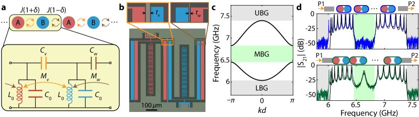
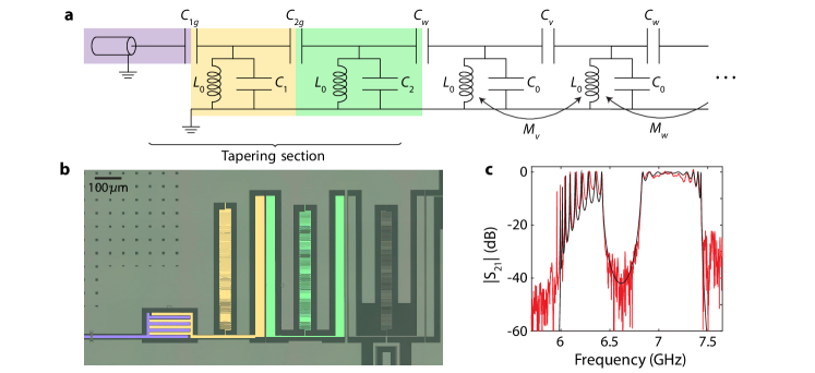
The SSH model describing the topological waveguide studied here is illustrated in Fig. 1a. Each unit cell of the waveguide consists of two photonic sites, A and B, each containing a resonator with resonant frequency . The intra-cell coupling between A and B sites is and the inter-cell coupling between unit cells is . The discrete translational symmetry (lattice constant ) of this system allows us to write the Hamiltonian in terms of momentum-space operators, , where is a vector operator consisting of a pair of A and B sublattice photonic mode operators, and the -dependent kernel of the Hamiltonian is given by,
| (1) |
Here, is the momentum-space coupling between modes on different sublattice, which carries information about the topology of the system. The eigenstates of this Hamiltonian form two symmetric bands centered about the reference frequency with dispersion relation
where the () branch corresponds to the upper (lower) frequency passband. While the band structure is dependent only on the magnitude of , and not on whether or , deformation from one case to the other must be accompanied by the closing of the middle bandgap (MBG), defining two topologically distinct phases. For a finite system, it is well known that edge states localized on the boundary of the waveguide at a only appear in the case of , the so-called topological phase Asbóth et al. (2016); Ozawa et al. (2019). The case for which is the trivial phase with no edge states. It should be noted that for an infinite system, the topological or trivial phase in the SSH model depends on the choice of unit cell, resulting in an ambiguity in defining the bulk properties. Despite this, considering the open boundary of a finite-sized array or a particular section of the bulk, the topological character of the bands can be uniquely defined and can give rise to observable effects.
We construct a circuit analog of this canonical model using an array of inductor-capacitor (LC) resonators with alternating coupling capacitance and mutual inductance as shown in Fig. 1a. The topological phase of the circuit model is determined by the relative size of intra- and inter-cell coupling between neighboring resonators, including both the capacitive and inductive contributions. Strictly speaking, this circuit model breaks chiral symmetry of the original SSH Hamiltonian Asbóth et al. (2016); Ozawa et al. (2019), which ensures the band spectrum to be symmetric with respect to . Nevertheless, the topological protection of the edge states under perturbation in the intra- and inter-cell coupling strengths remains valid under certain conditions, and the existence of edge states still persists due to the presence of inversion symmetry within the unit cell of the circuit analog, leading to a quantized Zak phase Zak (1989). For detailed analysis of the modeling, symmetry, and robustness of the circuit topological waveguide see Apps. A and B.
The circuit model is realized using standard fabrication techniques for superconducting metamaterials discussed in Refs. Mirhosseini et al. (2018); Ferreira et al. (2020), where the coupling between sites is controlled by the physical distance between neighboring resonators. Due to the near-field nature, the coupling strength is larger (smaller) for smaller (larger) distance between resonators on a device. An example unit cell of a fabricated device in the topological phase is shown in Fig. 1b (the values of intra- and inter-cell distances are interchanged in the trivial phase). We find a good agreement between the measured transmission spectrum and a theoretical curve calculated from a LC lumped-element model of the test structures with 8 unit cells in both trivial and topological configurations (Fig. 1c,d). For the topological configuration, the observed peak in the waveguide transmission spectrum at 6.636 GHz inside the MBG signifies the associated edge state physics in our system.
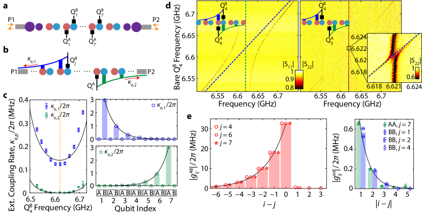
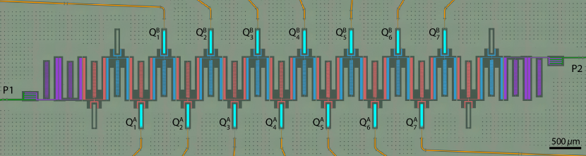
The non-trivial properties of the topological waveguide can be accessed by coupling quantum emitters to the engineered structure. To this end, we prepare Device I consisting of a topological waveguide in the trivial phase with 9 unit cells, whose boundary is tapered with specially designed resonators before connection to external ports (see Fig. 2a). The tapering sections at both ends of the array are designed to reduce the impedance mismatch to the external ports () at frequencies in the upper passband (UPB). This is crucial for reducing ripples in the waveguide transmission spectrum in the passbands Ferreira et al. (2020). The device contains 14 frequency-tunable transmon qubits Koch et al. (2007) coupled to every site on the 7 unit cells in the middle of the array (labeled Q, where 1-7 and =A,B are the cell and sublattice indices, respectively). Properties of Device I and the tapering section are discussed in further detail in Apps. C and D, respectively.
For qubits lying within the middle bandgap, the topology of the waveguide manifests itself in the spatial profile of the resulting qubit-photon bound states. When the qubit transition frequency is inside the bandgap, the emission of a propagating photon from the qubit is forbidden due to the absence of photonic modes at the qubit resonant frequency. In this scenario, a stable bound state excitation forms, consisting of a qubit in its excited state and a waveguide photon with exponentially localized photonic envelope John and Wang (1990); Kurizki (1990). Generally, bound states with a symmetric photonic envelope emerge due to the inversion symmetry of the photonic bath with respect to the qubit location Liu and Houck (2016). In the case of the SSH photonic bath, however, a directional envelope can be realized Bello et al. (2019) for a qubit at the centre of the MBG (), where the presence of a qubit creates a domain wall in the SSH chain and the induced photonic bound state is akin to an edge state (refer to App. E for a detailed description). For example, in the trivial phase, a qubit coupled to site A (B) acts as the last site of a topological array extended to the right (left) while the subsystem consisting of the remaining sites extended to the left (right) is interpreted as a trivial array. Mimicking the topological edge state, the induced photonic envelope of the bound state faces right (left) with photon occupation only on B (A) sites (Fig. 2b), while across the trivial boundary on the left (right) there is no photon occupation. The opposite directional character is expected in the case of the topological phase of the waveguide. The directionality reduces away from the center of the MBG, and is effectively absent inside the upper or lower bandgaps.
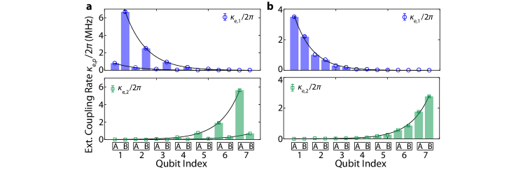
We experimentally probe the directionality of qubit-photon bound states by utilizing the coupling of bound states to the external ports in the finite-length waveguide of Device I (see Fig. 2c). The external coupling rate () is governed by the overlap of modes in the external port with the tail of the exponentially attenuated envelope of the bound state, and therefore serves as a useful measure to characterize the localization Biondi et al. (2014); Liu and Houck (2016); Mirhosseini et al. (2018). To find the reference frequency where the bound state becomes most directional, we measure the external linewidth of the bound state seen from each port as a function of qubit tuning. For Q, which is located near the center of the array, we find to be much larger than at all frequencies inside MBG. At , completely vanishes, indicating a directionality of the Q bound state to the left. Plotting the external coupling at this frequency to both ports against qubit index, we observe a decaying envelope on every other site, signifying the directionality of photonic bound states is correlated with the type of sublattice site a qubit is coupled to. Similar measurements when qubits are tuned to other frequencies near the edge of the MBG, or inside the upper bandgap (UBG), show the loss of directionality away from (App. F).
A remarkable consequence of the distinctive shape of bound states is direction-dependent photon-mediated interactions between qubits (Fig. 2d,e). Due to the site-dependent shapes of qubit-photon bound states, the interaction between qubits becomes substantial only when a qubit on sublattice A is on the left of the other qubit on sublattice B, i.e., for a qubit pair (Q,Q). From the avoided crossing experiments centered at , we extract the qubit-qubit coupling as a function of cell displacement . An exponential fit of the data gives the localization length of (in units of lattice constant), close to the estimated value from the circuit model of our system (see App. C). While theory predicts the coupling between qubits in the remaining combinations to be zero, we report that coupling of and (for ) are observed, much smaller than the bound-state-induced coupling, e.g., . We attribute such spurious couplings to the unintended near-field interaction between qubits. Note that we find consistent coupling strength of qubit pairs dependent only on their relative displacement, not on the actual location in the array, suggesting that physics inside MBG remains intact with the introduced waveguide boundaries. In total, the avoided crossing and external linewidth experiments at provide strong evidence of the shape of qubit-photon bound states, compatible with the theoretical photon occupation illustrated in Fig. 2b.
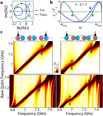
In the passband regime, i.e., when the qubit frequencies lie within the upper or lower passbands, the topology of the waveguide is imprinted on cooperative interaction between qubits and the single-photon scattering response of the system. The topology of the SSH model can be visualized by plotting the complex-valued for values in the first Brillouin zone (Fig. 3a). In the topological (trivial) phase, the contour of encloses (excludes) the origin of the complex plane, resulting in the winding number of 1 (0) and the corresponding Zak phase of (0) Zak (1989). This is consistent with the earlier definition based on the sign of . It is known that for a regular waveguide with linear dispersion, the coherent exchange interaction and correlated decay between qubits at positions and along the waveguide take the forms and Chang et al. (2012); Lalumière et al. (2013), where is the phase length. In the case of our topological waveguide, considering a pair of qubits coupled to A/B sublattice on /-th unit cell, this argument additionally collects the phase Bello et al. (2019). This is an important difference compared to the regular waveguide case, because the zeros of equation
| (2) |
determine wavevectors (and corresponding frequencies) where perfect Dicke super-radiance Dicke (1954) occurs. Due to the properties of introduced above, for a fixed cell-distance between qubits there exists exactly () frequency points inside the passband where perfect super-radiance occurs in the trivial (topological) phase. An example for the case is shown in Fig. 3b. Note that although Eq. (2) is satisfied at the band-edge frequencies and (), they are excluded from the above counting due to breakdown of the Born-Markov approximation that is assumed in obtaining the particular form of cooperative interaction in this picture.
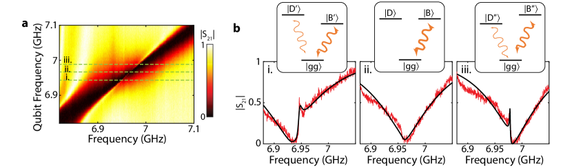
To experimentally probe signatures of perfect super-radiance, we tune the frequency of a pair of qubits across the UPB of Device I while keeping the two qubits resonant with each other. We measure the waveguide transmission spectrum during this tuning, keeping track of the lineshape of the two-qubit resonance as and varies over the tuning. Drastic changes in the waveguide transmission spectrum occur whenever the two-qubit resonance passes through the perfectly super-radiant points, resulting in a swirl pattern in . Such patterns arise from the disappearance of the peak in transmission associated with interference between photons scattered by imperfect super- and sub-radiant states, resembling the electromagnetically-induced transparency in a V-type atomic level structure Witthaut and Sorensen (2010). As an example, we discuss the cases with qubit pairs (Q,Q) and (Q,Q), which are shown in Fig. 3c. Each qubit pair configuration encloses a three-unit-cell section of the waveguide; however for the (Q,Q) pair the waveguide section is in the trivial phase, whereas for (Q,Q) the waveguide section is in the topological phase. Both theory and measurement indicate that the qubit pair (Q,Q) has exactly one perfectly super-radiant frequency point in the UPB. For the other qubit pair (Q,Q), with waveguide section in the topological phase, two such points occur (corresponding to ). This observation highlights the fact that while the topological phase of the bulk in the SSH model is ambiguous, a finite section of the array can still be interpreted to have a definite topological phase. Apart from the unintended ripples near the band-edges, the observed lineshapes are in good qualitative agreement with the theoretical expectation in Ref. Bello et al. (2019). Detailed description of the swirl pattern and similar measurement results for other qubit combinations with varying are reported in App. G.
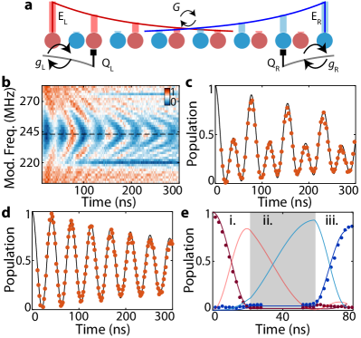
Finally, to explore the physics associated with topological edge modes, we fabricated a second device, Device II, which realizes a closed quantum system with 7 unit cells in the topological phase (Fig. 4a). We denote the photonic sites in the array by (,), where 1-7 is the cell index and A,B is the sublattice index. Due to reflection at the boundary, the passbands on this device appear as sets of discrete resonances. The system supports topological edge modes localized near the sites (1,A) and (7,B) at the boundary, labeled E and E. The edge modes are spatially distributed with exponentially attenuated tails directed toward the bulk. In a finite system, the non-vanishing overlap between the envelopes of edge states generates a coupling which depends on the localization length and the system size as . In Device II, two qubits denoted Q and Q are coupled to the topological waveguide at sites (2,A) and (6,B), respectively. Each qubit has a local drive line and a flux-bias line, which are connected to room-temperature electronics for control. The qubits are dispersively coupled to readout resonators, which are loaded to a coplanar waveguide for time-domain measurement. The edge mode E (E) has photon occupation on sublattice A (B), inducing interaction () with Q (Q). Due to the directional properties discussed earlier, bound states arising from Q and Q have photonic envelopes facing away from each other inside the MBG, and hence have no direct coupling to each other. For additional details on Device II and qubit control, refer to App. H.
We probe the topological edge modes by utilizing the interaction with the qubits. While parking Q at frequency inside MBG, we initialize the qubit into its excited state by applying a microwave -pulse to the local drive line. Then, the frequency of the qubit is parametrically modulated Naik et al. (2017) such that the first-order sideband of the qubit transition frequency is nearly resonant with E. After a variable duration of the frequency modulation pulse, the state of the qubit is read out. From this measurement, we find a chevron-shaped oscillation of the qubit population in time centered at modulation frequency (Fig. 4b). We find the population oscillation at this modulation frequency to contain two harmonic components as shown in Fig. 4c, a general feature of a system consisting of three states with two exchange-type interactions and . In such cases, three single-excitation eigenstates exist at , with respect to the bare resonant frequency of the emitters (), and since the only possible spacing between the eigenstates in this case is and , the dynamics of the qubit population exhibits two frequency components with a ratio of two. From fitting the Q population oscillation data in Fig. 4c, the coupling between E and E is extracted to be . Parking Q at the bare resonant frequency of the edge modes, E strongly hybridizes with Q and is spectrally distributed at with respect to the original frequency (). As this splitting is much larger than the coupling of E to E, the interaction channel EE is effectively suppressed and the vacuum Rabi oscillation only involving Q and E is recovered (Fig. 4d) by applying the above-mentioned pulse sequence on Q. A similar result was achieved by applying a simultaneous modulation pulse on Q to put its first-order sideband near-resonance with the bare edge modes (instead of parking it near resonance), which we call the double-modulation scheme. From the vacuum Rabi oscillation QE (QE) using the double-modulation scheme, we find the effective qubit-edge mode coupling to be ().
The half-period of vacuum Rabi oscillation corresponds to an iSWAP gate between Q and E (or Q and E), which enables control over the edge modes with single-photon precision. As a demonstration of this tool, we perform remote population transfer between Q and Qthrough the non-local coupling of topological edge modes E and E. The qubit Q (Q) is parked at frequency 6.829 GHz (6.835 GHz) and prepared in its excited (ground) state. The transfer protocol, consisting of three steps, is implemented as follows: i) an iSWAP gate between Q and E is applied by utilizing the vacuum Rabi oscillation during the double-modulation scheme mentioned above, ii) the frequency modulation is turned off and population is exchanged from E to E using the interaction , iii) another iSWAP gate between Q and E is applied to map the population from E to Q. The population of both qubits at any time within the transfer process is measured using multiplexed readout Chen et al. (2012) (Fig. 4e). We find the final population in Q after the transfer process to be 87 %. Numerical simulations suggest that (App. H) the infidelity in preparing the initial excited state accounts for 1.6 % of the population decrease, the leakage to the unintended edge mode due to ever-present interaction contributes 4.9 %, and the remaining 6.5 % is ascribed to the short coherence time of qubits away from the flux-insensitive point [ ns for Q (Q) at working point].
We expect that a moderate improvement on the demonstrated population transfer protocol could be achieved by careful enhancement of the excited state preparation and the iSWAP gates, i.e. optimizing the shapes of the control pulses Khaneja et al. (2005); Motzoi et al. (2009); Didier et al. (2018); Hong et al. (2020). The coherence-limited infidelity can be mitigated by utilizing a less flux-sensitive qubit design Sete et al. (2017); Hutchings et al. (2017) or by reducing the generic noise level of the experimental setup Ott (2009). Further, incorporating tunable couplers Chen et al. (2014) into the existing metamaterial architecture to control the localization length of edge states in situ will fully address the population leakage into unintended interaction channels, and more importantly, enable robust quantum state transfer over long distances Lang and Büchler (2017). Together with many-body protection to enhance the robustness of topological states de Léséleuc et al. (2019), building blocks of quantum communication Kimble (2008) under topological protection are also conceivable.
Looking forward, we envision several research directions to be explored beyond the work presented here. First, the topology-dependent photon scattering in photonic bands that is imprinted in the cooperative interaction of qubits can lead to new ways of measuring topological invariants in photonic systems Tran et al. (2017). The directional and long-range photon-mediated interactions between qubits demonstrated in our work also opens avenues to synthesize non-trivial quantum many-body states of qubits, such as the double Néel state Bello et al. (2019). Even without technical advances in fabrication Dunsworth et al. (2018); Rosenberg et al. (2017); Foxen et al. (2017), a natural scale-up of the current system will allow for the construction of moderate to large-scale quantum many-body systems. Specifically, due to the on-chip wiring efficiency of a linear waveguide QED architecture, with realistic refinements involving placement of local control lines on qubits and compact readout resonators coupled to the tapered passband (intrinsically acting as Purcell filters Jeffrey et al. (2014)), we expect that a fully controlled quantum many-body system consisting of 100 qubits is realizable in the near future. In such systems, protocols for preparing and stabilizing de Léséleuc et al. (2019); Ma et al. (2017, 2019) quantum many-body states could be utilized and tested. Additionally, the flexibility of superconducting metamaterial architectures Mirhosseini et al. (2018); Ferreira et al. (2020) can be further exploited to realize other novel types of topological photonic baths Lodahl et al. (2017); Bello et al. (2019); García-Elcano et al. (2019). While the present work was limited to a one-dimensional system, the state-of-the-art technologies in superconducting quantum circuits Krantz et al. (2019) utilizing flip-chip methods Rosenberg et al. (2017); Foxen et al. (2017) will enable integration of qubits into two-dimensional metamaterial surfaces. It also remains to be explored whether topological models with broken time-reversal symmetry, an actively pursued approach in systems consisting of arrays of three-dimensional microwave cavities Anderson et al. (2016); Owens et al. (2018), could be realized in compact chip-based architectures. Altogether, our work sheds light on opportunities in superconducting circuits to explore quantum many-body physics originating from novel types of photon-mediated interactions in topological waveguide QED, and paves the way for creating synthetic quantum matter and performing quantum simulation Blatt and Roos (2012); Gross and Bloch (2017); Lewis-Swan et al. (2019); Georgescu et al. (2014); Carusotto et al. (2020).
Acknowledgements.
The authors thank Xie Chen and Hans Peter Büchler for helpful discussions. We also appreciate MIT Lincoln Laboratories for the provision of a traveling-wave parametric amplifier used for both spectroscopic and time-domain measurements in this work, and Jen-Hao Yeh and B. S. Palmer for the cryogenic attenuators for reducing thermal noise in the metamaterial waveguide. This work was supported by the AFOSR MURI Quantum Photonic Matter (grant FA9550-16-1-0323), the DOE-BES Quantum Information Science Program (grant DE-SC0020152), the AWS Center for Quantum Computing, the Institute for Quantum Information and Matter, an NSF Physics Frontiers Center (grant PHY-1125565) with support of the Gordon and Betty Moore Foundation, and the Kavli Nanoscience Institute at Caltech. V.F. gratefully acknowledges support from NSF GFRP Fellowship. A.S. is supported by IQIM Postdoctoral Fellowship. A.G.-T. acknowledges funding from project PGC2018-094792-B-I00 (MCIU/AEI/FEDER, UE), CSIC Research Platform PTI-001, and CAM/FEDER Project No. S2018/TCS-4342 (QUITEMAD-CM).Appendix A Modeling of the topological waveguide
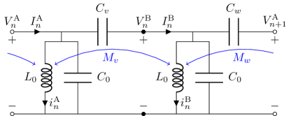
In this section we provide a theoretical description of the topological waveguide discussed in the main text, an analog to the Su-Schrieffer-Heeger model Su et al. (1979). An approximate form of the physically realized waveguide is given by an array of coupled LC resonators, a unit cell of which is illustrated in Fig. 5. Each unit cell of the topological waveguide has two sites A and B whose intra- and inter-cell coupling capacitance (mutual inductance) are given by () and (). We denote the flux variable of each node as and the current going through each inductor as (). The Lagrangian in position space reads
| (3) |
The node flux variables are written in terms of current through the inductors as
| (4) |
Considering the discrete translational symmetry in our system, we can rewrite the variables in terms of Fourier components as
| (5) |
where , is the number of unit cells, and () are points in the first Brillouin zone. Equation (4) is written as
under this transform. Multiplying the above equation with and summing over all , we get a linear relation between and :
By calculating the inverse of this relation, the Lagrangian of the system (3) can be rewritten in -space as
| (6) |
where and . The node charge variables canonically conjugate to node flux are
Note that due to the Fourier transform implemented on flux variables, the canonical charge in momentum space is related to that in real space by
which is in the opposite sense of regular Fourier transform in Eq. (5). Also, due to the Fourier-transform properties, the constraint that and are real reduces to and . Applying the Legendre transformation , the Hamiltonian takes the form
where
Note that and are real and even function in . We impose the canonical commutation relation between real-space conjugate variables to promote the flux and charge variables to quantum operators. This reduces to in the momentum space [Note that due to the Fourier transform, and , meaning flux and charge operators in momentum space are non-Hermitian since the Hermitian conjugate flips the sign of ]. The Hamiltonian can be written as a sum , where the “uncoupled” part and coupling terms are written as
| (7) |
with the effective self-capacitance , self-inductance , coupling capacitance , and coupling inductance given by
| (8) |
The diagonal part of the Hamiltonian can be written in a second-quantized form by introducing annihilation operators and , which are operators of the Bloch waves on A and B sublattice, respectively:
Here, is the effective impedance of the oscillator at wavevector . Unlike the Fourier transform notation, for bosonic modes and , we use the notation and . Under this definition, the commutation relation is rewritten as . Note that the flux and charge operators are written in terms of mode operators as
The uncoupled Hamiltonian is written as
| (9) |
where the “uncoupled” oscillator frequency is given by , which ranges between values
The coupling Hamiltonian is rewritten as
| (10) |
where the capacitive coupling and inductive coupling are simply written as
| (11) |
respectively. Note that and . In the following, we discuss the diagonalization of this Hamiltonian to explain the dispersion relation and band topology.
A.1 Band structure within the rotating-wave approximation
We first consider the band structure of the system within the rotating-wave approximation (RWA), where we discard the counter-rotating terms and in the Hamiltonian. This assumption is known to be valid when the strength of the couplings , are small compared to the uncoupled oscillator frequency . Under this approximation, the Hamiltonian in Eqs. (9)-(10) reduces to a simple form , where the single-particle kernel of the Hamiltonian is,
| (12) |
Here, is the vector of annihilation operators at wavevector and . In this case, the Hamiltonian is diagonalized to the form
| (13) |
where two bands symmetric with respect to at each wavevector appear [here, note that ]. The supermodes are written as
where is the phase of coupling term. The Bloch states in the single-excitation bands are written as
where denotes a state with () photons in mode ().
As discussed below in App. B, the kernel of the Hamiltonian in Eq. (12) has an inversion symmetry in the sublattice unit cell which is known to result in bands with quantized Zak phase Zak (1989). In our system the Zak phase of the two bands are evaluated as
The Zak phase of photonic bands is determined by the behavior of in the complex plane. If the contour of for values in the first Brillouin zone excludes (encloses) the origin, the Zak phase is given by () corresponding to the trivial (topological) phase.
A.2 Band structure beyond the rotating-wave approximation
Considering all the terms in the Hamiltonian in Eqs. (9)-(10), the Hamiltonian can be written in a compact form with a vector composed of mode operators and
| (14) |
where as before and . Here, and are inductive and capacitive coupling normalized to frequency. The dispersion relation can be found by diagonalizing the kernel of the Hamiltonian in Eq. (14) with the Bogoliubov transformation
| (15) |
where is the vector composed of supermode operators and , are matrices forming blocks in the transformation . We want to find such that , where is diagonal. To preserve the commutation relations, the matrix has to be symplectic, satisfying , with defined as
Due to this symplecticity, it can be shown that the matrices and are similar under transformation . Thus, finding the eigenvalues and eigenvectors of the coefficient matrix
| (16) |
is sufficient to obtain the dispersion relation and supermodes of the system. The eigenvalues of matrix are evaluated as
and hence the dispersion relation of the system taking into account all terms in Hamiltonian (14) is
| (17) |
where
The two passbands range over frequencies and , where the band-edge frequencies are written as
| (18a) | |||
| (18b) |
Here, and are sign factors. In principle, the eigenvectors of the matrix in Eq. (16) can be analytically calculated to find the transformation of the original modes to supermodes . For the sake of brevity, we perform the calculation in the limit of vanishing mutual inductance (), where the matrix reduces to
| (19) |
In this case, the block matrices , in the transformation in Eq. (15) are written as
where , , and . Note that the constants are normalized by relation .
The knowledge of the transformation allows us to evaluate the Zak phase of photonic bands. In the Bogoliubov transformation, the Zak phase can be evaluated as Goren et al. (2018)
identical to the expression within the RWA. Again, the Zak phase of photonic bands is determined by the winding of around the origin in complex plane, leading to in the trivial phase and in the topological phase.
A.3 Extraction of circuit parameters and the breakdown of the circuit model
As discussed in Fig. 1d of the main text, the parameters in the circuit model of the topological waveguide is found by fitting the waveguide transmission spectrum of the test structures. We find that two lowest-frequency modes inside the lower passband fail to be captured according to our model with capacitively and inductively coupled LC resonators. We believe that this is due to the broad range of frequencies (about 1.5 GHz) covered in the spectrum compared to the bare resonator frequency and the distributed nature of the coupling, which can cause our simple model based on frequency-independent lumped elements (inductor, capacitor, and mutual inductance) to break down. Such deviation is also observed in the fitting of waveguide transmission data of Device I (Fig. 11).
Appendix B Mapping of the system to the SSH model and discussion on robustness of edge modes
B.1 Mapping of the topological waveguide to the SSH model
We discuss how the physical model of topological waveguide in App. A could be mapped to the photonic SSH model, whose Hamiltonian is given as Eq. (1) in the main text. Throughout this section, we consider the realistic circuit parameters extracted from fitting of test structures given in Fig. 1 of the main text: resonator inductance and resonator capacitance, and , and coupling capacitance and parasitic mutual inductance, and in the trivial phase (the values are interchanged in the topological phase).
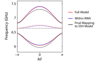
To most directly and simply link the Hamiltonian described in Eqs. (9)-(10) to the SSH model, here we impose a few approximations. First, the counter-rotating terms in the Hamiltonian are discarded such that only photon-number-conserving terms are left. To achieve this, the RWA is applied to reduce the kernel of the Hamiltonian into one involving a matrix as in Eq. (12). Such an assumption is known to be valid when the coupling terms in the Hamiltonian are much smaller than the frequency scale of the uncoupled Hamiltonian Kockum et al. (2019). According to the coupling terms derived in Eq. (11), this is a valid approximation given that
and the RWA affects the dispersion relation by less than 0.3 % in frequency.
Also different than in the original SSH Hamiltonian, are the -dependent diagonal elements of the single-particle kernel of the Hamiltonian for the circuit model. This -dependence can be understood as arising from the coupling between resonators beyond nearest-neighbor pairs, which is inherent in the canonical quantization of capacitively coupled LC resonator array (due to circuit topology) as discussed in Ref. Ferreira et al. (2020). The variation in can be effectively suppressed in the limit of and as derived in Eq. (8). We note that while our coupling capacitances are small compared to (, in the trivial phase), we find that they are sufficient to cause the to vary by 1.2 % in the first Brillouin zone. Considering this limit of small coupling capacitance and mutual inductance, the effective capacitance and inductance of (8) become quantities independent of , , , and the kernel of the Hamiltonian under RWA reduces to
Here,
This is equivalent to the photonic SSH Hamiltonian in Eq. (1) of the main text under redefinition of gauge which transforms operators as . Here, we can identify the parameters and as
| (20) |
where is defined as intra-cell and inter-cell coupling, respectively. The dispersion relations under different stages of approximations mentioned above are plotted in Fig. 6, where we find a clear deviation of our system from the original SSH model due to the -dependent reference frequency.
B.2 Robustness of edge modes under perturbation in circuit parameters
While we have linked our system to the SSH Hamiltonian in Eq. (1) of the main text, we find that our system fails to strictly satisfy chiral symmetry ( is the chiral symmetry operator in the sublattice space). This is due to the -dependent diagonal terms in , resulting from the non-local nature of the quantized charge and nodal flux in the circuit model which results in next-nearest-neighbor coupling terms between sublattices of the same type. Despite this, an inversion symmetry, ( in the sublattice space), still holds for the circuit model. This ensures the quantization of the Zak phase () and the existence of an invariant band winding number () for perturbations that maintain the inversion symmetry. However, as shown in Refs. Pérez-González et al. (2018); Longhi (2018), the inversion symmetry does not protect the edge states for highly delocalized coupling along the dimer resonator chain, and the correspondence between winding number and the number of localized edge states at the boundary of a finite section of waveguide is not guaranteed.
For weak breaking of the chiral symmetry (i.e., beyond nearest-neighbor coupling much smaller than nearest neighbor coupling) the correspondence between winding number and the number of pairs of gapped edge states is preserved, with winding number in the trivial phase () and in the topological () phase. Beyond just the existence of the edge states and their locality at the boundaries, chiral symmetry is special in that it pins the edge mode frequencies at the center of the middle bandgap (). Chiral symmetry is maintained in the presence of disorder in the coupling between the different sublattice types along the chain, providing stability to the frequency of the edge modes. In order to study the robustness of the edge mode frequencies in our circuit model, we perform a simulation over different types of disorder realizations in the circuit illustrated in Fig. 5. As the original SSH Hamiltonian with chiral symmetry gives rise to topological edge states which are robust against the disorder in coupling, not in on-site energies Asbóth et al. (2016), it is natural to consider disorder in circuit elements that induce coupling between resonators: , , , .
The classical equations of motion of a circuit consisting of unit cells is written as
where the superscripts indicate index of cell of each circuit element and
The coupled differential equations are rewritten in a compact form as
| (21) |
where the coefficient matrix is given by
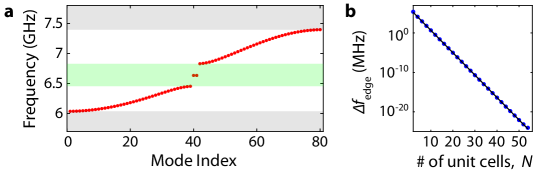
Here, the matrix elements not specified are all zero. The resonant frequencies of the system can be determined by finding the positive eigenvalues of . Considering the model without any disorder, we find the eigenfrequencies of the finite system to be distributed according to the passband and bandgap frequencies from dispersion relation in Eq. (17), as illustrated in Fig. 7. Also, we observe the presence of a pair of coupled edge mode resonances inside the middle bandgap in the topological phase, whose splitting due to finite system size scales as with .
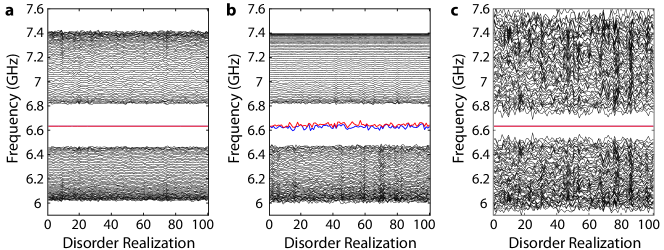
To discuss the topological protection of the edge modes, we keep track of the set of eigenfrequencies for different disorder realizations of the coupling capacitance and mutual inductance for a system with unit cells. First, we consider the case when the mutual inductance and between resonators are subject to disorder. The values of , are assumed to be sampled uniformly on an interval covering a fraction of the original values, i.e.,
where are independent random numbers uniformly sampled from an interval . Figure 8a illustrates an example with a strong disorder with under 100 independent realizations, where we find the frequencies of the edge modes to be stable, while frequencies of modes in the passbands fluctuate to a much larger extent. This suggests that the frequencies of edge modes have some sort of added robustness against disorder in the mutual inductance between neighboring resonators despite the fact that our circuit model does not satisfy chiral symmetry. The reduction in sensitivity results from the fact that the effective self-inductance of the resonators, which influences the on-site resonator frequency, depends on the mutual inductances only to second-order in small parameter . It is this second-order fluctuation in the resonator frequencies, causing shifts in the diagonal elements of the Hamiltonian, which results in fluctuations in the edge mode frequencies. The direct fluctuation in the mutual inductance couplings themselves, corresponding to off-diagonal Hamiltonian elements, do not cause the edge modes to fluctuate due to chiral symmetry protection (the off-diagonal part of the kernel of the Hamiltonian is chiral symmetric).
Disorder in coupling capacitance and are also investigated using a similar model, where the values of , are allowed to vary by a fraction of the original values (uniformly sampled), while the remaining circuit parameters are kept constant. From Fig. 8b we observe severe fluctuations in the frequencies of the edge modes even under a mild disorder level of . This is due to the fact that the coupling capacitance and contribute to the effective self-capacitance of each resonator to first-order in small parameter , thus directly breaking chiral symmetry and causing the edge modes to fluctuate. An interesting observation in Fig. 8b is the stability of frequencies of modes in the upper passband with respect to disorder in and . This can be explained by noting the expressions for band-edge frequencies in Eqs. (18a)-(18b), where the dependence on coupling capacitance gets weaker close to the upper band-edge frequency of the upper passband.
Finally, we consider a special type of disorder where we keep the bare self-capacitance of each resonator fixed. Although unrealistic, we allow and to fluctuate and compensate for the disorder in by subtracting the deviation in and from . This suppresses the lowest-order resonator frequency fluctuations, and hence helps stabilize the edge mode frequencies even under strong disorder , as illustrated in Fig. 8c. While being an unrealistic model for disorder in our physical system, this observation sheds light on the fact that the circuit must be carefully designed to take advantage of the topological protection. It should also be noted that in all of the above examples, the standard deviation in the edge mode frequencies scale linearly to lowest order with the standard deviation of the disorder in the inter- and intra-cell coupling circuit elements (only the pre-coefficient changes). Exponential suppression of edge mode fluctuations due to disorder in the coupling elements as afforded by the SSH model with chiral symmetry would require a redesign of the circuit to eliminate the next-nearest-neighbor coupling present in the current circuit layout.
Appendix C Device I characterization and Experimental setup
In this section, we provide a detailed description of elements on Device I, where the directional qubit-photon bound state and passband topology experiments are performed. The optical micrograph of Device I is shown in Fig. 9.
[t] Q Q Q Q Q Q Q Q Q Q Q Q Q Q (kHz) 325.7 150.4 247.4 104.7a 268.2 183.2 220.6 224.4 193.3 263.2 206 332.69 88.1 346.8
-
a
Measured in a separate cooldown
C.1 Qubits
All 14 qubits on Device I are designed to be nominally identical with asymmetric Josephson junctions (JJs) on superconducting quantum interference device (SQUID) loop to reduce the sensitivity to flux noise away from maximum and minimum frequencies, referred to as “sweet spots”. The sweet spots of all qubits lie deep inside the upper and lower bandgaps, where the coupling of qubits to external ports are small due to strong localization. This makes it challenging to access the qubits with direct spectroscopic methods near the sweet spots. Alternatively, a strong drive tone near resonance with a given qubit frequency was sent into the waveguide to excite the qubit, and a passband mode dispersively coupled to the qubit is simultaneously monitored with a second probe tone. With this method, the lower (upper) sweet spot of Q is found to be at 5.22 GHz (8.38 GHz), and the anharmonicity near the upper sweet spot is measured to be 297 MHz (effective qubit capacitance of ). The Josephson energies of two JJs of Q are extracted to be giving the junction asymmetry of .
The coherence of qubits is characterized using spectroscopy inside the middle bandgap (MBG). Here, the parasitic decoherence rate is defined as , where is the total linewidth of qubit, and () is the external coupling rate to port 1 (2) (see Supplementary Note 1 of Ref. Mirhosseini et al. (2019) for a detailed discussion). Here, contains contributions from both qubit decay to spurious channels other than the desired external waveguide as well as pure dephasing. Table 1 shows the parasitic decoherence rate of all 14 qubits at 6.621 GHz extracted from spectroscopic measurement at a power at least 5 dB below the single-photon level (defined as with ) from both ports.
Utilizing the dispersive coupling between the qubit and a resonator mode in the passband, we have also performed time-domain characterization of qubits. The measurement on Q at 6.605 GHz in the MBG gives and corresponding to , consistent with the result from spectroscopy in Table 1. At the upper sweet spot, Q was hard to access due to the small coupling to external ports arising from short localization length and a large physical distance from the external ports. Instead, Q is characterized to be and at its upper sweet spot (8.569 GHz).
C.2 Metamaterial waveguide and coupling to qubits
As shown in Fig. 9, the metamaterial waveguide consists of a SSH array in the trivial configuration and tapering sections at the boundary (the design of tapering sections is discussed in App. D). The array contains 18 identical LC resonators, whose design is slightly different from the one in test structures shown in Fig. 1b of the main text. Namely, the “claw” used to couple qubits to resonators on each site is extended to generate a larger coupling capacitance of and the resonator capacitance to ground was reduced accordingly to maintain the designed reference frequency. On resonator sites where no qubit is present, an island with shape identical to that of a qubit was patterned and shorted to ground plane in order to mimic the self-capacitance contribution from a qubit to the resonator. The fitting of the whole structure to the waveguide transmission spectrum results in a set of circuit parameters similar yet slightly different from ones of the test structures quoted in Fig. 1 of the main text: , , , . Here, the definition of includes contributions from coupling capacitance between qubit and resonator, but excludes the contribution to the resonator self-capacitance from the coupling capacitances , between resonators in the array. With these parameters we calculate the corresponding parameters in the SSH model to be and following Eq. (20), resulting in the localization length at the reference frequency. From the measured avoided crossing between qubit-photon bound states facing toward each other on nearest-neighboring sites together with and , we infer the qubit coupling to each resonator site to be Bello et al. (2019), close to the value
expected from designed coupling capacitance Sank (2014). Note that we find an inconsistent set of values and (with and accordingly) from calculation based on the difference in observed band-edge frequencies, where the frequency difference between the highest frequency in the UPB and the lowest frequency in the LPB equals and the size of the MBG equals . The inconsistency indicates the deviation of our system from the proposed circuit model (see App. A for discussion), which accounts for the difference between theoretical curves and the experimental data in Fig. 1d and left sub-panel of Fig. 2c. The values of and from the band-edge frequencies are used to generate the theoretical curves in Fig. 3 in the main text as well as in Fig. 15. The intrinsic quality factor of one of the normal modes (resonant frequency 6.158 GHz) of the metamaterial waveguide was measured to be at power below the single-photon level, similar to typical values reported in Refs. Mirhosseini et al. (2018); Ferreira et al. (2020).
C.3 Experimental setup
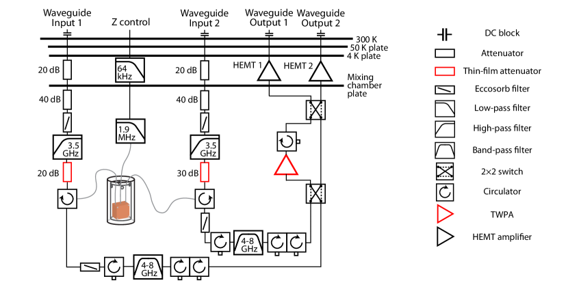
The measurement setup inside the dilution refrigerator is illustrated in Fig. 10. All the 14 qubits on Device I are DC-biased with individual flux-bias (Z control) lines, filtered by a 64 kHz low-pass filter at the 4K plate and a 1.9 MHz low-pass filter at the mixing chamber plate. The Waveguide Input 1 (2) passes through a series of attenuators and filters including a 20 dB (30 dB) thin-film attenuator developed in B. Palmer’s group Yeh et al. (2017). It connects via a circulator to port 1 (2) of Device I, which is enclosed in two layers of magnetic shielding. The output signals from Device I are routed by the same circulator to the output lines containing a series of circulators and filters. The pair of 22 switches in the amplification chain allows us to choose the branch to be further amplified in the first stage by a traveling-wave parametric amplifier (TWPA) from MIT Lincoln Laboratories. Both of the output lines are amplified by an individual high electron mobility transistor (HEMT) at the 4K plate, followed by room-temperature amplifiers at 300 K. All four S-parameters () involving port 1 and 2 on Device I can be measured with this setup by choosing one of the waveguide input ports and one of the waveguide output ports, e.g. can be measured by sending the input signal into Waveguide Input 1 and collecting the output signal from Waveguide Output 2 with both 22 switches in the cross () configuration.
Appendix D Tapering sections on Device I
The finite system size of metamaterial waveguide gives rise to sharp resonances inside the passband associated with reflection at the boundary (Fig. 1d of the main text). Also, the decay rate of qubits to external ports inside the middle bandgap (MBG) is small, making the spectroscopic measurement of qubits inside the MBG hard to achieve. In order to reduce ripples in transmission spectrum inside the upper passband and increase the decay rates of qubits to external ports comparable to their intrinsic contributions inside the middle bandgap, we added two resonators at each end of the metamaterial waveguide in Device I as tapering section.
Similar to the procedure described in Appendix C of Ref. Ferreira et al. (2020), the idea is to increase the coupling capacitance gradually across the two resonators while keeping the resonator frequency the same as other resonators by changing the self capacitance as well. However, unlike the simple case of an array of LC resonators with uniform coupling capacitance, the SSH waveguide consists of alternating coupling capacitance between neighboring resonators and two separate passbands form as a result. In this particular work, the passband experiments are designed to take place at the upper passband frequencies and hence we have slightly modified the resonant frequencies of tapering resonators to perform impedance-matching inside the upper passband. The circuit diagram shown in Fig. 11a was used to model the tapering section in our system. While designing of tapering sections involves empirical trials, microwave filter design software, e.g. iFilter module in AWR Microwave Office iFi , can be used to aid the choice of circuit parameters and optimization method.
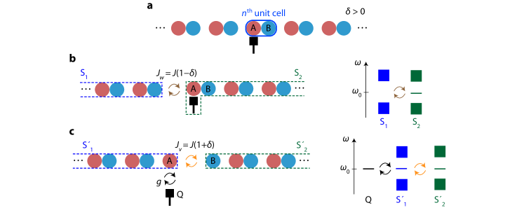
Figure 11b shows the optical micrograph of a tapering section on Device I. The circuit parameters are extracted by fitting the normalized waveguide transmission spectrum () data from measurement with theoretical circuit models. We find a good agreement in the frequency of normal modes and the level of ripples between the theoretical model and the experiment as illustrated in Fig. 11c. The level of ripples in the transmission spectrum of the entire upper passband is about 8 dB and decreases to below 2 dB near the center of the band, allowing us to probe the cooperative interaction between qubits at these frequencies.
Appendix E Directional shape of qubit-photon bound state
In this section, we provide detailed explanations on the directional shape of qubit-photon bound states discussed in the main text. As an example, we consider a system consisting of a topological waveguide in the trivial phase and a qubit coupled to the A sublattice of the -th unit cell (Fig. 12a). Our descriptions are based on partitioning the system into subsystems under two alternative pictures (Fig. 12b,c), where the array is divided on the left (Description I) or the right (Description II) of the site where the qubit is coupled to.
E.1 Description I
We divide the array into two parts by breaking the inter-cell coupling that exists on the left of the site where the qubit is coupled to, i.e., between sites and . The system is described in terms of two subsystems S1 and S2 as shown in Fig. 12b. The subsystem S1 is a semi-infinite array in the trivial phase extended from the -th unit cell to the left and the subsystem S2 comprising a qubit and a semi-infinite array in the trivial phase extended from the -th unit cell to the right. The coupling between the two subsystems is interpreted to take place at a boundary site with coupling strength . When the qubit frequency is resonant to the reference frequency , the subsystem S2 can be viewed as a semi-infinite array in the topological phase, where the qubit effectively acts as an edge site. Here, the resulting topological edge mode of subsystem S2 is the qubit-photon bound state, with photon occupation mostly on the qubit itself and on every B site with a decaying envelope. Coupling of subsystem S2 to S1 only has a minor effect on the edge mode of S2 as the modes in subsystem S1 are concentrated at passband frequencies, far-detuned from . Also, the presence of an edge state of S2 at cannot induce an additional occupation on S1 by this coupling in a way that resembles an edge state since the edge mode of S2 does not occupy sites on the A sublattice. The passband modes S1 and S2 near-resonantly couple to each other, whose net effect is redistribution of modes within the passband frequencies. Therefore, the qubit-photon bound state can be viewed as a topological edge mode for subsystem S2 which is unperturbed by coupling to subsystem S1. The directionality and photon occupation distribution along the resonator chain of the qubit-photon bound state can be naturally explained according to this picture.
E.2 Description II
In this alternate description, we divide the array into two parts by breaking the intra-cell coupling that exists on the right of the site where the qubit is coupled to, i.e., between sites and . We consider the division of the system into three parts: the qubit, subsystem S, and subsystem S as illustrated in Fig. 12c. Here, the subsystem S (S) is a semi-infinite array in the topological phase extended to the left (right), where the last site hosting the topological edge mode E (E) at is the A (B) sublattice of the -th unit cell. The subsystem S is coupled to both the qubit and the subsystem S with coupling strength and , respectively. Similar to Description I, the result of coupling between subsystem modes inside the passband is the reorganization of modes without significant change in the spectrum inside the middle bandgap. On the other hand, modes of the subsystems at (qubit, E, and E) can be viewed as emitters coupled in a linear chain configuration, whose eigenfrequencies and corresponding eigenstates in the single-excitation manifold are given by
and
where denotes a state with photons in the (qubit, E, E), respectively. Here, () is the coupling between edge mode E and the qubit (edge mode E), diluted from () due to the admixture of photonic occupation on sites other than the boundary in the edge modes. Note that in the limit of short localization length, we recover and . Among the three single-excitation eigenstates, the states lie at frequencies of approximately , and are absorbed into the passbands. The only remaining state inside the middle bandgap is the state , existing exactly at , which is an anti-symmetric superposition of qubit excited state and the single-photon state of E, whose photonic envelope is directed to the right with occupation on every B site. This accounts for the directional qubit-photon bound state emerging in this scenario.
Appendix F Coupling of qubit-photon bound states to external ports at different frequencies
As noted in the main text (Fig. 2), the perfect directionality of the qubit-photon bound states is achieved only at the reference frequency inside the middle bandgap. In this section, we discuss the breakdown of the observed perfect directionality when qubits are tuned to different frequencies inside the middle bandgap by showing the behavior of the external coupling () to the ports.
F.1 Inside the middle bandgap, detuned from the reference frequency
Figure 13a shows the external coupling rate of qubits to the ports at 6.72 GHz, a frequency in the middle bandgap close to band-edge. The alternating behavior of external coupling rate is still observed, but with a smaller contrast than in Fig. 2 of the main text. The dependence of external linewidth on qubit index still exhibits the remaining directionality with qubits on A (B) sublattice maintaining large coupling to port 2 (1), while showing small non-zero coupling to the opposite port.
F.2 Inside the upper bandgap
Inside the upper bandgap (7.485 GHz), the coupling of qubit-photon bound states to external ports decreases monotonically with the distance of the qubit site to the port, regardless of which sublattice the qubit is coupled to (Fig. 13b). This behavior is similar to that of qubit-photon bound states formed in a structure with uniform coupling, where bound states exhibit a symmetric photonic envelope surrounding the qubit. Note that we find the external coupling to port 2 () to be generally smaller than that to port 1 (), which may arise from a slight impedance mismatch on the connection of the device to the external wiring.
Appendix G Probing band topology with qubits
G.1 Signature of perfect super-radiance
Here we take a closer look at the swirl pattern in the waveguide transmission spectrum – a signature of perfect super-radiance – which is discussed in Fig. 3c of the main text. In Fig. 14 we zoom in to the observed swirl pattern near 6.95 GHz, and three horizontal line cuts. At the center of this pattern (sub-panel ii. of Fig. 14b), the two qubits form perfect super-/sub-radiant states with maximized correlated decay and zero coherent exchange interaction van Loo et al. (2013); Lalumière et al. (2013). At this point, the transmission spectrum shows a single Lorentzian lineshape (perfect super-radiant state and bright state) with linewidth equal to the sum of individual linewidths of the coupled qubits. The perfect sub-radiant state (dark state), which has no external coupling, cannot be accessed from the waveguide channel here and is absent in the spectrum. Slightly away from this frequency, the coherent exchange interaction starts to show up, making hybridized states , formed by the interaction of the two qubits. In this case, both of the hybridized states have non-zero decay rate to the waveguide, forming a V-type level structure Bello et al. (2019). The interference between photons scattering off the two hybridized states gives rise to the peak in the middle of sub-panels (i.) and (iii.) in Fig. 14b.
The fitting of lineshapes starts with the subtraction of transmission spectrum of the background, which are taken in the same frequency window but with qubits detuned away. Note that the background subtraction in this case cannot be perfect due to the frequency shift of the upper passband modes under the presence of qubits. Such imperfection accounts for most of the discrepancy between the fit and the experimental data. The fit employs the transfer matrix method discussed in Refs. van Loo (2014); Shen and Fan (2005a, b). Here, the transfer matrix of the two qubits takes into account the pure dephasing, which causes the sharp peaks in sub-panels (i.) and (iii.) of Fig. 14b to stay below perfect transmission level (unity) as opposed to the prediction from the ideal case of electromagnetically induced transparency Witthaut and Sorensen (2010).
G.2 Topology-dependent photon scattering on various qubit pairs
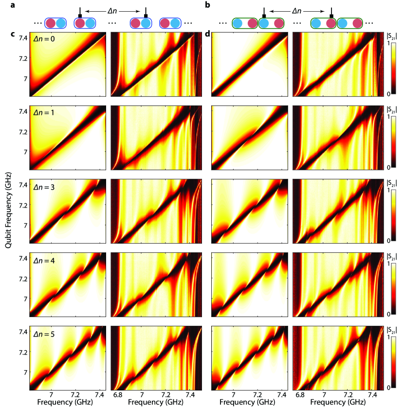
As mentioned in the main text, when the two qubits are separated by () unit cells, perfect super-radiance (vanishing of coherent exchange interaction) takes place exactly times in the trivial phase and times in the topological phase across the entire passband. The main text shows the case of . Here we report similar measurements on other qubit pairs with different cell distance between the qubits. Figure 15 shows good qualitative agreement between the experiment and theoretical result in Ref. Bello et al. (2019). The small avoided-crossing-like features in the experimental data are due to coupling of one of the qubits with a local two-level system defect. An example of this is seen near 6.85 GHz of in the topological configuration. For , there is no perfect super-radiant point throughout the passband for both trivial and topological configurations. For all the other combinations in Fig. 15, the number of swirl patterns indicating perfect super-radiance agrees with the theoretical model.
[t] Qubit (GHz) (MHz) (GHz) (MHz) (GHz) (MHz) (s) (s) 8.23 294 30.89 58.1 5.30 43.5 4.73 4.04 7.99 296 28.98 57.3 5.39 43.4 13.9 8.3
Appendix H Device II characterization and experimental setup
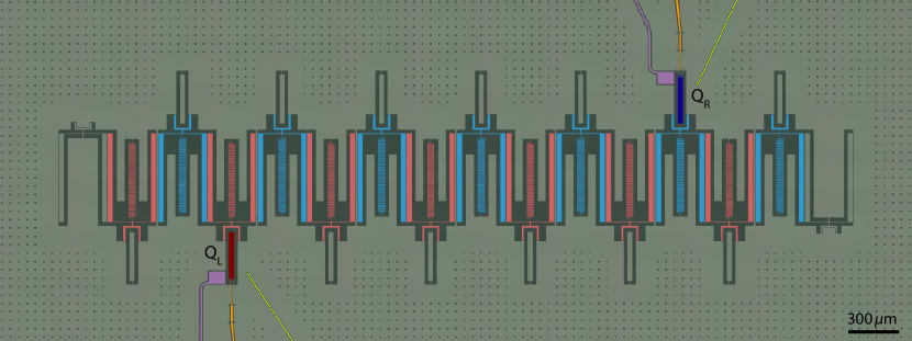
In this section we provide a detailed description of the elements making up Device II, in which the edge mode experiments are performed. The optical micrograph of Device II is illustrated in Fig. 16.
H.1 Qubits
The parameters of qubits on Device II are summarized in Table 2. The two qubits are designed to have identical SQUID loops with symmetric JJs. The lifetime and Ramsey coherence times in the table are measured when qubits are tuned to their sweet spot. Qubit coherence at the working frequency in the middle bandgap is also characterized, with the lifetime and Ramsey coherence times of () at 6.829 (6.835) GHz measured to be (5.803) s and (539) ns, respectively.
H.2 Metamaterial waveguide and coupling to qubits
The resonators in the metamaterial waveguide and their coupling to qubits are designed to be nominally identical to those in Device I. The last resonators of the array are terminated with a wing-shape patterned ground plane region in order to maintain the bare self-capacitance identical to other resonators.
H.3 Edge modes
The coherence of the edge modes is characterized by using qubits to control and measure the excitation with single-photon precision. Taking as an example, we define the iSWAP gate as a half-cycle of the vacuum Rabi oscillation in Fig. 4d of the main text. For measurement of the lifetime of the edge state E, the qubit Q is initially prepared in its excited state with a microwave -pulse, and an iSWAP gate is applied to transfer the population from to . After waiting for a variable delay, we perform the second iSWAP to retrieve the population from back to , followed by the readout of . In order to measure the Ramsey coherence time, the qubit Q is instead prepared in an equal superposition of ground and excited states with a microwave -pulse, followed by an iSWAP gate. After a variable delay, we perform the second iSWAP and another -pulse on Q, followed by the readout of . An equivalent pulse sequence for Q is used to characterize the coherence of E. The lifetime and Ramsey coherence time of () are extracted to be (2.96) s and (2.91) s, respectively, when () is parked at 6.829 (6.835) GHz. Due to the considerable amount of coupling between the qubit and the edge mode compared to the detuning at park frequency, the edge modes are hybridized with the qubits during the delay time in the above-mentioned pulse sequences. As a result, the measured coherence time of the edge modes is likely limited here by the dephasing of the qubits.
H.4 Experimental setup
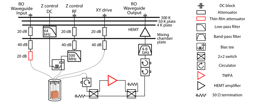
The measurement setup inside the dilution refrigerator is illustrated in Fig. 17. The excitation of the two qubits is controlled by capacitively-coupled individual XY microwave drive lines. The frequency of qubits are controlled by individual DC bias (Z control DC) and RF signals (Z control RF), which are combined using a bias tee at the mixing chamber plate. The readout signals are sent into RO Waveguide Input, passing through a series of attenuators including a 20 dB thin-film attenuator developed in B. Palmer’s group Yeh et al. (2017). The output signals go through an optional TWPA, a series of circulators and a band-pass filter, which are then amplified by a HEMT amplifier (RO Waveguide Output).
H.5 Details on the population transfer process
In step i) of the double-modulation scheme described in the main text, the frequency modulation pulse on (control modulation) is set to be 2 ns longer than that on (transfer modulation). The interaction strength induced by the control modulation is 21.1 MHz, smaller than that induced by the transfer modulation in order to decrease the population leakage between the two edge states. For step iii), the interaction strength induced by the control modulation on is 22.4 MHz, much closer to interaction strength for the transfer than expected (this was due to a poor calibration of the modulation efficiency of qubit sideband). The interaction strengths being too close between and gives rise to unwanted leakage and decreases the required interaction time in step ii). We expect that a careful optimization on the frequency modulation pulses would have better addressed this leakage problem and increase the transfer fidelity (see below).
The fit to the curves in Fig. 4e of the main text are based on numerical simulation with QuTiP Johansson et al. (2012, 2013), assuming the values of lifetime () and coherence time () from the characterization measurements. The free parameters in the simulation are the coupling strengths , between qubits and edge states, whose values are extracted from the best fit of the experimental data.
The detailed contributions to the infidelity of the as-implemented population transfer protocol are also analyzed by utilizing QuTiP. The initial left-side qubit population probability is measured to be only 98.4 %, corresponding to an infidelity of 1.6 % in the -pulse qubit excitation in this transfer experiment (compared to a previously calibrated ‘optimized’ pulse). In the following steps, we remove the leakage between edge modes and the decoherence process sequentially to see their individual contributions to infidelity. First, we set the coupling strength between the two edge modes to zero during the two iSWAP gates while keeping the above-mentioned initial population probability, coupling strengths, lifetimes, and coherence times. The elimination of unintended leakage during the left and right side iSWAP steps between the edge modes gives the final transferred population probability of 91.9 %, suggesting of the infidelity comes from the unintended leakage between edge modes. Also, as expected, setting the population decay and decoherence of the qubits and the edge modes to zero, the final population is found to be identical to the initial value, indicating that of loss arises from the decoherence processes.
References
- Haldane and Raghu (2008) F. Haldane and S. Raghu, Possible realization of directional optical waveguides in photonic crystals with broken time-reversal symmetry, Phys. Rev. Lett. 100, 013904 (2008).
- Lu et al. (2014) L. Lu, J. D. Joannopoulos, and M. Soljačić, Topological photonics, Nat. Photonics 8, 821 (2014).
- Ozawa et al. (2019) T. Ozawa, H. M. Price, A. Amo, N. Goldman, M. Hafezi, L. Lu, M. C. Rechtsman, D. Schuster, J. Simon, O. Zilberberg, and I. Carusotto, Topological photonics, Rev. Mod. Phys. 91, 015006 (2019).
- von Klitzing (1986) K. von Klitzing, The quantized Hall effect, Rev. Mod. Phys. 58, 519 (1986).
- Hasan and Kane (2010) M. Z. Hasan and C. L. Kane, Colloquium: Topological insulators, Rev. Mod. Phys. 82, 3045 (2010).
- Chen et al. (2013) X. Chen, Z.-C. Gu, Z.-X. Liu, and X.-G. Wen, Symmetry protected topological orders and the group cohomology of their symmetry group, Phys. Rev. B 87, 155114 (2013).
- Smirnova et al. (2019) D. Smirnova, D. Leykam, Y. Chong, and Y. Kivshar, Nonlinear topological photonics, arXiv:1912.01784 (2019).
- Su et al. (1979) W. P. Su, J. R. Schrieffer, and A. J. Heeger, Solitons in Polyacetylene, Phys. Rev. Lett. 42, 1698 (1979).
- Asbóth et al. (2016) J. K. Asbóth, L. Oroszlány, and A. Pályi, A Short Course on Topological Insulators, Lecture Notes in Physics (Springer, 2016).
- St-Jean et al. (2017) P. St-Jean, V. Goblot, E. Galopin, A. Lemaître, T. Ozawa, L. L. Gratiet, I. Sagnes, J. Bloch, and A. Amo, Lasing in topological edge states of a one-dimensional lattice, Nat. Photonics 11, 651 (2017).
- Zhao et al. (2018) H. Zhao, P. Miao, M. H. Teimourpour, S. Malzard, R. El-Ganainy, H. Schomerus, and L. Feng, Topological hybrid silicon microlasers, Nat. Commun. 9, 981 (2018).
- Ota et al. (2018) Y. Ota, R. Katsumi, K. Watanabe, S. Iwamoto, and Y. Arakawa, Topological photonic crystal nanocavity laser, Commun. Phys. 1, 86 (2018).
- Kruk et al. (2019) S. Kruk, A. Poddubny, D. Smirnova, L. Wang, A. Slobozhanyuk, A. Shorokhov, I. Kravchenko, B. Luther-Davies, and Y. Kivshar, Nonlinear light generation in topological nanostructures, Nat. Nanotechnol. 14, 126 (2019).
- Carusotto and Ciuti (2013) I. Carusotto and C. Ciuti, Quantum fluids of light, Rev. Mod. Phys. 85, 299 (2013).
- Cai et al. (2019) W. Cai, J. Han, F. Mei, Y. Xu, Y. Ma, X. Li, H. Wang, Y. Song, Z.-Y. Xue, Z.-q. Yin, et al., Observation of topological magnon insulator states in a superconducting circuit, Phys. Rev. Lett. 123, 080501 (2019).
- de Léséleuc et al. (2019) S. de Léséleuc, V. Lienhard, P. Scholl, D. Barredo, S. Weber, N. Lang, H. P. Büchler, T. Lahaye, and A. Browaeys, Observation of a symmetry-protected topological phase of interacting bosons with Rydberg atoms, Science 365, 775 (2019).
- Haroche and Raimond (2006) S. Haroche and J.-M. Raimond, Exploring the quantum: atoms, cavities, and photons (Oxford University Press, 2006).
- Lodahl et al. (2015) P. Lodahl, S. Mahmoodian, and S. Stobbe, Interfacing single photons and single quantum dots with photonic nanostructures, Rev. Mod. Phys. 87, 347 (2015).
- Chang et al. (2018) D. E. Chang, J. S. Douglas, A. González-Tudela, C.-L. Hung, and H. J. Kimble, Colloquium: Quantum matter built from nanoscopic lattices of atoms and photons, Rev. Mod. Phys. 90, 031002 (2018).
- Douglas et al. (2015) J. S. Douglas, H. Habibian, C.-L. Hung, A. V. Gorshkov, H. J. Kimble, and D. E. Chang, Quantum many-body models with cold atoms coupled to photonic crystals, Nat. Photonics 9, 326 (2015).
- Shi et al. (2018) T. Shi, Y. H. Wu, A. González-Tudela, and J. I. Cirac, Effective many-body Hamiltonians of qubit-photon bound states, New J. Phys. 20, 105005 (2018).
- Liu and Houck (2016) Y. Liu and A. A. Houck, Quantum electrodynamics near a photonic bandgap, Nat. Phys. 13, 48 (2016).
- Hung et al. (2016) C. L. Hung, A. González-Tudela, J. I. Cirac, and H. J. Kimble, Quantum spin dynamics with pairwise-tunable, long-range interactions, Proc. Natl. Acad. Sci. U.S.A 113, E4946 (2016).
- Barik et al. (2018) S. Barik, A. Karasahin, C. Flower, T. Cai, H. Miyake, W. DeGottardi, M. Hafezi, and E. Waks, A topological quantum optics interface, Science 359, 666 (2018).
- Lodahl et al. (2017) P. Lodahl, S. Mahmoodian, S. Stobbe, A. Rauschenbeutel, P. Schneeweiss, J. Volz, H. Pichler, and P. Zoller, Chiral quantum optics, Nature 541, 473 (2017).
- Bello et al. (2019) M. Bello, G. Platero, J. I. Cirac, and A. González-Tudela, Unconventional quantum optics in topological waveguide QED, Sci. Adv. 5, eaaw0297 (2019).
- García-Elcano et al. (2019) I. García-Elcano, A. González-Tudela, and J. Bravo-Abad, Quantum electrodynamics near photonic Weyl points (2019), arXiv:1903.07513 .
- Koch et al. (2007) J. Koch, T. M. Yu, J. Gambetta, A. A. Houck, D. I. Schuster, J. Majer, A. Blais, M. H. Devoret, S. M. Girvin, and R. J. Schoelkopf, Charge-insensitive qubit design derived from the Cooper pair box, Phys. Rev. A 76, 042319 (2007).
- Mirhosseini et al. (2018) M. Mirhosseini, E. Kim, V. S. Ferreira, M. Kalaee, A. Sipahigil, A. J. Keller, and O. Painter, Superconducting metamaterials for waveguide quantum electrodynamics, Nat. Commun. 9, 3706 (2018).
- Ferreira et al. (2020) V. S. Ferreira, J. Banker, A. Sipahigil, M. H. Matheny, A. J. Keller, E. Kim, M. Mirhosseini, and O. Painter, Collapse and Revival of an Artificial Atom Coupled to a Structured Photonic Reservoir (2020), arXiv:2001.03240 .
- Gu et al. (2017) X. Gu, A. F. Kockum, A. Miranowicz, Y.-x. Liu, and F. Nori, Microwave photonics with superconducting quantum circuits, Phys. Rep. 718-719, 1 (2017).
- Roy et al. (2017) D. Roy, C. M. Wilson, and O. Firstenberg, Colloquium: Strongly interacting photons in one-dimensional continuum, Rev. Mod. Phys. 89, 021001 (2017).
- Zak (1989) J. Zak, Berry’s phase for energy bands in solids, Phys. Rev. Lett. 62, 2747 (1989).
- John and Wang (1990) S. John and J. Wang, Quantum electrodynamics near a photonic band gap: Photon bound states and dressed atoms, Phys. Rev. Lett. 64, 2418 (1990).
- Kurizki (1990) G. Kurizki, Two-atom resonant radiative coupling in photonic band structures, Phys. Rev. A 42, 2915 (1990).
- Biondi et al. (2014) M. Biondi, S. Schmidt, G. Blatter, and H. E. Türeci, Self-protected polariton states in photonic quantum metamaterials, Phys. Rev. A 89, 025801 (2014).
- Chang et al. (2012) D. E. Chang, L. Jiang, A. V. Gorshkov, and H. J. Kimble, Cavity QED with atomic mirrors, New J. Phys. 14, 063003 (2012).
- Lalumière et al. (2013) K. Lalumière, B. C. Sanders, A. F. van Loo, A. Fedorov, A. Wallraff, and A. Blais, Input-output theory for waveguide QED with an ensemble of inhomogeneous atoms, Phys. Rev. A 88, 043806 (2013).
- Dicke (1954) R. H. Dicke, Coherence in Spontaneous Radiation Processes, Phys. Rev. 93, 99 (1954).
- Witthaut and Sorensen (2010) D. Witthaut and A. S. Sorensen, Photon scattering by a three-level emitter in a one-dimensional waveguide, New J. Phys. 12, 043052 (2010).
- Naik et al. (2017) R. K. Naik, N. Leung, S. Chakram, P. Groszkowski, Y. Lu, N. Earnest, D. C. McKay, J. Koch, and D. I. Schuster, Random access quantum information processors using multimode circuit quantum electrodynamics, Nat. Commun. 8, 1904 (2017).
- Chen et al. (2012) Y. Chen, D. Sank, P. O’Malley, T. White, R. Barends, B. Chiaro, J. Kelly, E. Lucero, M. Mariantoni, A. Megrant, C. Neill, A. Vainsencher, J. Wenner, Y. Yin, A. N. Cleland, and J. M. Martinis, Multiplexed dispersive readout of superconducting phase qubits, Appl. Phys. Lett. 101, 182601 (2012).
- Khaneja et al. (2005) N. Khaneja, T. Reiss, C. Kehlet, T. Schulte-Herbrüggen, and S. J. Glaser, Optimal control of coupled spin dynamics: design of NMR pulse sequences by gradient ascent algorithms, J. Magn. Reson. 172, 296 (2005).
- Motzoi et al. (2009) F. Motzoi, J. M. Gambetta, P. Rebentrost, and F. K. Wilhelm, Simple Pulses for Elimination of Leakage in Weakly Nonlinear Qubits, Phys. Rev. Lett. 103, 110501 (2009).
- Didier et al. (2018) N. Didier, E. A. Sete, J. Combes, and M. P. d. Silva, AC flux sweet spots in parametrically-modulated superconducting qubits, Phys. Rev. Appl. 12, 054015 (2018).
- Hong et al. (2020) S. S. Hong, A. T. Papageorge, P. Sivarajah, G. Crossman, N. Didier, A. M. Polloreno, E. A. Sete, S. W. Turkowski, M. P. d. Silva, and B. R. Johnson, Demonstration of a parametrically activated entangling gate protected from flux noise, Phys. Rev. A 101, 012302 (2020).
- Sete et al. (2017) E. A. Sete, M. J. Reagor, N. Didier, and C. T. Rigetti, Charge- and Flux-Insensitive Tunable Superconducting Qubit, Phys. Rev. Appl. 8, 024004 (2017).
- Hutchings et al. (2017) M. D. Hutchings, J. B. Hertzberg, Y. Liu, N. T. Bronn, G. A. Keefe, M. Brink, J. M. Chow, and B. L. T. Plourde, Tunable Superconducting Qubits with Flux-Independent Coherence, Phys. Rev. Appl. 8, 044003 (2017).
- Ott (2009) H. W. Ott, Electromagnetic Compatibility Engineering (John Wiley & Sons, Inc., 2009).
- Chen et al. (2014) Y. Chen, C. Neill, P. Roushan, N. Leung, M. Fang, R. Barends, J. Kelly, B. Campbell, Z. Chen, B. Chiaro, A. Dunsworth, E. Jeffrey, A. Megrant, J. Y. Mutus, P. J. J. O’Malley, C. M. Quintana, D. Sank, A. Vainsencher, J. Wenner, T. C. White, M. R. Geller, A. N. Cleland, and J. M. Martinis, Qubit Architecture with High Coherence and Fast Tunable Coupling, Phys. Rev. Lett. 113, 220502 (2014).
- Lang and Büchler (2017) N. Lang and H. P. Büchler, Topological networks for quantum communication between distant qubits, npj Quantum Inf. 3, 47 (2017).
- Kimble (2008) H. J. Kimble, The quantum internet, Nature 453, 1023 (2008).
- Tran et al. (2017) D. T. Tran, A. Dauphin, A. G. Grushin, P. Zoller, and N. Goldman, Probing topology by “heating”: Quantized circular dichroism in ultracold atoms, Sci. Adv. 3, e1701207 (2017).
- Dunsworth et al. (2018) A. Dunsworth, R. Barends, Y. Chen, Z. Chen, B. Chiaro, A. Fowler, B. Foxen, E. Jeffrey, J. Kelly, P. V. Klimov, E. Lucero, J. Y. Mutus, M. Neeley, C. Neill, C. Quintana, P. Roushan, D. Sank, A. Vainsencher, J. Wenner, T. C. White, H. Neven, J. M. Martinis, and A. Megrant, A method for building low loss multi-layer wiring for superconducting microwave devices, Appl. Phys. Lett. 112, 063502 (2018).
- Rosenberg et al. (2017) D. Rosenberg, D. Kim, R. Das, D. Yost, S. Gustavsson, D. Hover, P. Krantz, A. Melville, L. Racz, G. O. Samach, S. J. Weber, F. Yan, J. Yoder, A. J. Kerman, and W. D. Oliver, 3D integrated superconducting qubits, npj Quantum Inf. 3, 42 (2017).
- Foxen et al. (2017) B. Foxen, J. Y. Mutus, E. Lucero, R. Graff, A. Megrant, Y. Chen, C. Quintana, B. Burkett, J. Kelly, E. Jeffrey, Y. Yang, A. Yu, K. Arya, R. Barends, Z. Chen, B. Chiaro, A. Dunsworth, A. Fowler, C. Gidney, M. Giustina, T. Huang, P. Klimov, M. Neeley, C. Neill, P. Roushan, D. Sank, A. Vainsencher, J. Wenner, T. C. White, and J. M. Martinis, Qubit compatible superconducting interconnects, Quantum Sci. Technol. 3, 014005 (2017).
- Jeffrey et al. (2014) E. Jeffrey, D. Sank, J. Y. Mutus, T. C. White, J. Kelly, R. Barends, Y. Chen, Z. Chen, B. Chiaro, A. Dunsworth, A. Megrant, P. J. J. O’Malley, C. Neill, P. Roushan, A. Vainsencher, J. Wenner, A. N. Cleland, and J. M. Martinis, Fast Accurate State Measurement with Superconducting Qubits, Phys. Rev. Lett. 112, 190504 (2014).
- Ma et al. (2017) R. Ma, C. Owens, A. Houck, D. I. Schuster, and J. Simon, Autonomous stabilizer for incompressible photon fluids and solids, Phys. Rev. A 95, 043811 (2017).
- Ma et al. (2019) R. Ma, B. Saxberg, C. Owens, N. Leung, Y. Lu, J. Simon, and D. I. Schuster, A dissipatively stabilized Mott insulator of photons, Nature 566, 51 (2019).
- Krantz et al. (2019) P. Krantz, M. Kjaergaard, F. Yan, T. P. Orlando, S. Gustavsson, and W. D. Oliver, A quantum engineer’s guide to superconducting qubits, Appl. Phys. Rev. 6, 021318 (2019).
- Anderson et al. (2016) B. M. Anderson, R. Ma, C. Owens, D. I. Schuster, and J. Simon, Engineering Topological Many-Body Materials in Microwave Cavity Arrays, Phys. Rev. X 6, 041043 (2016).
- Owens et al. (2018) C. Owens, A. LaChapelle, B. Saxberg, B. M. Anderson, R. Ma, J. Simon, and D. I. Schuster, Quarter-flux Hofstadter lattice in a qubit-compatible microwave cavity array, Phys. Rev. A 97, 013818 (2018).
- Blatt and Roos (2012) R. Blatt and C. F. Roos, Quantum simulations with trapped ions, Nat. Phys. 8, 277 (2012).
- Gross and Bloch (2017) C. Gross and I. Bloch, Quantum simulations with ultracold atoms in optical lattices, Science 357, 995 (2017).
- Lewis-Swan et al. (2019) R. J. Lewis-Swan, A. Safavi-Naini, A. M. Kaufman, and A. M. Rey, Dynamics of quantum information, Nat. Rev. Phys. 1, 627 (2019).
- Georgescu et al. (2014) I. M. Georgescu, S. Ashhab, and F. Nori, Quantum simulation, Rev. Mod. Phys. 86, 153 (2014).
- Carusotto et al. (2020) I. Carusotto, A. A. Houck, A. J. Kollár, P. Roushan, D. I. Schuster, and J. Simon, Photonic materials in circuit quantum electrodynamics, Nat. Phys. 16, 268 (2020).
- Goren et al. (2018) T. Goren, K. Plekhanov, F. Appas, and K. L. Hur, Topological Zak phase in strongly coupled LC circuits, Phys. Rev. B 97, 041106 (2018).
- Kockum et al. (2019) A. F. Kockum, A. Miranowicz, S. D. Liberato, S. Savasta, and F. Nori, Ultrastrong coupling between light and matter, Nat. Rev. Phys. 1, 19 (2019).
- Pérez-González et al. (2018) B. Pérez-González, M. Bello, A. Gómez-León, and G. Platero, SSH model with long-range hoppings: topology, driving and disorder, arXiv:1802.03973v3 (2018).
- Longhi (2018) S. Longhi, Probing one-dimensional topological phases in waveguide lattices with broken chiral symmetry, Opt. Lett. 43, 4639 (2018).
- Mirhosseini et al. (2019) M. Mirhosseini, E. Kim, X. Zhang, A. Sipahigil, P. B. Dieterle, A. J. Keller, A. Asenjo-Garcia, D. E. Chang, and O. Painter, Cavity quantum electrodynamics with atom-like mirrors, Nature 569, 692 (2019).
- Sank (2014) D. T. Sank, Fast, Accurate State Measurement in Superconducting Qubits, Ph.D. thesis, UC Santa Barbara (2014).
- Yeh et al. (2017) J.-H. Yeh, J. LeFebvre, S. Premaratne, F. Wellstood, and B. Palmer, Microwave attenuators for use with quantum devices below 100 mK, J. Appl. Phys. 121, 224501 (2017).
- (75) iFilter™ Module, AWR Design Environment, https://www.awr.com/software/options/ifilter.
- van Loo et al. (2013) A. F. van Loo, A. Fedorov, K. Lalumière, B. C. Sanders, A. Blais, and A. Wallraff, Photon-Mediated Interactions Between Distant Artificial Atoms, Science 342, 1494 (2013).
- van Loo (2014) A. F. van Loo, Interactions in waveguide quantum electrodynamics, Ph.D. thesis, ETH Zurich (2014).
- Shen and Fan (2005a) J.-T. Shen and S. Fan, Coherent photon transport from spontaneous emission in one-dimensional waveguides, Opt. Lett. 30, 2001 (2005a).
- Shen and Fan (2005b) J.-T. Shen and S. Fan, Coherent single photon transport in a one-dimensional waveguide coupled with superconducting quantum bits, Phys. Rev. Lett. 95, 213001 (2005b).
- Johansson et al. (2012) J. R. Johansson, P. D. Nation, and F. Nori, QuTiP: An open-source Python framework for the dynamics of open quantum systems, Comput. Phys. Commun. 183, 1760 (2012).
- Johansson et al. (2013) J. R. Johansson, P. D. Nation, and F. Nori, QuTiP 2: A Python framework for the dynamics of open quantum systems, Comput. Phys. Commun. 184, 1234 (2013).