Quantum criticality at finite temperature for two-dimensional models on the square and the honeycomb lattices
Abstract
We study the quantum criticality at finite temperature for three two-dimensional (2D) models using the first principle nonperturbative quantum Monte Carlo calculations (QMC). In particular, the associated universal quantities are obtained and their inverse temperature dependence are investigated. The considered models are known to have quantum phase transitions from the Néel order to the valence bond solid. In addition, these transitions are shown to be of second order for two of the studied models, with the remaining one being of first order. Interestingly, we find that the outcomes obtained in our investigation are consistent with the mentioned scenarios regarding the nature of the phase transitions of the three investigated models. Moreover, when the temperature dependence of the studied universal quantities is considered, a substantial difference between the two models possessing second order phase transitions and the remaining model is observed. Remarkably, by using the associated data from both the models that may have continuous transitions, good data collapses are obtained for a number of the considered universal quantities. The findings presented here not only provide numerical evidence to support the results established in the literature regarding the nature of the phase transitions of these models, but also can be employed as certain promising criterions to distinguish second order phase transitions from first order ones for the exotic criticalities of the -type models. Finally, based on a comparison between the results calculated here and the corresponding theoretical predictions, we conclude that a more detailed analytic calculation is required in order to fully catch the numerical outcomes determined in our investigation.
I Introduction
Studying the characteristics of transitions between various phases of matters has long been an active research topic in the condensed matter physics Nig92 ; Car96 ; Car10 ; Sac11 . In particular, with the advances of experimental techniques and theoretical approaches, some exotic phases and (or) abnormal transitions between various states are observed and (or) proposed. One such a noticeable example is the transition between the Néel phase and the valence bond solid San07 .
The so-called -type models of (quantum) spins in two-dimension (2D) San07 ; Lou09 ; Sen10 , which will be introduced later, are systems hosting the exotic phase transition between the Néel and the valence bond solid states. The models have two types of couplings, namely the -term and the -term. In addition, when the magnitudes of the couplings increase, the -term and the -term favor the formation of singlets and pairs of singlets (valence bond solid, VBS), respectively. On the one hand, when the magnitude of is much smaller than that of , the symmetry is broken spontaneously and the system is in the antiferromagnetic long-range order. On the other hand, the translation symmetry is broken in the case of . If one starts with a value of ( and is fixed to be 1) so that the long-range order exists and the translation symmetry of the system is unbroken, then by increasing the magnitude of one expects that the restoration of the broken symmetry and the breaking of the translation symmetry should occur at some couplings . In particular, these two distinct physical incidents may take place at different values of . If the two mentioned transitions occur at the same , which is the most interesting scenario, then without fine-tuning this phase transition should be first order according to the famous Landau-Ginsburg paradigm Gin50 .
Although the intriguing exotic phase transition introduced in the previous paragraph should be first order in general, it is argue theoretically that this phase transition, as well as those which belong to some other models possessing similar characteristics of the -type models, can be second order Sen040 ; Sen041 . Such an exotic critical behavior is referred to as the deconfined quantum criticality (DQC) in the literature.
Many numerical investigations have been carried out in order to understand DQC, and various conclusions are obtained Kuk06 ; Mel07 ; Jia08 ; Kuk08 ; San10 ; Che13 ; Har13 . Although consistent critical exponents are obtained by simulating square lattices as large as 4482 Sha16 ; San201 , one still cannot rule out the possibility that the considered phase transition of the model (on the square lattice) is a weakly first order one. Indeed, it is shown in Ref. Iin19 that while the phase transition of the ferromagnetic 5-state Potts model on the square lattice is a weakly first order phase transition, yet a high quality data collapse with certain values of critical exponents, which should be a feature of a second order phase transition, is reached. It is also unexpected that when more and more data of large lattices are included in the associated analyses, the determined values of and the correlation length exponent change accordingly in a sizeable manner San07 ; Mel07 ; San10 ; Sha16 ; San201 . For instance, when the largest linear system sizes are , 64 (128), 256, and 448, the calculated values of are given by 0.78, 0.68, 0.446, and 0.448 (or 0.455), respectively. Hence, it will extremely interesting to explore further the issue of the nature of these exotic phase transitions. In conclusion, at the moment it is a consensus that if these exotic phase transitions are second order, then they must receive abnormally large corrections (to the scaling at the corresponding criticalities).
Studies of the -type models have been targeted at uncovering the nature of DQC. Moreover, due to the famous Mermin-Wagner theorem Mer66 ; Hoh67 ; Col73 ; Gel01 , investigating the finite-temperature properties of these models are focusing on the VBS perspective. Yet by exploring the quantum critical regime (QCR) and the associated universal quantities, which are features of the antiferromagnetic phase of the -type models Chu93 ; Chu931 ; Chu94 ; San95 ; Tro96 ; Tro97 ; Tro98 ; Kim99 ; Kim00 ; San11 ; Sen15 ; Tan181 , one may gain certain aspects of the nature of DQC Kau08 ; Kau081 ; Puj13 . Indeed, studying the QCR of various -type models which have either a first order or a second order phase transitions may shed some light on the DQC.
Due to the motivations described in the previous paragraphs, in this investigation we study three 2D models (Which will be introduced in detail later). In particular, two of these three systems are on the square lattice and the remaining one is on the honeycomb lattice Lou09 ; Sen10 ; Puj13 ; Har13 . Moreover, among these three considered models, one is shown to have a first order phase transition and the other two are argued to possess second order phase transitions Lou09 ; Sen10 ; Puj13 ; Har13 . As a result, studying these three systems may reveal discrepancies of the features of QCR that result from the nature of the phase transitions.
In our calculations, the associated universal quantities of QCR, namely , and are obtained. Here , , , , , , and are the staggered structure factor, the staggered susceptibility, the temperature, the uniform susceptibility, the spinwave velocity, the spin stiffness, and the linear system size, respectively. Remarkably, by simulating large systems ( spins for the square lattice and more than spins for the honeycomb lattice), we find that there is a substantial difference in the temperature dependence of these considered universal quantities between models with first and second order phase transitions. Specifically, the features of QCR only show up for the two models which are shown to possess second order phase transitions in the literature. In addition, the data of both the models having second order phase transitions reach the same plateau when regarded as a function of the inverse temperature . A similar scenario occurs for as well.
Remarkably, by considering the data of both the models having the characteristics of QCR as a function of , a high quality data collapse shows up. The quantity also demonstrates the same behavior when treated as a function of . The outcome associated with for the model on the honeycomb lattice requires a careful interpretation and can be satisfactory accounted for by taking into account a logarithmic correction to the corresponding theoretical predictions.
Although one cannot completely rule out the possibility of weakly first order phase transitions, the obtained results shown here provide evidence to support the hypothesis that the targeted phase transitions, from the Néel to the valence bond solid states, are likely continuous for two of the three studied models.
Finally, we also make a comparison between the numerical results obtained here and the related theoretical predictions in Refs. Chu94 and Kau08 , and have concluded that the leading order large -expansion calculations carried out in Refs. Chu94 and Kau08 are not sufficient to match the outcomes determined in our study.
The findings presented in our investigation are not only interesting in themselves, but also can be adopted as useful criterions to distinguish first order phase transitions from the second order ones associated with DQC.
The rest of this paper is organized as follows. In Sect. II the studied models and the relevant observables of QCR are introduced. We then demonstrate our numerical results, particularly the mentioned dramatical difference of the temperature dependence of the calculated universal quantities are demonstrated in Sec. III. Finally, in Sec. IV we present discussions and conclusions.

II Microscopic models and observables
The Hamiltonians of the three investigated 2D models on the square and the honeycomb lattices have the same expression which is given by
| (1) |
where in Eq. (1) (which is set to be 1 here) and are the couplings for the two-spin and the six-spin interactions, respectively, is the spin-1/2 operator at site , and is the singlet pair projection operator between nearest neighbor sites and . Figure 1 contains the cartoon representations of the studied models. In the following, the top, the middle, and the bottom models of fig. 1 will be named the ladder, the staggered, and the honeycomb models respectively, if no confusion arises. We would also like to emphasize the fact that although the boundary condition (BC) for the honeycomb lattice considered here is different from that of Ref. Puj13 , bulk properties such as the critical point should be independent of the implemented BC. Hence, whenever for the model on the honeycomb lattice is needed, the one determined in Ref. Puj13 will be used.
To study the quantum critical regime associated with the investigated models, particularly to calculate the corresponding universal quantities, several relevant observables, such as the staggered structure factor , the staggered susceptibility , the uniform susceptibility , the spinwave velocity , the spin stiffness , and the temporal and spatial winding numbers squared ( and for ) are measured in our calculations. The formal expressions of these observables (on a by lattice) are as follows
| (2) | |||||
| (3) | |||||
| (4) | |||||
| (5) | |||||
| (6) | |||||
| (7) |
where and for are the inverse temperature and the linear box size (in the -spatial direction) used in the simulations, respectively, and is the third-component of the spin-half operator at site .
III The numerical results
To calculate the desired physical observables, we have carried out large-scale quantum Monte Carlo calculations (QMC) using the stochastic series expansion (SSE) algorithm with very efficient operator-loop update San99 ; San101 . In addition, the simulations are performed at (close to) the associated critical points established in the literature. Specifically, we conduct the simulations at , 1.1933 and 1.1936 for the ladder, the staggered, and the honeycomb models, respectively. Finally, outcomes of up to (over ) spins on the square (honeycomb) lattice are obtained.
The calculated numerical results regarding the universal quantities introduced previously will be described in detail in the following. Particularly, in the analyses we assume that the associated dynamic critical exponents are all given by Sen040 ; Sen041 .
III.1
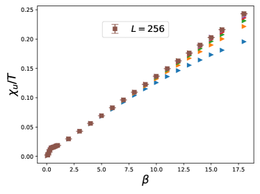
The observable as functions of for = 24, 32, 40,…, 192, 256, and 448 (from top to bottom) for the ladder and the staggered (only up to =256) models are demonstrated in fig. 2. Similarly, fig. 3 contains the results of versus for the honeycomb model.


As can been seen from the top panel of fig. 2 which is associated with the ladder model, although mild (finite) temperature and system size dependence may still be there for the largest lattice, it is clear that the of reaches a (more or less) plateau, i.e., a constant value close to 1.25, for . This is without doubt a character of the quantum critical regime. The horizontal solid line shown in the figure is 1.09 and is the analytic result of this quantity (Ref. Chu94 ). It is obvious that a more detailed theoretical calculation is essential to catch the numerical results obtained here.
The dependence of for the staggered model is demonstrated in the bottom panel of fig. 2. The results in the figure indicate reaches the value of 1 rapidly, both at high and moderate low temperatures. Moreover, no sign of the appearance of a plateau implies the absence of QCR. While further verification is on request, most likely this is a feature of a first order phase transition.
Similar to the outcomes of the ladder model (on the square lattice), the quantity of the honeycomb model reaches a plateau for , see fig. 3.
It is interesting to notice that the results shown in figs. 2 and 3 imply that when compared with the ladder model, larger values of are required for the quantity of the honeycomb model to saturate to its plateau.
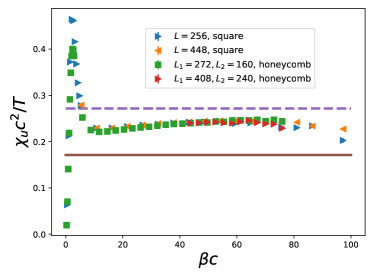
Remarkably, the plateau for both the ladder and the honeycomb models take the same value. In particular, if the data on large lattices of both models are plotted as functions of (The calculations of will be detailed shortly), a good data collapse outcome is obtained, see fig. 4. This indicates it is highly probable that QCR is indeed found in these two models and such an observation in turn provides an evidence for the associated phase transitions to be continuous.

The scenarios reached here are consistent with the known outcomes in the literature regarding the exotic phase transitions of these three investigated models.
III.2
III.2.1 Determination of the spinwave velocity
Since the low-energy constant spinwave velocity is required for calculating the numerical value of , we have determined firstly.
The method used here for the calculations of is the winding numbers squared Kau08 ; Sen15 ; Jia111 ; Jia112 . Specifically, for each considered box size , the is adjusted in the simulations so that three winding numbers squared for and take the same value. When this condition is met, the corresponding to the simulated is .
It should be pointed out that on the honeycomb lattice, square-shape area can only be reached with certain aspect ratios . As a result, the simulations associated with the honeycomb lattice are performed on these aspect ratios (of so the (almost) square-shape area is obtained.
Finally, the calculations are done at = 1.4925, 1.1923, 1.19 for the ladder, the staggered, and the honeycomb models, respectively.
The spatial and the temporal winding numbers squared as functions of for the ladder and the staggered models are shown in the top () and the bottom () panels of fig. 5. In addition, the estimated related to various for the ladder model is demonstrated in fig. 6. A fit of applying the ansatz () to the data of fig. 6 leads to ().


Here we do not conduct the associated fits for the staggered model. This is because as we will show shortly, with the fact that is a constant, the related does not possess the expected feature of QCR. As a result, calculating the bulk for this model is no long needed.
Regarding the of the honeycomb model, the outcome on a lattice of and is quoted here and is given by . We have also carried out simulations on a honeycomb lattice and the resulting is estimated to be . Since is over 0.97 and the ratio of the linear box sizes of these two honeycomb lattices is = 4, one expects negligible finite-lattice effects for the quoted value of .
III.2.2 Determination of
After determining the values of the spinwave velocity for all the three investigated model, we turn to studying the universal quantity .
as a function of for the ladder model is shown in fig. 7. The figure suggests convincingly that the observable of this model reaches a plateau for , which is a feature of QCR. Similar to that of the quantity , this characteristic provides yet another evidence that the corresponding phase transition is likely a second order one. The horizontal solid (2.7185) and dashed (1.7125) lines in fig. 7 represent the theoretical calculations obtained in Refs. Chu94 and Kau08 , respectively. It is clear that the next to leading order large -expansion computations carried out in these references are not sufficient to match the numerical value of determined in this study.
In fig. 8 is considered as a function of for the staggered model. For a first order phase transition, one expects the magnitude of the winding number squared grows with . Hence the rising of in the low temperature region is a signal of first order phase transition for the staggered model. This is consistent with the conclusion established in the literature.
Similar to the outcomes associated with /, the plateaus of for both the ladder and the honeycomb models have the values of about the same magnitude, and a good data collapse result is obtained if the data on large lattices of both models are considered as functions of , again see fig. 9. This observation can also be regarded as an evidence that both the transitions of the ladder and the honeycomb model are likely continuous.
Interestingly, if the data of of both the ladder and the honeycomb models are plotted as functions of , a slightly downgrade quality scaling than that of fig. 9 appears as well.
Finally, it should be pointed out that the trend of moving downward for the quantity at large values of shown in figs. 7 and 9 is due the observable and is an artifact. In particular, to obtain the correct bulk , taking the appropriate order of limits, namely, is essential.

III.3 The spin stiffness
For the ladder model, the quantity as functions of for several are demonstrated in fig. 10. The results in fig. 10 indicate that in the limit , approaches a value between 0.32 and 0.33. This number differ significantly from calculated in Ref. Kau08 . However, if an alternative definition, namely is used, then our calculations lead to in the limit, which is close to the predicted result of .

For the staggered model, it is anticipated that will grow with (in the limit), and this is indeed what’s observed in our data, see fig. 11.

In fig. 12, as functions of is shown for several honeycomb lattices. Although no convergence (as ) is observed, it is interesting to notice that a good data collapse emerges when a logarithmic correction is taken into account. Specifically, if is considered as functions of , then a high quality scaling appears, see fig. 13. This scenario is consistent with that obtained in Ref. Puj13 . Finally, since a free parameter is allowed in the logarithmic correction, namely one can use with being some constant instead of , we do not contrast the results related to the spin stiffness on the honeycomb lattice with that on the square lattice.


IV Discussions and Conclusions
Using the first principle quantum Monte Carlo simulations, we investigate the QCR of three 2D models on both the square and the honeycomb lattices. Particularly, three universal quantities associated with QCR, namely , and are obtained and their () dependence is studied.
Among the three studied models, the ladder and the honeycomb models are shown to possess second order phase transitions from the Néel phase to the VBS phase Lou09 ; Puj13 ; Har13 , and for the staggered model the associated transition is first order Sen10 . Our investigation related to the QCR leads to results consistent with these scenarios.
Specifically, while for the ladder and the honeycomb models, the quantity () of both models reach the same plateau value and a good scaling emerges when considered as a function of , no such behavior is found for the staggered models. Moreover, obtains a constant outcome in the limit for the ladder model. Similar situation applies to the honeycomb model when a logarithmic correction to the observable is taken into account. For the staggered model both the quantities and grow with or . This is in agreement with the fact that the targeted phase transition of the staggered model is first order.
It is surprising to observe that to obtain a good scaling, the universal quantity associated with on the honeycomb lattice requires a logarithmic correction. This is not the case for the same observable on the square lattice. It will be interesting to understand this from a theoretical perspective.
Apart from the three universal quantities considered here, one frequently studied observable associated with QCR is the Wilson ratio . Here is the specific heat and can be calculated directly or through the internal energy density . However, due to the subtlety of both approaches for the determination of shown in Refs. Sen15 ; Pen20 , here we do not attempt to carry out a high precision calculation of the quantity . Nevertheless, the investigation conducted here provide evidence to support the scenario that for the ladder and the honeycomb models, the associated quantum phase transitions from the Néel phase to the VBS phase are likely to be continuous.
The results presented here are not only interesting in themselves, but also can be used as criterions to distinguish second order phase transitions from first order ones for exotic phase transitions such as the DQC studied here.
This study is partially supported by the Ministry of Science and Technology of Taiwan.
References
- (1) Nigel Goldenfeld, Lectures On Phase Transitions And The Renormalization Group (Frontiers in Physics) (Addison-Wesley, 1992).
- (2) J. Cardy, Scaling and Renormalization in Statistical Physics, Cambridge University Press, Cambridge, UK, 1996.
- (3) Lincoln D. Carr, Understanding Quantum Phase Transitions (Condensed Matter Physics) (CRC Press, 2010).
- (4) S. Sachdev, Quantum Phase Transitions (Cambridge University Press, Cambridge, 2nd edition, 2011).
- (5) A. W. Sandvik, Phys. Rev. Lett. 98, 227202 (2007).
- (6) J. Lou, A. W. Sandvik, and N. Kawashima, Phys. Rev. B. 80, 180414(R) (2009).
- (7) Arnab Sen and Anders W. Sandvik Phys. Rev. B 82, 174428 (2010).
- (8) V.L. Ginzburg and L.D. Landau, Zh. Eksp. Teor. Fiz. 20, 1064 (1950). English translation in: L. D. Landau, Collected papers (Oxford: Pergamon Press, 1965) p. 546.
- (9) T. Senthil, L. Balents, S. Sachdev, A. Vishmanath and M. P. A. Fisher, Science 303 1490 (2004).
- (10) T. Senthil, L. Balents, S. Sachdev, A. Vishwanath, and M. P. A. Fisher, Phys. Rev. B 70, 144407 (2004).
- (11) Anatoly Kuklov, Nikolay Prokof’ev, Boris Svistunov, Matthias Troyer, Annals of Physics Volume 321, Issue 7, July 2006, Pages 1602-1621.
- (12) R. G. Melko and R. K. Kaul, Phys. Rev. Lett. 100, 017203 (2008).
- (13) F.-J. Jiang, M. Nyfeler, S. Chandrasekharan, and U.-J. Wiese, J. Stat. Mech. (2008) P02009.
- (14) A. B. Kuklov, M. Matsumoto, N. V. Prokof’ev, B. V. Svistunov, M. Troyer, Phys. Rev. Lett. 101, 050405 (2008).
- (15) A. W. Sandvik, Phys. Rev. Lett. 104, 177201 (2010).
- (16) Kun Chen, Yuan Huang, Youjin Deng, A. B. Kuklov, N. V. Prokof’ev, and B. V. Svistunov Phys. Rev. Lett. 110, 185701 (2013).
- (17) Kenji Harada, Takafumi Suzuki, Tsuyoshi Okubo, Haruhiko Matsuo, Jie Lou, Hiroshi Watanabe, Synge Todo, and Naoki Kawashima Phys. Rev. B 88, 220408(R) (2013).
- (18) Hui Shao, Wenan Guo, Anders W. Sandvik, Science 352, 213 (2016).
- (19) Anders W. Sandvik, Bowen Zhao, Chin. Phys. Lett. 37, 057502 (2020)
- (20) Shumpei Iino, Satoshi Morita, Anders W. Sandvik, Naoki Kawashima, J. Phys. Soc. Jpn. 88, 034006 (2019).
- (21) N. D. Mermin and H. Wagner, Phys. Rev. Lett. 17, 1133 (1966).
- (22) P. C. Hohenberg, Phys. Rev. 158, 383 (1967).
- (23) Sidney Coleman, Communications in Mathematical Physics volume 31, pages 259–264 (1973).
- (24) Axel Gelfert and Wolfgang Nolting, J. Phys.: Condens. Matter 13 R505 (2001).
- (25) A. V. Chubukov and S. Sachdev, Phys. Rev. Lett. 71, 169 (1993).
- (26) A. V. Chubukov and S. Sachdev, Phys. Rev. Lett. 71, 2680 (1993).
- (27) A. V. Chubukov, S. Sachdev, and J. Ye, Phys. Rev. B 49, 11919 (1994).
- (28) A. W. Sandvik, A. V. Chubukov, and S. Sachdev, Phys. Rev. B 51, 16483 (1995)
- (29) M. Troyer, H. Kantani, and K. Ueda, Phys. Rev. Lett. 76, 3822 (1996).
- (30) Matthias Troyer, Masatoshi Imada, and Kazuo Ueda, J. Phys. Soc. Jpn. 66, 2957 (1997).
- (31) Jae-Kwon Kim and Matthias Troyer, Phys. Rev. Lett. 80, 2705 (1998).
- (32) Y. J. Kim, R. J. Birgeneau, M. A. Kastner, Y. S. Lee, Y. Endoh, G. Shirane, and K. Yamada, Phys. Rev. B 60, 3294 (1999).
- (33) Y. J. Kim and R. J. Birgeneau, Phys. Rev. B 62, 6378 (2000).
- (34) A. W. Sandvik, V. N. Kotov, and O. P. Sushkov, Phys. Rev. Lett. 106, 207203 (2011).
- (35) A. Sen, H. Suwa, and A. W. Sandvik, Phys. Rev. B 92, 195145 (2015).
- (36) D.-R. Tan and F.-J. Jiang, Phys. Rev. B 98, 245111 (2018).
- (37) Ribhu K. Kaul, Roger G. Melko, Phys. Rev. B 78, 014417 (2008).
- (38) Ribhu K. Kaul and Subir Sachdev, Phys. Rev. B 77, 155105 (2008).
- (39) Sumiran Pujari, Kedar Damle, and Fabien Alet, Phys. Rev. Lett. 111, 087203 (2013).
- (40) A. W. Sandvik, Phys. Rev. B 55, R14157 (1999).
- (41) A. W. Sandvik, AIP Conf. Proc. 1297, 135 (AIP, New York, 2010).
- (42) F.-J. Jiang, Phys. Rev. B 83, 024419 (2011).
- (43) F.-J. Jiang and U.-J. Wiese, Phys. Rev. B 83, 155120 (2011).
- (44) Jhao-Hong Peng, L.-W. Huang, D.-R. Tan, and F.-J. Jiang, Phys. Rev. B 101, 174404 (2020).