Quantum control via chirped coherent anti-Stokes Raman spectroscopy

Discovery of Raman scattering in the 1920s which coincided with major developments in quantum mechanics, followed by the advancements in laser technology since 1960s paved new ways for understanding the chemical compounds and structure of molecular systems. Modern Raman spectroscopy, that use spontaneous Raman scattering at their core, is characterized by a sufficiently low intensity signal, which is incoherent and isotropic. Being one of the leading non-linear optics techniques, Coherent anti-Stokes Raman Scattering (CARS) spectroscopy makes use of stimulated Raman process resulting in a directional anti-Stokes signal of intensity many orders of magnitude higher than an isotropic spontaneous Raman signal. Because CARS addresses inherent properties of matter, such as vibrational degrees of freedom, it belongs to one of the best suited and most frequently used spectroscopic methods for imaging, sensing and detection without labeling or staining [1, 2, 3, 4, 5]. High sensitivity, high resolution and noninversiveness of CARS have been exploited for imaging of chemical and biological samples [6, 7, 8, 9, 10, 11, 12, 13, 14, 15, 16], standoff detection [17, 18, 20, 19] and combustion thermometry [21, 22]. Recent developments in the applications of CARS in biology include imaging and classification of cancer cells that help early diagnosis [23, 24, 25], and rapid and label-free detection of the SARS-CoV-2 pathogens [26]. CARS has also been used recently for observing real-time vibrations of chemical bonds within molecules [27], direct imaging of molecular symmetry [28], graphene imaging [29], and femtosecond spectroscopy [30, 31].

In this work, we present a theoretical description of a general and robust technique of creating maximal-coherence superpositions of quantum states that can be used to optimize the signals in CARS-based applications.

In the four-wave mixing process of CARS, the pump and Stokes pulses having frequencies $\omega_{p}$ and $\omega_{s}$ respectively excite the molecular vibrations to create a coherent superposition which a probe pulse having frequency $\omega_{pr}$ then interacts with and generate an anti-Stokes signal. The output signal is blue-shifted and has a frequency of $\omega_{as}=\omega_{p}-\omega_{s}+\omega_{pr}$. It is about six orders of magnitude higher in amplitude compared to the spontaneous process and its direction is determined by the phase-matching condition [32, 33, 34, 35]. However, one of the main challenges in CARS has been the presence of non-resonant background appearing in the spectra which limits the image contrast and chemical sensitivity. Another coherent, multi-photon Raman process called Stimulated Raman Scattering (SRS) has an advantage over CARS because of the absence of nonresonant background [36]. In SRS, the frequency difference of pump and Stokes ($\omega_{p}-\omega_{s}$) is matched with the vibrational frequency of the molecule to excite the vibrational transitions. However, the detection of compounds using SRS requires a scheme that is more complicated than CARS as the input and output signals in SRS have the same frequencies. In CARS, the signal can be easily extracted by an optical filter due to the anti-Stokes component having a frequency blue-shifted compared to the incoming pulses [37]. To overcome the limitations of CARS, there has been a tremendous effort applied on removing the background from nonresonant processes and enhancing the signal amplitude [38, 39, 40, 41, 42, 43, 44, 45, 46, 47].

In the framework of Maxwell’s equations, the amplitude of the anti-Stokes field is related to coherence between the electronic vibrational states of the target molecules. Thus, maximizing coherence is the key to optimizing the intensity of anti-Stokes signal [48, 20]. Chirped pulses have been often used in CARS-based imaging techniques to achieve a high spectroscopic resolution [49, 50] and a maximum coherence [51, 52, 53]. A method for selective excitation in a multimode system using a transform-limited pump pulse and a lineraly chirped Stokes pulse in stimulated Raman scattering is proposed in [54]. The effects of chirped pump and Stokes pulses on the nonadiabatic coupling between vibrational modes are discussed in [55]. A ‘roof’ method of chirping to maximize coherence is introduced in [56] based on adiabatic passage in an effective two-level system. In this method, the Stokes pulse is linearly chirped at the same rate as that of the pump pulse during the first half of the pulse duration and is oppositely chirped afterwards.

Here, we discuss a chirping scheme in CARS, in which all the incoming pulses are chirped to achieve the maximum coherence and suppress the background via adiabatic passage. The selectivity, robustness and adiabatic nature of this control scheme make it a viable candidate for improving the current methods for imaging, sensing and detection using CARS.

A schematic diagram of the CARS process is given in Fig. 1. We consider chirped pump, Stokes and probe pulses with temporal chirp rates $\alpha_{q}$, $q=p,s,pr$ as

$$E_{q}(t)=E_{q_{0}}(t)\cos\left[\omega_{q}(t-t_{c})+\frac{\alpha_{q}}{2}(t-t_{c})^{2}\right]$$

(1)

and having Gaussian envelopes

$$E_{q_{0}}(t)=\frac{E_{q0}}{\left(1+\frac{\alpha_{q}^{\prime 2}}{\tau_{0}^{4}}\right)^{1/4}}e^{-\frac{(t-t_{c})^{2}}{2\tau^{2}}},$$

(2)

where $\tau_{0}$ is the transform-limited pulse duration, $\tau$ is the chirp-dependent pulse duration given by $\tau=\tau_{0}[1+\alpha_{q}^{\prime 2}/\tau_{0}^{4}]^{1/2}$ and $\alpha^{\prime}_{q}$ is the spectral chirp rate, which is related to the temporal chirp rate as $\alpha_{q}=\alpha_{q}^{\prime}/\tau_{0}^{2}(1+\alpha_{q}^{\prime 2}/\tau_{0}^{4})$. The interaction Hamiltonian of the four-level system, after defining the one photon detunings, $\Delta_{s}=\omega_{p}-\omega_{31}$ and $\Delta_{as}=\omega_{as}-\omega_{41}$, reads

$$\begin{split}\mathbf{H}_{int}(t)=\frac{\hbar}{2}\left[\Omega_{p}(t)\exp(i\Delta_{s}t-\tfrac{i}{2}\alpha_{p}t^{2})\outerproduct{1}{3}+\right.\\ \left.\Omega_{s}(t)\exp(i\Delta_{s}t-\tfrac{i}{2}\alpha_{s}t^{2})\outerproduct{2}{3}+\right.\\ \left.\Omega_{pr}(t)\exp(i\Delta_{as}t-\tfrac{i}{2}\alpha_{pr}t^{2})\outerproduct{2}{4}+\right.\\ \left.\Omega_{as}(t)\exp(i\Delta_{as}t)\outerproduct{1}{4}+h.c\right]\,,\end{split}$$

(3)

where $\Omega_{q0}=-\mu_{ij}E_{q0}/\hbar$. This Hamiltonian can be simplified to a two-level super-effective Hamiltonian by eliminating states $\ket{3}$ and $\ket{4}$ adiabatically under the assumption of large one-photon detunings. The dynamics of the four-level system interacting with the fields in Eq.(2) is described by the Liouville-von Neumann equation $i\hbar\dot{\bm{\rho}}(t)=[\mathbf{H}_{int}(t),\bm{\rho}(t)].$ We define the two-photon detuning as $\delta=\omega_{p}-\omega_{s}-\omega_{21}=\omega_{as}-\omega_{pr}-\omega_{21}$, make the transformations in the interaction frame $\rho_{11}=\tilde{\rho}_{11}$, $\rho_{12}=\tilde{\rho}_{12}e^{-i(\omega_{1}-\omega_{2})(t-t_{c})}$, $\rho_{13}=\tilde{\rho}_{13}e^{i\omega_{p}(t-t_{c})}$, $\rho_{14}=\tilde{\rho}_{14}e^{i\omega_{as}(t-t_{c})}$, $\rho_{22}=\tilde{\rho}_{22}$, $\rho_{23}=\tilde{\rho}_{23}e^{-i(\omega_{2}-\omega_{1}-\omega_{p})(t-t_{c})}$, $\rho_{24}=\tilde{\rho}_{24}e^{-i(\omega_{2}-\omega_{1}-\omega_{as})(t-t_{c})}$, $\rho_{33}=\tilde{\rho}_{33}$, $\rho_{34}=\tilde{\rho}_{34}e^{-i(\omega_{p}-\omega_{as})(t-t_{c})}$, $\rho_{44}=\tilde{\rho}_{44}$ and obtain a system of differential equations for the density matrix elements

$\displaystyle\begin{aligned} i\dot{\rho}_{11}=&\tfrac{1}{2}\Omega_{p0}(t)e^{\frac{i}{2}\alpha_{p}(t-t_{c})^{2}}\rho_{31}+\tfrac{1}{2}\Omega_{as0}(t)\rho_{41}-c.c\,,\\ i\dot{\rho}_{22}=&\tfrac{1}{2}\Omega_{s0}(t)e^{-i\delta(t-t_{c})+\frac{i}{2}\alpha_{s}(t-t_{c})^{2}}\rho_{32}\\ &+\tfrac{1}{2}\Omega_{pr0}(t)e^{-i\delta(t-t_{c})+\frac{i}{2}\alpha_{pr}(t-t_{c})^{2}}\rho_{42}-c.c\,,\\ i\dot{\rho}_{33}=&\tfrac{1}{2}\Omega^{*}_{p0}(t)e^{-\frac{i}{2}\alpha_{p}(t-t_{c})^{2}}\rho_{13}\\ &+\tfrac{1}{2}\Omega^{*}_{s0}(t)e^{i\delta(t-t_{c})-\frac{i}{2}\alpha_{s}(t-t_{c})^{2}}\rho_{23}-c.c\,,\\ i\dot{\rho}_{44}=&\tfrac{1}{2}\Omega^{*}_{as0}(t)\rho_{14}\\ &+\tfrac{1}{2}\Omega^{*}_{pr0}(t)e^{i\delta(t-t_{c})-\frac{i}{2}\alpha_{s}(t-t_{c})^{2}}\rho_{24}-c.c\,,\\ i\dot{\rho}_{12}=&\tfrac{1}{2}\Omega_{p0}(t)e^{\frac{i}{2}\alpha_{p}(t-t_{c})^{2}}\rho_{32}+\tfrac{1}{2}\Omega_{as0}(t)\rho_{42}\\ &-\tfrac{1}{2}\Omega^{*}_{s0}(t)e^{i\delta(t-t_{c})-\frac{i}{2}\alpha_{s}(t-t_{c})^{2}}\rho_{13}\\ &-\tfrac{1}{2}\Omega^{*}_{pr0}(t)e^{i\delta(t-t_{c})-\frac{i}{2}\alpha_{pr}(t-t_{c})^{2}}\rho_{14}\,,\\ i\dot{\rho}_{13}=&\Delta_{s}\rho_{13}+\tfrac{1}{2}\Omega_{p0}(t)e^{\frac{i}{2}\alpha_{p}(t-t_{c})^{2}}\rho_{33}\\ &+\tfrac{1}{2}\Omega_{as0}(t)\rho_{43}-\tfrac{1}{2}\Omega_{p0}(t)e^{\frac{i}{2}\alpha_{p}(t-t_{c})^{2}}\rho_{11}\\ &-\tfrac{1}{2}\Omega_{s0}(t)e^{-i\delta(t-t_{c})+\frac{i}{2}\alpha_{pr}(t-t_{c})^{2}}\rho_{12}\,,\\ i\dot{\rho}_{14}=&\Delta_{as}\rho_{14}+\tfrac{1}{2}\Omega_{p0}(t)e^{\frac{i}{2}\alpha_{p}(t-t_{c})^{2}}\rho_{34}\\ &+\tfrac{1}{2}\Omega_{as0}(t)\rho_{44}-\tfrac{1}{2}\Omega_{a0}(t)\rho_{11}\\ &-\tfrac{1}{2}\Omega_{pr0}(t)e^{-i\delta(t-t_{c})+\frac{i}{2}\alpha_{pr}(t-t_{c})^{2}}\rho_{12}\,,\\ \end{aligned}$

$\displaystyle\begin{aligned} i\dot{\rho}_{23}=&\Delta_{s}\rho_{23}+\tfrac{1}{2}\Omega_{s0}(t)e^{-i\delta(t-t_{c})+\frac{i}{2}\alpha_{s}(t-t_{c})^{2}}\rho_{33}\\ &+\tfrac{1}{2}\Omega_{pr0}(t)e^{-i\delta(t-t_{c})+\frac{i}{2}\alpha_{pr}(t-t_{c})^{2}}\rho_{43}\\ &-\tfrac{1}{2}\Omega_{p0}(t)e^{\frac{i}{2}\alpha_{p}(t-t_{c})^{2}}\rho_{21}\\ &-\tfrac{1}{2}\Omega_{s0}(t)e^{-i\delta(t-t_{c})-\frac{i}{2}\alpha_{s}(t-t_{c})^{2}}\rho_{22}\,,\\ i\dot{\rho}_{24}=&\Delta_{as}\rho_{24}+\tfrac{1}{2}\Omega_{s0}(t)e^{-i\delta(t-t_{c})+\frac{i}{2}\alpha_{s}(t-t_{c})^{2}}\rho_{34}\\ &+\tfrac{1}{2}\Omega_{pr0}(t)e^{-i\delta(t-t_{c})+\frac{i}{2}\alpha_{pr}(t-t_{c})^{2}}\rho_{44}\\ &-\tfrac{1}{2}\Omega_{as0}(t)\rho_{21}\\ &-\tfrac{1}{2}\Omega_{pr0}(t)e^{-i\delta(t-t_{c})+\frac{i}{2}\alpha_{pr}(t-t_{c})^{2}}\rho_{22}\,,\\ i\dot{\rho}_{34}=&(\Delta_{as}-\Delta_{s})\rho_{34}+\tfrac{1}{2}\Omega^{*}_{p0}(t)e^{-\frac{i}{2}\alpha_{p}(t-t_{c})^{2}}\rho_{14}\\ &+\tfrac{1}{2}\Omega^{*}_{s0}(t)e^{i\delta(t-t_{c})-\frac{i}{2}\alpha_{s}(t-t_{c})^{2}}\rho_{24}\\ &-\tfrac{1}{2}\Omega_{as0}(t)\rho_{31}\\ &-\tfrac{1}{2}\Omega_{pr0}(t)e^{-i\delta(t-t_{c})+\frac{i}{2}\alpha_{pr}(t-t_{c})^{2}}\rho_{32}\,.\\ \end{aligned}$

(4)

As the next step, the condition for chirping of the probe pulse such that $\alpha_{pr}=\alpha_{s}-\alpha_{p}$ is imposed, which is required to equate the exponentials. The above set of equations is then modified by applying the adiabatic elimination, $\dot{\rho}_{33}=\dot{\rho}_{44}=\dot{\rho}_{34}=0$ and substituting for $\rho_{14},\rho_{24},\rho_{23}$ and $\rho_{24}$ in the equations of $\dot{\rho}_{11},\dot{\rho}_{22}$ and $\dot{\rho}_{12}$. After defining the new Rabi frequencies as

$\displaystyle\begin{aligned} \Omega_{1}(t)&=\frac{|\Omega_{p0}(t)|^{2}}{4\Delta_{s}}+\frac{|\Omega_{as0}(t)|^{2}}{4\Delta_{as}}\,,\\ \Omega_{2}(t)&=\frac{|\Omega_{s0}(t)|^{2}}{4\Delta_{s}}+\frac{|\Omega_{pr0}(t)|^{2}}{4\Delta_{as}}\,,\\ \Omega_{3}(t)&=\frac{\Omega_{p0}(t)\Omega^{*}_{s0}(t)}{4\Delta_{s}}+\frac{\Omega^{*}_{pr0}(t)\Omega_{as0}(t)}{4\Delta_{as}}\end{aligned}$

(5)

the density matrix equations are cast into the a set of equations describing the dynamics in the super-effective two-level system

$\displaystyle\begin{aligned} i\dot{\rho}_{11}=&\Omega_{3}(t)e^{i\delta(t-t_{c})-\frac{i}{2}(\alpha_{s}-\alpha_{p})(t-t_{c})^{2}}\rho_{21}-c.c\,,\\ i\dot{\rho}_{22}=&\Omega^{*}_{3}(t)e^{-i\delta(t-t_{c})+\frac{i}{2}(\alpha_{s}-\alpha_{p})(t-t_{c})^{2}}\rho_{12}-c.c\,,\\ i\dot{\rho}_{12}=&\left[\Omega_{1}(t)-\Omega_{2}(t)\right]\rho_{12}\\ &+\Omega_{3}(t)e^{i\delta(t-t_{c})-\frac{i}{2}(\alpha_{s}-\alpha_{p})(t-t_{c})^{2}}(\rho_{22}-\rho_{11})\end{aligned}$

(6)

Further transformations of the density matrix elements such as $\rho_{11}=\tilde{\rho}_{11}$, $\rho_{12}=\tilde{\rho}_{12}e^{i\delta(t-t_{c})-\frac{i}{2}(\alpha_{s}-\alpha_{p})(t-t_{c})^{2}}$, and $\rho_{22}=\tilde{\rho}_{22}$, and shifting the diagonal elements lead to the following super-effective Hamiltonian for the two-level system in the field-interaction representation

$$\small\mathbf{H}_{se}(t)=\frac{\hbar}{2}\left(\begin{array}[]{cc}\delta-(\alpha_{s}-\alpha_{p})(t-t_{c})+\Omega_{1}(t)-\Omega_{2}(t)&2\Omega_{3}(t)\\ 2\Omega^{*}_{3}(t)&-\delta+(\alpha_{s}-\alpha_{p})(t-t_{c})-\Omega_{1}(t)+\Omega_{2}(t)\\ \end{array}\right)\,.$$

(7)

The amplitudes of incoming fields are manipulated to make the AC Stark shifts equal, $\Omega_{1}(t)=\Omega_{2}(t)$, and cancel out. This condition is satisfied by taking $\Omega_{s0}=\Omega_{pr0}=\Omega_{p0}/\sqrt{2}$, considering the fact that the anti-Stokes signal is absent in the beginning of the process, $\Omega_{as0}=0$. The effective Rabi frequency $\Omega_{3}(t)$ reads

$$\Omega_{3}(t)=\frac{\Omega_{3(0)}}{\left[(1+\frac{\alpha_{p}^{\prime 2}}{\tau_{0}^{4}})(1+\frac{\alpha_{s}^{\prime 2}}{\tau_{0}^{4}})\right]^{1/4}}e^{-\frac{(t-t_{c})^{2}}{\tau^{2}}}\,.$$

(8)

The peak effective Rabi frequency of transform-limited pulses $\Omega_{3(0)}$ is given by $\Omega_{3(0)}=\Omega_{p0}^{2}/(4\sqrt{2}\Delta)$. It is reduced when chirping is applied to the pump and Stokes pulses with the spectral rates $\alpha_{p}^{\prime}$ and $\alpha_{s}^{\prime}$ respectively. The relative amplitudes of all the Rabi frequencies involved in the dynamics of are shown in Fig. 2. In this paper, all the frequency parameters are defined in the units of the frequency $\omega_{21}$ and time parameters are defined in the units of $\omega^{-1}_{21}$.

During the interaction, at time $t=t_{c}+\delta/(\alpha_{s}-\alpha_{p})$, the diagonal elements become equal to zero creating a coherent superposition state having equal populations of states $\ket{1}$ and $|\ket{2}$ and, therefore, a maximum value of coherence $\rho_{21}$. This time can be determined for a fixed value of two-photon detuning, $\delta$. At the two-photon resonance, the system reaches this maximum coherence at the central time $t_{c}$. It is further preserved in the state of the maximum coherence by imposing the condition of $(\alpha_{s}-\alpha_{p})=0$ in the second half of the pulse duration. A smooth realization of this scheme is possible by choosing the temporal chirp rates of the pump and Stokes pulses to be the same in magnitude and opposite in sign before the central time and equal in sign after that, along with the condition imposed for the chirp rate of probe pulse such that $\alpha_{pr}=\alpha_{s}-\alpha_{p}$, which was deduced to arrive into the Hamiltonian in Eq. (7). This chirping scheme, namely C-CARS, is summarized as follows: $\alpha_{p}=-\alpha_{s}$ and $\alpha_{pr}=2\alpha_{s}$ for $t\leq t_{c}$, and $\alpha_{p}=\alpha_{s}$ and $\alpha_{pr}=0$ for $t>t_{c}$. The Wigner-Ville distributions of the incident pulses are found to be

$$\begin{split}W_{E_{q}}(t,\omega)=\frac{\tau\sqrt{\pi}}{2}E_{q_{0}}e^{-(t-t_{c})^{2}/\tau^{2}}\left[e^{-\tau^{2}[\omega-\omega_{q}-\alpha_{q}(t-t_{c})]^{2}}\right.\\ \left.+e^{-\tau^{2}[\omega+\omega_{q}+\alpha_{q}(t-t_{c})]^{2}}\right].\end{split}$$

(9)

The positive solutions of these equations are depicted in Fig. 3. The “turning off” of chirping in the second half of the pulse duration is the essence of this scheme, resulting in a selective excitation of the molecules and suppressing any off-resonant background. If $\alpha_{p}$ is not reversed, the coherence is not preserved leading to population inversion between states $\ket{1}$ and $\ket{2}$.

To demonstrate the selective excitation of molecules using C-CARS, the time evolution of populations $\rho_{11}$ and $\rho_{22}$ and coherence $\rho_{12}$ is presented in Fig. 4 for four different cases described below. The C-CARS control scheme is applied for the resonant ($\delta=0$) and off-resonant ($\delta\neq 0$) case respectively in figures 4(a) and 4(b). The coherence reaches maximum at the central time in the resonant case, and is preserved till the end of dynamics owing to the zero net chirp rate attained by reversing the sign of $\alpha_{p}$. On the contrary, the time of the maximum coherence does not coincide with the central time in the non-resonant case, which results in a population transfer to the upper state and zero coherence. To emphasize the significance of reversing the sign of $\alpha_{p}$ in C-CARS control scheme we compare it with the scheme when the pump and Stokes are oppositely chirped for the whole pulse duration, $\alpha_{p}=-\alpha_{s}$. For this case the dynamics of the system is plotted in figures 4(c) and 4(d) for $\delta=0$ and $\delta=0.1$ respectively. In (c), even though the system reaches a perfect coherence at $t=t_{c}$, it drops to zero because population is further adiabatically transferred to state $|2\rangle$. Coherence in (d) behaves similar to that of (b).

The validity of adiabatic approximation, which led to a derivation of the super-effective Hamiltonian, can be tested by comparing the results of the super-effective two-level system with the exact solution using the Liouville von Neumann equation for the four-level system. To this end, the condition for chirping of the probe pulse $\alpha_{pr}=\alpha_{s}-\alpha_{p}$ is applied to the field-interaction Hamiltonian of the four level system

$$\begin{split}&\mathbf{H}_{ex}(t)\\ =&\frac{\hbar}{2}\begin{pmatrix}2\alpha_{p}(t-t_{c})&0&\Omega_{p_{0}}(t)&\Omega_{as_{0}}(t)\\ 0&2[\alpha_{s}(t-t_{c})-\delta]&\Omega_{s_{0}}(t)&\Omega_{pr_{0}}(t)\\ \Omega_{p_{0}}(t)&\Omega_{s_{0}}(t)&-2\Delta_{s}&0\\ \Omega_{as_{0}}(t)&\Omega_{pr_{0}}(t)&0&2[\alpha_{p}(t-t_{c})-\Delta_{as}]\end{pmatrix}\end{split}$$

(10)

Figure 5 shows the contour-plot of vibrational coherence $\rho_{12}$ at the end of dynamics as a function of the peak Rabi frequency $\Omega_{3(0)}(t)$ and dimensionless spectral chirp rate $\alpha_{s}^{\prime}/\tau_{0}^{2}$. Figures (a) and (b) represent the $\delta=0$ and $\delta=0.1$ cases, respectively, of the super-effective two level system, and (c) and (d) represent the same cases obtained by the exact solution of the four-level system using the same set of parameters. In all the figures, the one-photon detuning is $\Delta_{s}=\Delta_{as}=\Delta=1.0$. Around the region where $\alpha_{s}^{{}^{\prime}}/\tau_{0}^{2}=0$, adiabatic passage breaks down and the approximate solution disagrees with the exact solution. As the magnitude of spectral chirp rate increases, the adiabatic approximation coincides with the exact one because the Landau– Zener parameter is well in the adiabatic range, $\Omega_{3(0)}^{2}/|\alpha_{p}|\gg 1$. In the resonant cases (a) and (c), the coherence is at the maximum, (blue color), for the most part, indicating the robustness of C-CARS chirping scheme in preparing the system in a coherent superposition. In the off-resonant case, zero coherence, (red color), is observed for the most part, which is in a stark contrast with the resonant case, revealing the selective nature of coherent excitation using the C-CARS control scheme.

When the electromagnetic field interacts with any quantum system, the eigenstates undergo a rearrangement resulting in a set of quantum states that are said to be ‘dressed’ by the light. These states are called dressed states and the initial states that were ‘untouched’ by the light are called bare states [57]. The robustness of the C-CARS control scheme stems from the adiabatic nature of the light-matter interaction, which can be demonstrated by analyzing the evolution of dressed state energies in the super-effective two-level system. To this end, the density matrix $\bm{\rho}(t)$ is transformed to a dressed density matrix using the transformation $\bm{\rho}_{d}(t)=\mathbf{T}(t)\bm{\rho}(t)\mathbf{T}^{\dagger}(t),$ where $\mathbf{T}(t)$ is an orthogonal matrix given by:

$$\mathbf{T}(t)=\begin{pmatrix}\cos\theta(t)&-\sin\theta(t)\\ \sin\theta(t)&\cos\theta(t)\\ \end{pmatrix}\,.$$

(11)

The Liouville-von Neumann equation for the dressed density matrix is derived from the bare state density matrix equation and reads

	$\displaystyle i\hbar\derivative{t}\bm{\rho}(t)$	$\displaystyle=$	$\displaystyle i\hbar\derivative{t}\left(\mathbf{T}^{\dagger}(t)\bm{\rho}_{d}(t)\mathbf{T}(t)\right)$		(12)
		$\displaystyle=$	$\displaystyle\left[\mathbf{H}_{se}(t),\,\mathbf{T}^{\dagger}(t)\bm{\rho}_{d}(t)\mathbf{T}(t)\right]\,.$

After expanding this equation and using $\dot{\mathbf{T}}(t)\mathbf{T^{\dagger}}(t)=-\mathbf{T}(t)\dot{\mathbf{T}}^{\dagger}(t)\,,$ we arrive at

	$\displaystyle i\hbar\dot{\bm{\rho}}_{d}(t)$	$\displaystyle=$	$\displaystyle\left[\mathbf{T}(t)\mathbf{H}_{se}(t)\mathbf{T^{\dagger}}(t)-i\hbar\mathbf{T}(t)\dot{\mathbf{T}}^{\dagger}(t),\,\bm{\rho}_{d}(t)\right]$		(13)
		$\displaystyle=$	$\displaystyle\left[\mathbf{H}_{d}(t),\,\bm{\rho}_{d}(t)\right]\,,$

where $\mathbf{T}(t)\mathbf{H}_{se}(t)\mathbf{T^{\dagger}}(t)$ is a diagonal matrix. For adiabatic passage to occur, the dressed state Hamiltonian $\mathbf{H}_{d}(t)$ should give the dressed state energies separation greater than $\mathbf{T}(t)\mathbf{\dot{T}^{\dagger}}(t)$ to avoid coupling between dressed states [57, 58, 59]. The dressed state Hamiltonian is found to be

$$\mathbf{H}_{d}(t)=\frac{\hbar}{2}\begin{pmatrix}-\sqrt{(-\delta+\alpha_{pr}(t-t_{c}))^{2}+(2\Omega_{3}(t))^{2}}&-i\dot{\theta}(t)\\ i\dot{\theta}(t)&\sqrt{(-\delta+\alpha_{pr}(t-t_{c}))^{2}+(2\Omega_{3}(t))^{2}}\\ \end{pmatrix}\,,$$

(14)

where the non-adiabatic parameter $\dot{\theta}(t)$, which comes from the matrix $\mathbf{T}(t)\mathbf{\dot{T}^{\dagger}}(t)$, is given by

$\displaystyle\dot{\theta}(t)$

$\displaystyle=\frac{(-\delta+\alpha_{pr}(t-t_{c}))\dot{\Omega}_{3}(t)-2\Omega_{3}(t)\alpha_{pr}}{(-\delta+\alpha_{pr}(t-t_{c}))^{2}+4\Omega_{3}(t)^{2}}\,.$

(15)

Analyzing the equation for $\dot{\theta}(t)$ reveals the selective nature of adiabatic passage in the case of resonance. In the resonant case, the C-CARS chirping scheme ensures that the process be adiabatic in the second half of the pulse by keeping the non-adiabatic coupling parameter $\dot{\theta}(t)$ at zero during this time period. But adiabaticity is not guaranteed in the off-resonant case due to the non-zero factor $\delta$ in the equation. This is demonstrated in Fig.  6, where the bare state energies are given by $E_{1}(t)={H}_{se_{11}}(t)$ and $E_{2}(t)={H}_{se_{22}}(t)$ and the dressed state energies are given by $\lambda_{1}(t)={H}_{d_{11}}(t)$ and $\lambda_{2}(t)={H}_{d_{22}}(t)$. The figures (a) and (b) represent resonant ($\delta=0$) and off-resonant ($\delta\neq 0$) cases when C-CARS control scheme is used. Clearly, the $\dot{\theta}(t)$, dark sold line, has non-zero values in the second half when the system is detuned. The perfectly adiabatic nature of interaction in Fig. 6(a) corresponds to the maximum coherence in Fig. 4(a) and the non-adiabatic nature in Fig. 6(b) corresponds to the population inversion in Fig. 4(b). The parameters used in Fig. 6 are the same as that used in Fig. 4. In figures 6(c) and 6(d), the same quantities are plotted for $\delta=0$ and $\delta\neq 0$ respectively for the scheme when the pump and Stokes are chirped oppositely for the whole pulse duration. The process is perfectly adiabatic only in the second half of (a) since a smooth realization of $\dot{\theta}(t)=0$ was made possible owing to the developed C-CARS control scheme. The dynamics is much different and the selective excitation does not happen when the effective Rabi frequency, $\Omega_{3}(t)$, is not strong enough as shown in Fig. 7 where $\Omega_{3}(0)=0.18$, $\alpha_{s}^{\prime}/\tau_{0}^{2}=-0.8$ and $\tau_{0}=25[\omega^{-1}_{21}]$. In both (a), $\delta=0$ and (b), $\delta=0.1$ cases, the non-adiabatic coupling parameter is much greater compared to Fig. 6. In the off-resonant case (d), the coherence oscillates much stronger compared to the resonant case (c) showing the absence of adiabatic passage.

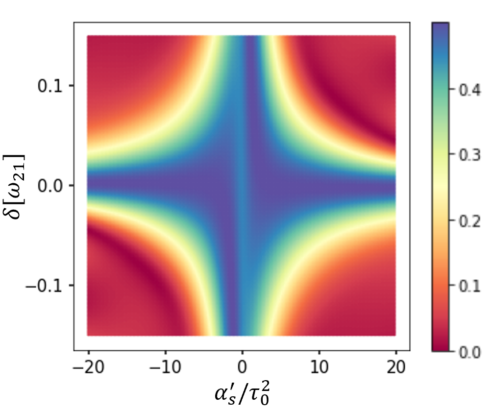
To investigate how the value of two-photon detuning and spectral chirp rate are related to the selectivity in C-CARS method, the end-of-pulse vibrational coherence is plotted as a function of $\delta$ and $\alpha_{s}^{\prime}/\tau_{0}^{2}$ in Fig. 8. At the two-photon resonance, coherence is at the maximum for all the values of chirp rate. If the detuning is large, a small chirp rate can selectively excite the system while for smaller values of detuning, the chirp rate needs to be increased in order to suppress excitation of close vibrational frequencies and the non-resonant background. This provides a way to control the selectivity by adjusting the values of chirp rate. The plot is symmetric across the diagonal lines as flipping the signs of both $\alpha_{s}$ and $\delta$ will not change the dynamics; it would only result in switching of the diagonal elements in Hamiltonian (7). The plot is also nearly symmetric across the $\delta=0$ line, indicating that the selectivity holds for both red and blue detunings. When the chirp rate is close to zero, the pulses are transform-limited, implying that the maximum coherence and selectivity provided by the chirping scheme is absent in this region. This explains the vertical line present at the 0 of abscissa.

In summary, we presented a control scheme to prepare the ground electronic-vibrational states in the four-level system of CARS in a maximally coherent superposition. We derived the Hamiltonian for a ‘super-effective’ two-level system employing the adiabatic approximation. This two-level Hamiltonian is used to derive the conditions for adiabatic passage necessary for the implementation of the selective excitation of spectrally close vibrations. The amplitudes of the Stokes and probe pulses have to be equal and should be $\sqrt{2}$ times that of the pump pulse. The pump pulse should be chirped at the same rate as the Stokes pulse before the central time and at opposite rate after that. The probe pulse has to be chirped at a rate equal the difference between the chirp rates of the Stokes and the pump pulses for the whole pulse duration. The solutions of Liouville-von Neumann equation show that vibrational coherence is preserved until the end of dynamics in the resonant case due to the adiabatic nature of the interaction. At two-photon resonance, vibrational coherence is maximum, 0.5, for a wide range of field parameters revealing the robustness of the method. Conversely, coherence is almost zero in the off-resonant case for most of the peak Rabi frequency values and the chirp parameters. A comparison of coherence in the four-level and the two-level systems reveals that the adiabatic approximation is valid except when the chirp rate is almost equal to zero. A dressed-state analysis reveals the details of the mechanism of adiabatic passage using C-CARS control scheme.

The presented C-CARS method can find important applications in sensing and imaging of molecular species because it creates a maximally coherent superposition of vibrational states in coherent anti-Stokes Raman scattering allowing the system to emit an optimized signal suitable for detection. The robustness of this method against changes in Rabi frequencies and chirp rates is helpful in experiments. The method helps suppress the background species and excite only the desired ones; the resolution needed for this distinction can be controlled by the chirp parameter.

References

- [1] Cheng J X and Xie X S 2013 Coherent Raman Scattering Microscopy, Taylor & Francis Group, LLC
- [2] Evans, C L and Xie, X S 2008 Coherent Anti-Stokes Raman Scattering Microscopy: Chemical Imaging for Biology and Medicine. Annual Review of Analytical Chemistry 1 883–909.
- [3] Cheng J X and Xie X S 2004 Coherent Anti-Stokes Raman Scattering Microscopy: Instrumentation, Theory, and Applications. J. Phys. Chem. B 108 827-840
- [4] Day J P, Domke K F, Rago G, Kano H, Hamaguchi H-o, Vartiainen E M and Bonn M 2011 Quantitative coherent anti-stokes raman scattering (CARS) microscopy J. Phys. Chem. B 115 7713–25
- [5] Xu S, Camp C H, Lee Y J 2022 Coherent anti-Stokes Raman scattering microscopy for polymers. J. Polym. Sci 60 1244-65.
- [6] Zumbusch A, Holtom G R and Xie X S 1999 Three-Dimensional Vibrational Imaging by Coherent Anti-Stokes Raman Scattering Phys. Rev. Lett. 82, 4142–4145
- [7] Evans C L, Potma E O, Puoris’haag M, Côté D, Lin C P and Xie X S 2005 Chemical imaging of tissue in vivo with video-rate coherent anti-stokes raman scattering microscopy Proceedings of the National Academy of Sciences 102 16807–12
- [8] Cheng J-X, Jia Y K, Zheng G and Xie X S 2002 Laser-scanning coherent anti-stokes raman scattering microscopy and applications to Cell Biology Biophysical Journal 83 502–9
- [9] Volkmer A, Cheng J-X and Sunney Xie X 2001 Vibrational imaging with high sensitivity via epidetected coherent Anti-Stokes Raman scattering microscopy Phys. Rev. Lett. 87 023901
- [10] Potma E O, de Boeij W P, van Haastert P J and Wiersma D A 2001 Real-time visualization of intracellular hydrodynamics in single living cells Proceedings of the National Academy of Sciences 98 1577–82
- [11] Nan X, Potma E O and Xie X S 2006 Nonperturbative chemical imaging of organelle transport in living cells with coherent anti-stokes raman scattering microscopy Biophysical Journal 91 728–35
- [12] Potma E O and Xie X S 2003 Detection of single lipid bilayers with coherent anti-stokes raman scattering (CARS) microscopy Journal of Raman Spectroscopy bf 34 642–50
- [13] Potma E O, Xie X S, Muntean L, Preusser J, Jones D, Ye J, Leone S R, Hinsberg W D and Schade W 2003 Chemical imaging of photoresists with coherent anti-stokes raman scattering (CARS) microscopy J. Phys. Chem. B 108 1296–301
- [14] Balu M, Liu G, Chen Z, Tromberg B J and Potma E O 2010 Fiber delivered probe for efficient cars imaging of tissues Optics Express 18 2380
- [15] Schaller R D, Ziegelbauer J, Lee L F, Haber L H and Saykally R J 2002 Chemically selective imaging of subcellular structure in human hepatocytes with coherent Anti-Stokes Raman scattering (CARS) near-field scanning optical microscopy (NSOM) J. Phys. Chem. B 106 8489–92
- [16] Camp Jr C H, Lee Y J, Heddleston J M, Hartshorn C M, Walker A R, Rich J N, Lathia J D and Cicerone M T 2014 High-speed coherent Raman fingerprint imaging of biological tissues Nature Photonics 8 627–34
- [17] Li H, Harris D A, Xu B, Wrzesinski P J, Lozovoy V V and Dantus M 2008 Coherent mode-selective Raman excitation towards standoff detection Optics Express 16 5499
- [18] Bremer M T and Dantus M 2013 Standoff explosives trace detection and imaging by selective stimulated Raman scattering Applied Physics Letters 103 061119
- [19] Petrov G I, Yakovlev V V, Sokolov A V and Scully M O 2005 Detection of bacillus subtilis spores in water by means of broadband coherent anti-stokes raman spectroscopy Optics Express 13 9537
- [20] Ooi C H, Beadie G, Kattawar G W, Reintjes J F, Rostovtsev Y, Zubairy M S and Scully M O 2005 Theory of femtosecond coherent anti-stokes raman backscattering enhanced by quantum coherence for standoff detection of bacterial spores Phys. Rev. A 72 023807
- [21] Roy S, Gord J R and Patnaik A K 2010 Recent advances in coherent anti-stokes raman scattering spectroscopy: Fundamental developments and applications in reacting flows Progress in Energy and Combustion Science 36 280–306
- [22] Richardson D R, Stauffer H U, Roy S and Gord J R 2017 Comparison of chirped-probe-pulse and hybrid femtosecond/picosecond coherent anti-stokes raman scattering for combustion thermometry Applied Optics 56
- [23] Petrov G I, Arora R and Yakovlev V V 2021 Coherent anti-stokes raman scattering imaging of microcalcifications associated with breast cancer The Analyst 146 1253–9
- [24] Aljakouch K, Hilal Z, Daho I, Schuler M, Krauß S D, Yosef H K, Dierks J, Mosig A, Gerwert K and El-Mashtoly S F 2019 Fast and noninvasive diagnosis of cervical cancer by coherent anti-stokes raman scattering Analytical Chemistry 91 13900–6
- [25] Legesse F B, Medyukhina A, Heuke S and Popp J 2015 Texture analysis and classification in coherent anti-stokes raman scattering (CARS) microscopy images for automated detection of skin cancer Computerized Medical Imaging and Graphics 43 36–43
- [26] Tabish T A, Narayan R J and Edirisinghe M 2020 Rapid and label-free detection of covid-19 using coherent anti-stokes raman scattering microscopy MRS Communications 10 566–72
- [27] Yampolsky S, Fishman D A, Dey S, Hulkko E, Banik M, Potma E O and Apkarian V A 2014 Seeing a single molecule vibrate through time-resolved coherent anti-stokes raman scattering Nature Photonics 8 650–6
- [28] Cleff C, Gasecka A, Ferrand P, Rigneault H, Brasselet S and Duboisset J 2016 Direct imaging of molecular symmetry by coherent anti-stokes Raman scattering Nature Communications 7
- [29] Virga A, Ferrante C, Batignani G, De Fazio D, Nunn A D, Ferrari A C, Cerullo G and Scopigno T 2019 Coherent anti-stokes raman spectroscopy of single and multi-layer graphene Nature Communications 10
- [30] Bohlin A and Kliewer C J 2014 Two-beam ultrabroadband coherent anti-stokes raman spectroscopy for high resolution gas-phase multiplex imaging Applied Physics Letters 104 031107
- [31] Bohlin A, Mann M, Patterson B D, Dreizler A and Kliewer C J 2015 Development of two-beam femtosecond/picosecond one-dimensional rotational coherent anti-stokes raman spectroscopy: Time-resolved probing of flame wall interactions Proceedings of the Combustion Institute 35 3723–30
- [32] Moura C C, Tare R S, Oreffo R O and Mahajan S 2016 Raman spectroscopy and coherent anti-stokes raman scattering imaging: Prospective tools for monitoring skeletal cells and skeletal regeneration Journal of The Royal Society Interface 13 20160182
- [33] Zheltikov A M 2000 Coherent anti-stokes raman scattering: From proof-of-the-principle experiments to femtosecond cars and higher order wave-mixing generalizations Journal of Raman Spectroscopy 31 653–67
- [34] Romanov D, Filin A, Compton R and Levis R 2007 Phase matching in femtosecond boxcars Optics Letters 32 3161
- [35] Pestov D, Ariunbold G O, Murawski R K, Sautenkov V A, Sokolov A V, and Scully M O 2007 Coherent versus incoherent Raman scattering: molecular coherence excitation and measurement, Opt. Lett. 32, 1725
- [36] Freudiger C W, Min W, Saar B G, Lu S, Holtom G R, He C, Tsai J C, Kang J X and Xie X S 2008 Label-free biomedical imaging with high sensitivity by stimulated Raman scattering microscopy Science 322 1857–61
- [37] Krafft C, Dietzek B, Schmitt M and Popp, J 2012 Raman and Coherent Anti-Stokes Raman Scattering Microspectroscopy for Biomedical Applications. Journal of Biomedical Optics, 17 040801.
- [38] Potma E O, Evans C L and Xie X S 2006 Heterodyne coherent anti-stokes raman scattering (CARS) imaging Optics Letters 31 241
- [39] Evans C L, Potma E O and Xie X S 2004 Coherent anti-Stokes Raman scattering spectral interferometry: determination of the real and imaginary components of nonlinear susceptibility for vibrational microscopy Optics Letters 29 2923
- [40] Oron D, Dudovich N and Silberberg Y 2003 Femtosecond phase-and-polarization control for background-free coherent anti-stokes raman spectroscopy Physical Review Letters 90 213902
- [41] Gachet D, Billard F and Rigneault H 2008 Focused field symmetries for background-free coherent anti-stokes Raman spectroscopy Phys. Rev. A 77 061802
- [42] Selm R, Winterhalder M, Zumbusch A, Krauss G, Hanke T, Sell A and Leitenstorfer A 2010 Ultrabroadband background-free coherent anti-stokes raman scattering microscopy based on a compact ER:Fiber Laser System Optics Letters 35 3282
- [43] Konorov S O, Blades M W and Turner R F 2010 Lorentzian amplitude and phase pulse shaping for nonresonant background suppression and enhanced spectral resolution in coherent Anti-Stokes Raman scattering spectroscopy and microscopy Applied Spectroscopy 64 767–74
- [44] Lombardini A, Mytskaniuk V, Sivankutty S, Andresen E R, Chen X, Wenger J, Fabert M, Joly N, Louradour F, Kudlinski A and Rigneault H 2018 High-resolution multimodal flexible coherent Raman endoscope Light, Science & Applications 7
- [45] Richardson D R, Lucht R P, Kulatilaka W D, Roy S and Gord J R 2011 Theoretical modeling of single-laser-shot, chirped-probe-pulse femtosecond coherent anti-stokes raman scattering thermometry Appl. Phys. B 104 699–714
- [46] Pestov D, Murawski R K, Ariunbold G O, Wang X, Zhi M, Sokolov A V, Sautenkov V A, Rostovtsev Y V, Dogariu A, Huang Y and Scully M O 2007 Optimizing the laser-pulse configuration for coherent Raman spectroscopy Science 316 265–8
- [47] Kumar V, Osellame R, Ramponi R, Cerullo G and Marangoni M 2011 Background-free broadband CARS spectroscopy from a 1-MHz ytterbium laser Optics Express 19 15143
- [48] Chathanathil J, Liu G and Malinovskaya S A 2021 Semiclassical control theory of coherent anti-stokes raman scattering maximizing vibrational coherence for remote detection Phys. Rev. A 104 043701
- [49] Knutsen K P, Messer B M, Onorato R M and Saykally R J 2006 Chirped coherent anti-stokes raman scattering for high spectral resolution spectroscopy and chemically selective imaging J. Phys. Chem. B 110 5854–64
- [50] Onorato R M, Muraki N, Knutsen K P and Saykally R J 2007 Chirped coherent anti-stokes raman scattering as a high-spectral- and spatial-resolution microscopy Optics Letters 32 2858
- [51] Pandya N, Liu G, Narducci F A, Chathanathil J and Malinovskaya S 2020 Creation of the maximum coherence via adiabatic passage in the four-wave mixing process of coherent anti-stokes raman scattering Chem. Phys. Lett. 738 136763
- [52] Malinovsky V S 2009 Creating maximum coherence using chirped pulses without adiabatic elimination of excited states Journal of Raman Spectroscopy 40 817–21
- [53] Malinovskaya S A 2007 Chirped Pulse Control Methods for Imaging of Biological Structure and Dynamics Int. J. Quant. Chem. 107 3151
- [54] Malinovskaya S A 2006 Mode-selective excitation using ultrafast chirped laser pulses Phys. Rev. A 73
- [55] Patel V and Malinovskaya S A 2011 Nonadiabatic effects induced by the coupling between vibrational modes via Raman fields Phys. Rev. A 83
- [56] Malinovskaya S A and Malinovsky V S 2007 Chirped-pulse adiabatic control in co- herent anti-Stokes Raman scattering for imaging of biological structure and dynamics Optics Letters 32 707
- [57] Berman P R and Salomaa R 1982 Comparison between dressed-atom and bare-atom pictures in laser spectroscopy Phys. Rev. A 25 2667–92
- [58] Kuklinski J R, Gaubatz U, Hioe F T and Bergmann K 1989 Adiabatic population transfer in a three-level system driven by delayed laser pulses Phys. Rev. A 40 6741–4
- [59] Bergmann K, Vitanov N V and Shore B W 2015 Perspective: Stimulated raman adiabatic passage: The status after 25 Years The Journal of Chemical Physics 142 170901