Quantum BPS Cosmology
Abstract
There has been much discussion about the initial conditions
of the early Universe in the context of quantum theory. In this paper, we
construct the wave function and probability distribution by adopting the quantum
version of the BPS equation instead of the usual Wheeler–DeWitt equation in a
minisuperspace quantum cosmology with spatially uniform scalar fields. Although
the model treated in this study is technically valid for a limited form of scalar
potential, we show that it is possible to construct a conserved probability
current in our model. We also examine classical and quantum aspects of models
with the Dirac–Born–Infeld type scalar fields.
Keywords:
Quantum cosmology, BPS equation, DBI theory
I Introduction
Quantum cosmology Halliwell ; Kiefer0 ; Kiefer1 in minisuperspace is based on the idea that the Hamiltonian constraint in a gravitating system containing a finite number of variables, such as scale factors and scalar fields, is interpreted as a differential equation of the wave function of the Universe. This equation, the Wheeler–DeWitt equation for a minisuperspace, becomes a hyperbolic second-order partial differential equation by a straightforward construction. This makes it difficult to define a positive-definite probability density. Various solutions have been proposed for this problem in definition of the probability density, including a simple and conventional adoption of the square of the absolute value of the wave function. Furthermore, determining what kind of “initial conditions” to solve the Wheeler–DeWitt equation is the most important when considering the very early universe. For this purpose, we have only to choose plausible initial conditions to solve the equation.222Note that it is known that the wave packet solution obtained by the conventional method and interpretation corresponds to the classical solution in the gravitational system KN ; Kiefer2 ; Kiefer3 ; GS ; KKST2 .
Recently, Russo Russo2 ; Russo1 has been studying a class of Einstein gravity theories involving scalar fields in which the classical equations of motion are reduced to first-order ordinary differential equations of time, such as the BPS equations.333The same or similar systems have been considered by many authors SB ; BGLM ; BLRR ; SA ; Lidsey ; Taylor from the past to the present, but there has been little mutual citation between them. The first-order differential equation represents the streamline in phase space, and has the advantage that the behavior of the dynamical system can be directly obtained. Although solvable systems are special cases, they often play an important role in the development of all areas of physics. The solutions of BPS type equations may not, of course, represent all possible solutions of the original equations of motion. Solution with restrictions become effective only when the existence of underlying symmetries, such as supersymmetry (or mock symmetry), is presumed. It seems that the model including scalars discussed here includes the possibility of being connected to fundamental theories with supersymmetry such as string theory. Quantum cosmology with supersymmetry has already been actively researched Graham1 ; Graham2 ; OSB ; OPR ; RB ; Moniz , but in this paper we will be careful to analyze the model without specifying the symmetry.
On the other hand, a quantum version of the BPS equation has already been used through studies of partition functions in topological string theory OVV ; CV . Therefore, we will use the quantum version of the BPS equation as an alternative version of the Wheeler–DeWitt equation for the similar model to Russo’s model, and study the solution to the wave function of the Universe obtained from the equation. This could provide a new perspective on plausible choice of initial conditions for restricted wave functions of the Universe. Our goal is to learn something useful about the probability interpretation of such solutions.
Therefore, although the origins of symmetries and restrictions are not discussed in the current simple models, as mentioned earlier, we must choose a solution that is compatible with the appropriate initial conditions of the quantum Universe. We believe that there is some significance in examining whether the wave function of the specious Universe can be obtained from the BPS-like equation.
The structure of this paper is as follows. Section II reviews Russo’s work on classical cosmological equations. In Section III, we consider the BPS-like equations and their quantum version, and find the specific solution of the wave function. The construction of probability density will be discussed in Section IV. In Section V, we examine cosmology of the Dirac–Born–Infeld type model by use of the BPS equation for the model. The final section provides a summary and future prospects.
We use metric signature and units . are coordinate indices of spacetime, while are indices for space.
II Review of classical cosmology with multiscalar fields
In this section, we briefly review Russo’s model Russo2 ; Russo1 in -dimensional spacetime. The action describing the system of gravitating scalar fields is as follows:
| (1) |
where denotes the determinant of the metric tensor , is the inverse of the metric tensor, is the scalar curvature, are the scalar fields, and is the potential of scalar fields . The metric of the internal space is given by a symmetric matrix, and is generally dependent on scalar fields . Further, the metric of the dimensional spacetime is assumed as
| (2) |
where is a constant, and
| (3) |
and is a scale factor of the flat, homogeneous and isotropic space. Note that this metric becomes the standard Friedmann–Lemaître–Robertson–Walker metric when , while the metric becomes a conformally-flat metric when .
Assuming that all scalar fields are also spatially uniform, that is, a function of time only, , the effective Lagrangian on these variables is given by444The Gibbons–Hawking–York term York ; GH is implicitly taken into account, as a standard approach in Einstein gravity.
| (4) |
where and the dot denotes the time derivative.
These equations are satisfied by the following two simultaneous equations including the first-order derivative:
| (7) |
where the constant satisfies , , and is the inverse matrix of , if the scalar potential takes the following form:
| (8) | |||||
where
| (9) |
and
| (10) |
The potential is mostly determined by , so we call prepotential.
We find that the Lagrangian (4) can be rewritten in the form
| (11) | |||||
so, it is apparent that the equations (7) represent a stationary point of the action .
Based on the Lagrangian (4), the conjugate momenta of and are expressed by
| (12) |
respectively, and the Hamiltonian is expressed by
| (13) |
Therefore, if the BPS-like equations (7) are substituted in the Hamiltonian, we find that holds classically. The Hamiltonian constraint is automatically satisfied for the solutions of (7) in this case as a gravitating system.555As is well known, the Hamiltonian constraint is derived by, replacing in the action and regarding that the variation vanishes Halliwell ; Kiefer0 ; Kiefer1 .
The BPS-like equations (7) can directly represent the flow of solutions in phase space, so they are very convenient for examining the relationship between initial conditions and subsequent evolution.
III Quantum version of BPS equations and the solution
According to the paper OVV , the BPS equation can be utilized for quantization. Letting the wave function be , the quantization is given by substitution of momenta
| (14) |
as operators on the wave function Halliwell ; Kiefer0 ; Kiefer1 , and then, the resulting equations from (7) are
| (15) |
As a simple solution to these equations,
| (16) |
can be considered.
Let us take a look at the differences between the commonly used Wheeler–DeWitt equation and the quantum BPS equations. The Wheeler–DeWitt equation is derived by replacing (14) in the Hamiltonian constraint , and can be read as
| (17) |
up to operator orderings. Note that the Wheeler–DeWitt equation is independent of the choice of the constant , in turn the choice of .
As is clear from the form of the solution (16) of the BPS equations, this solution is a solution of the Hamilton–Jacobi equation for the Wheeler–DeWitt equation (17),
| (18) |
and its simple solution is . Therefore, the semiclassical wave function (or the WKB wave function) (16) corresponds to a specific solution representing a certain classical trajectory. By the way, as a general matter, it is natural that the difference obtained by quantizing classical equations can always appear, because there are ambiguities which depends on the operator-ordering prescription.666A similar attitude has been adopted in work on minisuperspace quantum cosmology from the early-days study Halliwell to the most recent study Godet . The discrepancy from the specific ordering may modify the solution for the wave function multiplicatively, so we can neglect the possible correction which could also come from the one-loop effect of the same order of the Planck constant .
In general, the wave function of the Universe, which is given as the solution of the Wheeler–DeWitt equation, is written by an ensemble of semi-classical universes D37 ; D50
| (19) |
where the sum is taken over the classical trajectory, is the classical solution of the Hamilton–Jacobi equation, and is the contribution of the quantum variables . Thus, taking only as the solution corresponds to choosing a particular classical solution for the wave function.
The choice of Hawking’s no-boundary condition HH ; Hawking or Vilenkin’s tunneling wave function D33 ; D37 are conjectures that attempt to select a solution representing the initial state of the Universe among the general solutions. By specifying the BPS solution, we are proposing a new conjecture for the problem of the initial condition regarding the wave function of the Universe in minisuperspace quantum cosmology. It would be nice if it could be connected to the classical inflationary solution for the Universe.
As the reader has already noticed, in the system we are currently dealing with, we are considering a flat universe, which naturally requires a different treatment from the quantum cosmology represented by Hawking and Vilenkin in the models with a homogeneous space of positive curvature. We will explain how to think about wave functions in our system and the case of specific potentials and prepotentials in later sections.
IV Construction of probability density
For an interpretation of the wave function, we would like to obtain conserved quantity for constructing probability density. Taking into account the covariance of the minisuperspace, i.e., by the so-called Laplace–Beltrami ordering, we write down a more sophisticated Wheeler–DeWitt equation
| (20) |
where , and the constant represents an ordering ambiguity.
The conservation equation created from the second-order partial differential equation D33 ; D37 ; D39 ; HGC ,
| (21) |
where
| (22) |
where is a covariant derivative in metric . Thus, we conclude that
| (23) |
where , and the probability measure can be taken as D33 ; D37 ; D39 ; HGC
| (24) |
Now, substituting the solution into the above definitions, we find that
| (25) |
expresses the probability density for at a fixed . As is often thought, is defined as time, or the increase of a volume element indicates time development of the Universe. Furthermore, if the constant takes the value , the probability density is proportional to
| (26) |
which is independent of .
This becomes a positive definite value only if the prepotential is chosen as a positive-definite function. That is, the resolution of the problem of the positivity of the probability measure is set aside in the present analysis.777Note that the change the sign of is equivalent to the change .
We propose that the initial value for scalar fields are determined by the maximum of the positive prepotential ,888Note that this means the maximum expansion rate, since is proportional to , which is seen from (7). whereas nothing is said about the initial condition on the scale of the Universe. This is natural in a sense, since in the present analysis, the volume element is treated as time. Also, since we are dealing with a model in which the curvature of the space at any time slice is zero, the singularity problem does not appear seriously. We also pay attention to the fact that the classical action becomes , if the equations (7) hold. Therefore, the extremum of the classical action corresponds to the maximum probability density. In this case, the factor simply arises from the Jacobian of the scalars.
Here, we give an example with a single scalar field (i.e., ). Suppose that
| (27) |
where the constants , and takes positive values. In this case, the most probable value of in the quantum Universe is near .
The classical trajectory from (7) satisfies
| (28) |
where . The solution of this equation is found to be
| (29) |
where is a constant.999The constant is not physical, since it can be absorbed into the rescaling of spatial coordinates. One can see that the scale factor becomes when . So, in this case, the BPS equations also give the initial condition .
We solve the BPS-like equations (7), using the standard cosmic time in the Friedmann–Lemaître–Robertson–Walker metric, obtained by choosing in the metric (2). If , the equations (7) for a single scalar field becomes
| (30) |
and then, the expansion rate is
| (31) |
In the early time in the Universe, when , we find
| (32) |
where is a constant. This shows the de Sitter expansion, of which expansion rate is .
In the late time, when , we find
| (33) |
where is a constant. For , the potential takes the asymptotic form
| (34) |
The cosmological model of a scalar field with an exponential potential has been studied by many authors until Russo0 ; Neupane ; ENO . They found that the potential leads to and . The asymptotic solution (33) coincides with their solution. Interestingly, the positivity of the potential at corresponds to a condition of accelerating expansion, , i.e. the power-law inflation. In an exceptional case with , we find
| (35) |
asymptotically. In this case, the relation between the coefficient of the exponent of the asymptotic potential and the exponent in the scale factor differs from that in Russo0 ; Neupane ; ENO .
Incidentally, the slow-roll parameters in Russo2 are expressed by the prepotential , as
| (36) | |||||
| (37) |
For the present example, , we find
| (38) |
Thus, the slow-roll condition is satisfied if and/or .
In summary, this example shows that the Universe could experience the nearly de Sitter phase and the subsequent power-law inflation phase.
A comment should be placed here on the “classicalization”. The initial fluctuation of the scalar field and the scale factor in quantum cosmology should produce corresponding classical quantities which obey the classical equation of motion in classical cosmology. The validity of this classicalization needs to be explained theoretically. Here, we consider the model with the simplest assumption that the initial state is described by and , including fluctuations, and that the system rapidly transitions to classical system.
Finally in this section, we would like to give a brief comment on the Euclidean treatment of the BPS equations. The authors of OVV suggested the use of the imaginary time and found the Hartle–Hawking state in their theory. The use of the imaginary time yields
| (39) |
In this case, we should consider the commonly used probability density, . Also in this case, the extremum of the prepotential gives the most probable initial value of the scalar fields.
V Dirac–Born–Infeld type model
The BPS-like equation for gravitating Dirac–Born–Infeld type scalar field theory was found in ST ; AST . The action for the gravitating Dirac–Born–Infeld scalar fields is
| (40) | |||||
where is a function of the scalar fields and . Notice that the kinetic term reduces to the one in the previous canonical scalar model in the limit of . Using the same ansatze for the metric and scalar fields as in Section II, we find the effective Lagrangian
| (41) |
The equations of motion obtained from this Lagrangian are
| (42) | |||||
| (43) | |||||
These equations are solved by
| (44) |
provided that
| (45) | |||||
where
| (46) |
Note that
| (47) |
if the equations (44) hold, and notice that .
Then, the Lagrangian (41) can be rewritten by
| (48) | |||||
Obviously, the limit yields the Russo’s canonical model reviewed in Section II.
The conjugate momenta in the present system are
| (49) |
and then the Hamiltonian can be found as
| (50) |
The classical Hamiltonian constraint is satisfied by taking (44) with (49).
The Wheeler–DeWitt equation is obtained by replacing the momenta with the operators. The resulting equation is highly nonlinear differential equation in the present case. Nevertheless, the Hamilton–Jacobi equation obtained by setting and assuming the WKB approximation becomes
| (51) |
Thus, the solution of the quantum BPS equations
| (52) |
which is the same as in the Section II, that is,
| (53) |
is also the solution of the Hamilton–Jacobi equation (51).
At last, unlike for the model in Section II, it is difficult to write down the exact conservation equation with the present wave function. However, under the WKB approximation already adopted, the probability density should take the same form,
| (54) |
Incidentally, the Wheeler–DeWitt equation for a similar model was studied in Psinas , which also included an analysis of the lowest order of scalar derivatives.
That aside, we note that we find the same probability measure in the Dirac–Born–Infeld type model as in the canonical scalar model, which is recovered by sending to zero. Further, it has been noted that the classical value of is proportional to , regardless of the function . Thus, as in the canonical case, with , the maximum probability density is taken to be given by the extremum of the prepotential.
Now, let us consider the similar example as in the previous section. Apparently, the de Sitter phase and the power-law behavior can be found by considering the asymptotic form of and for an appropriate function . In the following, for simplicity, we here assume and takes a constant value. That is,
| (55) |
The equations (44) and (47) lead to
| (56) |
and substitution of (55) yields
| (57) |
The solution of this equation is
| (58) | |||||
| (59) | |||||
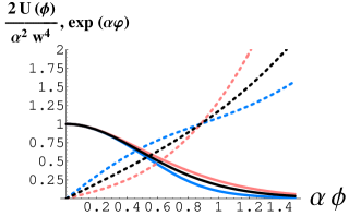
In Fig. 1, the shape of the scalar potential and the development of the volume of the space for the case with and . From this figure, we can see that when the constant is positive, power-law inflation (for large ) is more effective, and when is negative, de Sitter expansion (for small ) is more effective. Of course, from a cosmological perspective, a precise analysis that takes into account cosmic time is necessary, but we believe that such a tendency can be read. Furthermore, since this model ignores the scalar field dependence of , more detailed investigation is necessary in the future.
For the case with constant , the slow-roll parameters are expressed by the single-field prepotential , as
| (60) | |||||
| (61) |
where , and the equation of motion (42) reduces to . Thus, the slow-roll condition is satisfied if and/or and/or . Thus, in the example of the present section, the power-law inflation at tends to satisfy the slow-roll condition, if . When the opposite tendency occurs. This provides a qualitative explanation for what depicted in Fig. 1.
VI Summary and outlook
In this paper, we adopted the quantum version of the BPS equation for a class of gravitating scalar theories, and determined the wave function of the Universe. A very plausible solution that leads to a probability density for scalar fields was found. Instead of choosing the initial conditions of the wave function in the Wheeler–DeWitt equation, the solution is constrained by adopting the BPS equation. In this study, we found that the initial probable value of the scalar fields is given by the maximum of the positive prepotential and the scale factor of the flat space is zero, for an example. In the present analysis, we left aside the problem of operator ordering HP ; TW ; Halliwell2 ; KW ; SH ; HC as well as the positivity of the probability measure.101010The most gentle solution to the interpretation would be to define the expectation value of as . These are issues that remain to be addressed in the future.
Russo Russo2 also considered the general nonlinear sigma model. In that case, further study is required, since we claim that the probability measure of scalar fields is proportional to . Moreover, an interesting future challenge will be to search for a model that fits cosmology within that category.
It is essential to pursue the symmetry that is the origin of the potential shape of the scalar model. Future work should include considering supersymmetry or pseudo-supersymmetry, as well as connections with known supergravity models and theories inspired by string theory. Further, it is known that string theory compactifications naturally lead to slowly varying positive potentials (see HVWW , and references therein) as in the examples in the present paper, so it would be interesting to explore the connection of our models to string theories.
Furthermore, in determining the restrictions to the quantum BPS equation, the process of supersymmetrization of the Wheeler–DeWitt equation itself is important Graham1 ; Graham2 ; OSB ; OPR ; RB ; Moniz . In that case, a fermionic wave function will also appear. In such a system, it seems that ideas like third quantization SC ; KAHS2 ; BW of both bosonic and fermionic wave functions in minisuperspace will become natural, so research in that direction will likely be deepened in the future.
References
- (1) J. J. Halliwell, “Introductory lectures on quantum cosmology”, in: Proceedings of 7th Jerusalem Winter School for Theoretical Physics: Quantum Cosmology and Baby Universes, edited by S. Coleman, J. B. Hartle, T. Piran and S. Weinberg (World Scientific, Singapore, 1991), pp. 159–243. arXiv:0909.2566 [gr-qc].
- (2) C. Kiefer, Quantum Gravity, Int. Ser. Monogr. Phys. Vol. 155 (Clarendon Press, Oxford, 2012).
- (3) C. Kiefer, “Conceptual problems on quantum gravity and quantum cosmology”, ISRN Mathematical Physics 2013 (2013) 509316. arXiv:1401.3578 [gr-qc].
- (4) Y. Kazama and R. Nakayama, “Wave packet in quantum cosmology”, Phys. Rev. D32 (1985) 2500.
- (5) C. Kiefer, “Wave packets in minisuperspace”, Phys. Rev. D38 (1988) 1761.
- (6) C. Kiefer, “Wave packets in quantum cosmology and the cosmological constant”, Nucl. Phys. B341 (1990) 273.
- (7) S. S. Gousheh and H. R. Sepangi, “Wave packets and initial conditions in quantum cosmology”, Phys. Lett. A272 (2000) 304. gr-qc/0006094.
- (8) N. Kan, M. Kuniyasu, K. Shiraishi and K. Takimoto, “Accelerating cosmologies in an integrable model with noncommutative minisuperspace variables”, J. Phys. Comm. 4 (2020) 075010. arXiv:1903.07895 [gr-qc].
- (9) J. G. Russo, “New exact solutions in multi-scalar field cosmology”, JCAP 2307 (2023) 066. arXiv:2304.12360 [gr-qc].
- (10) J. G. Russo, “Phantoms and strange attractors in cosmology”, JCAP 2207 (2022) 015. arXiv:2204.06018 [hep-th].
- (11) D. S. Salopek and J. R. Bond, “Nonlinear evolution of long wavelength metric fluctuations in inflationary models”, Phys. Rev. D42 (1990) 3936.
- (12) D. Bazeia, C. B. Gomes, L. Losano and R. Menezes, “First-order formalism and dark energy”, Phys. Lett. B633 (2006) 415. astro-ph/0601069.
- (13) D. Bazeia, L. Losano, J. J. Rodrigues and R. Rosenfeld, “First-order formalism and dark energy and dust”, Eur. Phys. J. C55 (2008) 113. astro-ph/0611770.
- (14) J. Sadeghi and A. R. Amani, “Deformation of two coupled scalar fields with cosmological solution”, Acta Phys. Polon. A113 (2008) 677.
- (15) J. E. Lidsey, “Cosmology and the Korteweg–de Vries equation”, Phys. Rev. D86 (2012) 123523. arXiv:1205.5641 [astro-ph].
- (16) M. Taylor, “ deformations in general dimensions”, Adv. Theor. Math. Phys. 27 (2023) 37. arXiv:1805.10287 [hep-th].
- (17) R. Graham, “Supersymmetric Bianchi type-IX cosmology”, Phys. Rev. Lett. 67 (1991) 1381.
- (18) R. Graham, “Supersymmetric general Bianchi type IX cosmology with a cosmological term”, Phys. Lett. B277 (1992) 393.
- (19) O. Obregón, J. Socorro and J. Benítez, “Supersymmetric quantum cosmology proposals and the Bianchi type-II model”, Phys. Rev. D47 (1993) 4471.
- (20) O. Obregón, J. Pullin and M. P. Ryan, “Bianchi cosmologies: New variables and a hidden supersymmetry”, Phys. Rev. D48 (1993) 5642. gr-qc/9308001.
- (21) C. Ramírez and V. Vázquez-Báez, “Quantum supersymmetric FRW cosmology with a scalar field”, Phys. Rev. D93 (2016) 043505. arXiv:1511.04425 [gr-qc].
- (22) P. V. Moniz, “Quantum cosmology — the supersymmetric perspective”, vols. 1 and 2, Lect. Notes Phys. 803 and 804 (Springer, Berlin Heidelberg 2010).
- (23) H. Ooguri, C. Vafa and E. Verlinde, “Hartle–Hawking wave-function for flux compactifications: The entropic principle”, Lett. Math. Phys. 74 (2005) 311. hep-th/0502211.
- (24) S. Cecotti and C. Vafa, “Topological–anti-topological fusion”, Nucl. Phys. B367 (1991) 359.
- (25) J. W. York, “Role of conformal three-geometry in the dynamics of gravitation”, Phys. Rev. Lett. 28 (1972) 1082.
- (26) G. W. Gibbons and S. W. Hawking, “Action integrals and partition functions in quantum gravity”, Phys. Rev. D15 (1972) 2752.
- (27) V. Godet, “Quantum cosmology as automorphic dynamics”, arXiv:2405.09833.
- (28) A. Vilenkin, “Quantum cosmology and the initial state of the Universe”, Phys. Rev. D37 (1988) 888.
- (29) A. Vilenkin, “Approach to quantum cosmology”, Phys. Rev. D50 (1994) 2581.
- (30) J. B. Hartle and S. W. Hawking, “Wave function of the universe”, Phys. Rev. D28 (1983) 2960.
- (31) S. W. Hawking, “The quantum state of the universe”, Nucl. Phys. B239 (1984) 257.
- (32) A. Vilenkin, “Boundary conditions in quantum cosmology”, Phys. Rev. D33 (1986) 3560.
- (33) A. Vilenkin, “Interpretation of the wave function of the Universe”, Phys. Rev. D39 (1989) 1116.
- (34) D. He, D. Gao and Q.-y. Cai, “Dynamical interpretation of the wave function of the Universe”, Phys. Lett. B748 (2015) 361. arXiv:1507.06727 [astro-ph].
- (35) I. P. Neupane, “Accelerating cosmologies from exponential potentials”, Class. Quant. Grav. 21 (2004) 4387. hep-th/0311071.
- (36) J. G. Russo, “Exact solution of scalar tensor cosmology with exponential potentials and transient acceleration”, Phys. Lett. B600 (2004) 185. hep-th/0403010.
- (37) E. Elizalde, S. Nojiri and S. D. Odintsov, “Late-time cosmology in (phantom) scalar-tensor theory: dark energy and the cosmic speed-up”, Phys. Rev. D70 (2004) 043539. hep-th/0405034.
- (38) E. Silverstein and D. Tong “Scalar speed limits and cosmology: Acceleration from D-cceleration”, Phys. Rev. D70 (2004) 103505. hep-th/0310221.
- (39) M. Alishahiha, E. Silverstein and D. Tong “DBI in the sky: Non-Gaussianity from inflation with a speed limit”, Phys. Rev. D70 (2004) 123505. hep-th/0404084.
- (40) A. Psinas, “Quantum cosmology aspects of D3 branes and tachyon dynamics”, JHEP 0604 (2006) 042. hep-th/0511270.
- (41) S. W. Hawking and D. N. Page, “Operator ordering and the flatness of the universe”, Nucl. Phys. B264 (1986) 185.
- (42) N. C. Tsamis and R. P. Woodard, “The factor-ordering problem must be reglated”, Phys. Rev. D36 (1987) 3641.
- (43) J. J. Halliwell, “Derivation of the Wheeler-DeWitt equation from a path integral for minisuperspace models”, Phys. Rev. D38 (1988) 2468.
- (44) N. Kontoleon and D. L. Wiltshire, “Operator ordering and consistency of the wave function of the Universe”, Phys. Rev. D59 (1999) 063513. gr-qc/9807075.
- (45) R. Šteigl and F. Hinterleitner, “Factor ordering in standard quantum cosmology”, Class. Quant. Grav. 23 (2006) 3879. gr-qc/0511149.
- (46) D. He and Q.-y Cai, “Duality between operator ordering factor and massless scalar field”, Eur. Phys. J. C82 (2022) 791.
- (47) D. van de Heisteeg, C. Vafa, M. Wiesner and D. H. Wu, “Bounds on field range for slowly varying positive potentials”, JHEP 2402 (2024) 175. arXiv:2305.07701 [hep-th].
- (48) Y.-G. Shen and Z.-Y. Cheng, “Quantization of the Bianchi type universe”, Chin. Astron. Astrophys. 21 (1997) 389.
- (49) N. Kan, T. Aoyama, T. Hasegawa and K. Shiraishi, “Third quantization for scalar and spinor wave functions of the Universe in an extended minisuperspace”, Class. Quant. Grav. 39 (2022) 165010. arXiv:2110.06469 [gr-qc].
- (50) S. Barroso Bellido and F. Wagner, “New guest in the third quantized multiverse”, Phys. Rev. D105 (2022) 106001. arXiv:2203.05387 [gr-qc].