Quantum annealing with pairs of ${}^{2}\Sigma$ molecules as qubits

QA is an optimization algorithm based on the adiabatic theorem of quantum mechanics. The adiabatic theorem ensures that one can prepare a quantum system in the ground state of a desired Hamiltonian ($\hat{H}_{\_}{\rm p}$) from the ground state of a simpler Hamiltonian ($\hat{H}_{\_}{\rm i}$) by a transformation of $\hat{H}_{\_}{\rm i}$ to $\hat{H}_{\_}{\rm p}$. This is possible if the ground state is separated from excited states by a finite energy gap throughout the transformation. In most current implementations of QA [25, 26], a discrete optimization problem is encoded into a graph $G=(V,E)$ with spin-1/2 vertices $V$ and edges $E$ representing an Ising model Hamiltonian:

$$\hat{H}_{\_}{\rm IM}=\sum_{\_}{i\in V}h_{\_}i\sigma^{z}_{\_}i+\sum_{\_}{(i,j)\in E}J_{\_}{ij}\sigma^{z}_{\_}i\sigma^{z}_{\_}j$$

(1)

where $h_{\_}i$ is the bias applied to spin $i$, $J_{\_}{ij}$ is the Ising coupling between spins $i$ and $j$, and $\sigma^{z}_{\_}i$ is the Pauli Z matrix applied to the $i$th spin. Encoding an optimization problem into an Ising model involves determining a suitable graph of spins, which is, in itself, an NP-hard problem [25].

Given this encoding ($\hat{H}_{\_}{\rm p}=\hat{H}_{\_}{\rm IM}$), the spin system is initialized in the ground state of the following Hamiltonian $\hat{H}_{\_}{\rm i}$:

$$\hat{H}_{\_}{\rm i}=\sum_{\_}{i\in V}^{n}\sigma^{x}_{\_}i$$

(2)

where $\sigma^{x}_{\_}i$ is the Pauli X matrix applied to the $i$th spin. The ground state of Hamiltonian (2) is an equal superposition of all possible spin states. To allow adiabatic transformation of the ground state of $\hat{H}_{\_}{\rm i}$ into the ground state of $\hat{H}_{\_}{\rm p}$, a physical system must realize a TFIM with tunable parameters,

$$\hat{H}_{\_}{\rm TFIM}(s)=\sum_{\_}{i\in V}h_{\_}i(s)\sigma^{z}_{\_}i+\Delta_{\_}i(s)\sigma^{x}_{\_}i+\sum_{\_}{(i,j)\in E}J_{\_}{ij}(s)\sigma^{z}_{\_}i\sigma^{z}_{\_}j$$

(3)

where $s$ is the annealing parameter varying from 0 to 1 during the annealing and $\Delta_{\_}i$ is the transverse field strength for spin $i$. The Hamiltonian parameters must be functions of the annealing parameter with the following limits:

$$s:0\rightarrow 1:\begin{cases}h_{\_}i(s):0\rightarrow h_{\_}i\\ J_{\_}{ij}(s):0\rightarrow J_{\_}{ij}\\ \Delta_{\_}i(s):1\rightarrow 0\\ \end{cases}.$$

(4)

Hamiltonian (1) is diagonal in the $\sigma^{z}$ basis so the ground state of $\hat{H}_{\_}{\rm p}$ can be determined by measuring the spin configuration at $s=1$, which gives the solution to the optimization problem at hand.

The Hamiltonian for a ${}^{2}\Sigma$ radical in the vibrational ground state placed in a superposition of dc electric $\bm{E}$ and magnetic $\bm{B}$ fields can be written as

$$\hat{H}=B_{\_}e\bm{N}^{2}+\gamma_{\_}{SR}\bm{N}\cdot\bm{S}-\bm{E}\cdot\bm{d}+\mu_{\_}Bg_{\_}S\bm{B}\cdot\bm{S}$$

(5)

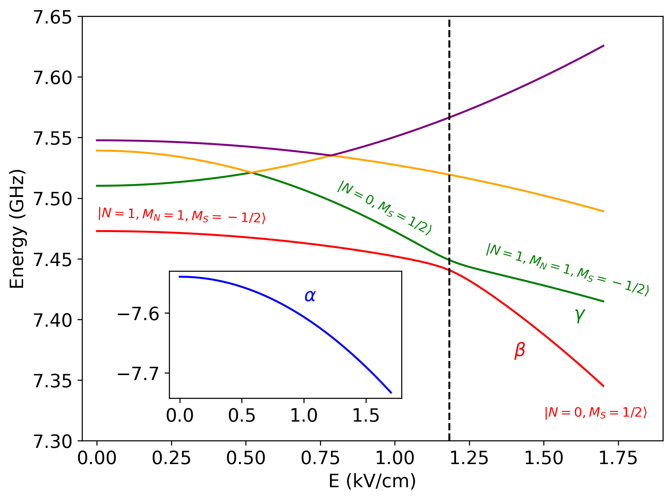
where $B_{\_}e$ is the rotational constant, $\gamma_{\_}{SR}$ is the spin-rotational interaction constant, $\bm{N}$ and $\bm{S}$ are the rotational and spin angular momenta of the molecule, $\bm{d}$ is the dipole moment of the molecule, $\mu_{\_}B$ is the Bohr magneton, and $g_{\_}S$ is the electron spin $g$ factor. For simplicity, we assume that the magnetic- and electric-field vectors are co-aligned. Figure 1 shows the lowest five energy levels of SrF($X^{2}\Sigma^{+}$) corresponding to $N=0$ and 1. The state labeled $\alpha$ is predominantly $\lvert N=0,M_{\_}S=-1/2\rangle$, whereas the states labeled $\beta$ and $\gamma$ exhibit an avoided crossing, with $\beta$ changing from $\lvert N=1,M_{\_}N=1,M_{\_}S=-1/2\rangle$ to $\lvert N=0,M_{\_}S=1/2\rangle$ and $\gamma$ undergoing the reverse change, as the field magnitude is increased.

Encoding a spin-1/2 system into two isolated eigenstates of a single molecule and allowing for dipole-dipole interactions [76] leads to the following many-body Hamiltonian [77] (assuming the energy difference between the two spin-rotational states is much larger in magnitude than the intermolecular interactions):

$$\hat{H}=\sum_{\_}ih_{\_}i\hat{S}_{\_}i^{z}+\frac{1}{2}\sum_{\_}{i\neq j}\left[\frac{J_{\_}{\perp_{\_}{ij}}}{2}\left(\hat{S}_{\_}i^{+}\hat{S}_{\_}j^{-}+{\rm h.c.}\right)+J_{\_}{z_{\_}{ij}}\hat{S}_{\_}i^{z}\hat{S}_{\_}j^{z}\right].$$

(6)

Appendix A outlines the derivation of Eq. (6). With $\lvert\uparrow\rangle=\lvert\beta\rangle$ and $\lvert\downarrow\rangle=\lvert\gamma\rangle$, the dependence of $J_{\_}\perp$ and $J_{\_}z$ on the electric-field magnitude produces three regimes of spin models illustrated in Fig. 2 for two molecules (SrF and SrI) in the $X^{2}\Sigma^{+}$ state. Near the avoided crossing, the spin-exchange interaction dominates as $J_{\_}\perp\gg J_{\_}z$, yielding a quantum $XY$ spin model ($XXZ$ model with $J_{\_}z=0$). At electric fields far detuned from the avoided crossing, the Ising coupling dominates as $J_{\_}z\gg J_{\_}\perp$, reducing the Hamiltonian to a quantum Ising model. At electric fields between these two extremes, both couplings are similar in value. We define $E_{\_}\perp(B)$ to be the electric-field magnitude at which $J_{\_}\perp$ is maximized and $E_{\_}z(B)$ can be assigned to be any electric-field magnitude at which $J_{\_}z\gg J_{\_}\perp$.

The coupling between molecules also depends on the angle between the intermolecular axis and the field directions following the anisotropy of dipole-dipole interactions (see Appendix A). While Fig. 2 displays the couplings for two molecules with an intermolecular axis perpendicular to the electric and magnetic fields ($\theta=\pi/2$), the couplings are modulated by Eq. (17) for other values of $\theta$. We define ferromagnetic and anti-ferromagnetic interactions between molecules with negative and positive signs on $J_{\_}z$ respectively. Therefore, at $\theta=\pi/2$, interactions between molecules are anti-ferromagnetic ($J_{\_}z\geq 0$), and when the intermolecular axis is parallel to the fields ($\theta=0$) the interactions are ferromagnetic ($J_{\_}z\leq 0$) and twice as large in magnitude as the perpendicular case.

Model (6) is not suitable for QA, as it conserves the number of spin excitations. The TFIM model of Eq. (3) includes the transverse field terms $\sigma_{\_}i^{x}$, which generate spin excitations during the annealing. It is possible to engineer $\sigma_{\_}i^{x}$ terms by coupling the $\lvert\uparrow\rangle$ and $\lvert\downarrow\rangle$ states of the individual molecules with near-resonant MW fields. However, the biases of the qubits $h_{\_}i$ depend on the detuning of the MW field from the energy differences between the $\lvert\uparrow\rangle$ and $\lvert\downarrow\rangle$ states of each molecule. In order to realize an Ising model with arbitrary biases encoding an optimization problem, it may be necessary to apply multiple dressing fields for the corresponding biases on each qubit. The frequencies of these dressing fields must be tuned simultaneously to achieve transformation (4). Even in simple cases with homogeneous fields and zero biases, the $\lvert\uparrow\rangle$ – $\lvert\downarrow\rangle$ energy gaps are modified by the molecular interactions (Eq. (18)) and the resonant frequencies vary between the qubits. QA with molecules dressed by MW fields as qubits thus appears to be a very complex task.

To overcome this problem, we consider pairs of molecules exchanging an excitation as qubits of a many-body Hamiltonian. This encoding scheme does not require any MW fields and allows tuning of qubit parameters and couplings by varying a single dc field, electric or magnetic. It may, however, require complicated geometry of the trapping optical lattice and precise control of the field gradients.

Within the subspace spanned by the $\lvert\uparrow\downarrow\rangle$ and $\lvert\downarrow\uparrow\rangle$ states, the isolated two-molecule system encodes a spin-1/2 qubit with the following Hamiltonian:

$$\hat{H}_{\_}q=h_{\_}q\hat{S}_{\_}q^{z}+\Delta_{\_}q\hat{S}_{\_}q^{x},$$

(7)

where

	$\displaystyle h_{\_}q$	$\displaystyle=h_{\_}1-h_{\_}2,$	$\displaystyle\Delta_{\_}q$	$\displaystyle=J_{\_}\perp,$		(8)
	$\displaystyle S_{\_}q^{x}$	$\displaystyle=\frac{1}{2}\begin{pmatrix}0&1\\ 1&0\end{pmatrix},$	$\displaystyle S_{\_}q^{z}$	$\displaystyle=\frac{1}{2}\begin{pmatrix}1&0\\ 0&-1\end{pmatrix}$		(9)

in the basis:

$\displaystyle\lvert\uparrow\downarrow\rangle=\lvert 0\rangle$

$\displaystyle=\begin{pmatrix}1\\ 0\end{pmatrix}$

$\displaystyle\lvert\downarrow\uparrow\rangle=\lvert 1\rangle$

$\displaystyle=\begin{pmatrix}0\\ 1\end{pmatrix}$

The bias of the qubit ($h_{\_}q$) is the difference in the energy gap of the $\lvert\uparrow\rangle$ and $\lvert\downarrow\rangle$ states of the two molecules, which can be tuned by applying a gradient to the electric-field magnitude. The transverse field parameter of the qubit ($\Delta_{\_}q$) depends on the magnitude of the fields and the orientation of the fields. However, for this parameter to be relevant, one must ensure that $h_{\_}1-h_{\_}2\approx\Delta_{\_}q$. We consider the following field configurations for the two molecules of each qubit: $B=B_{\_}1=B_{\_}2$ and $E_{\_}1=E_{\_}2-\delta E$ with $\delta E\ll E_{\_}1,E_{\_}2$. Qubit bias can also be set using a single molecule locked in one of the two states $\lvert\uparrow\rangle$ or $\lvert\downarrow\rangle$ and coupled to the qubit. This makes one of the two states more favorable energetically and has the added benefits of being of the same order of magnitude as the inter-qubit couplings, which can be easily accommodated in the annealing procedure described below. Hereafter, ‘qubit’ refers to the two-molecule system with Hamiltonian (7).

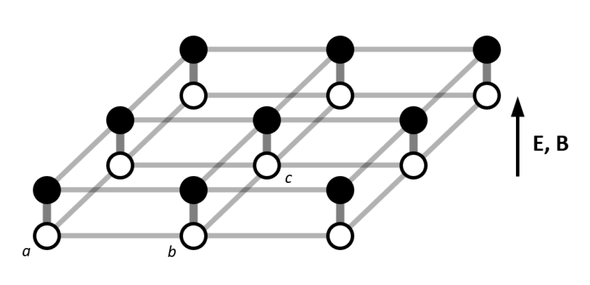
The two-qubit Hamiltonian for four molecules in a rectangular configuration (Fig. 3 top) with molecules 1 and 2 forming qubit $a$ and molecules 3 and 4 forming qubit $b$ is

	$\displaystyle\hat{H}$	$\displaystyle=\hat{H}_{\_}a+\hat{H}_{\_}b+J_{\_}{z_{\_}{13}}S_{\_}1^{z}S_{\_}3^{z}+J_{\_}{z_{\_}{24}}S_{\_}2^{z}S_{\_}4^{z}$
		$\displaystyle+J_{\_}{z_{\_}{14}}S_{\_}1^{z}S_{\_}4^{z}+J_{\_}{z_{\_}{23}}S_{\_}2^{z}S_{\_}3^{z}$
		$\displaystyle+\frac{J_{\_}{\perp_{\_}{13}}}{2}\left(S_{\_}1^{+}S_{\_}3^{-}+{\rm h.c.}\right)+\frac{J_{\_}{\perp_{\_}{24}}}{2}\left(S_{\_}2^{+}S_{\_}4^{-}+{\rm h.c.}\right)$
		$\displaystyle+\frac{J_{\_}{\perp_{\_}{14}}}{2}\left(S_{\_}1^{+}S_{\_}4^{-}+{\rm h.c.}\right)+\frac{J_{\_}{\perp_{\_}{23}}}{2}\left(S_{\_}2^{+}S_{\_}3^{-}+{\rm h.c.}\right)$		(10)

where $\hat{H}_{\_}a$ and $\hat{H}_{\_}b$ are given by Eq. (7). The spin-exchange dynamics induced by $J_{\_}{\perp_{\_}{ij}}$ will take qubit states outside of the Hilbert space of the $\lvert 0\rangle$ and $\lvert 1\rangle$ states of each qubit (e.g. pairs of molecules within a qubit may end up in states $\lvert\uparrow\uparrow\rangle$ and $\lvert\downarrow\downarrow\rangle$). These interactions can be suppressed by placing the qubits further apart or detuning the qubits so that $|h_{\_}1-h_{\_}3|\gg|J_{\_}{\perp_{\_}{13}}|$ and $|h_{\_}2-h_{\_}4|\gg|J_{\_}{\perp_{\_}{24}}|$. This can be achieved by placing qubits in different fields by applying a gradient of an electric or magnetic field along the direction joining the qubits. In this limit, the Hamiltonian reduces to

$$\hat{H}=h_{\_}a\hat{S}_{\_}a^{z}+\Delta_{\_}a\hat{S}_{\_}a^{x}+h_{\_}b\hat{S}_{\_}b^{z}+\Delta_{\_}b\hat{S}_{\_}b^{x}\pm J_{\_}{ab}S_{\_}a^{z}S_{\_}b^{z}$$

(11)

where $J_{\_}{ab}=J_{\_}{z_{\_}{13}}+J_{\_}{z_{\_}{24}}-J_{\_}{z_{\_}{14}}-J_{\_}{z_{\_}{23}}$, and the sign of the last term depends on the encoding of the qubits (positive when $\lvert 0_{\_}a\rangle=\lvert\uparrow_{\_}1\downarrow_{\_}2\rangle$, $\lvert 1_{\_}a\rangle=\lvert\downarrow_{\_}1\uparrow_{\_}2\rangle$ and $\lvert 0_{\_}b\rangle=\lvert\uparrow_{\_}3\downarrow_{\_}4\rangle$, $\lvert 1_{\_}b\rangle=\lvert\downarrow_{\_}3\uparrow_{\_}4\rangle$ and negative when one of the qubits is inverted as in $\lvert 0_{\_}b\rangle=\lvert\downarrow_{\_}3\uparrow_{\_}4\rangle$, $\lvert 1_{\_}b\rangle=\lvert\uparrow_{\_}3\downarrow_{\_}4\rangle$). We define ferromagnetic and anti-ferromagnetic interactions between molecules as having negative and positive signs on the $J_{\_}{ab}$ couplings respectively. The setup illustrated in the top panel of Fig. 3 has anti-ferromagnetic couplings between the qubits, while also having ferromagnetic couplings between the molecules within each qubit.

Qubits stacked head to head have the same Hamiltonian with half the inter-qubit interaction strength. Other stacking configurations can also lead to interesting coupling interplays. For example, qubits stacked perpendicularly on top of each other (in a cross shape with one qubit lying on the symmetry plane of the other qubit) would be completely decoupled from each other and configurations with asymmetric interactions on the molecules of a single qubit can lead to non-zero bias terms.

Couplings between qubits are also dependent on the field magnitudes, with stronger fields resulting in stronger couplings. For SrF molecules considered here, Ising couplings between two qubits can be tuned within the range 300-2500 Hz with magnetic fields of 540-620 mT and dc electric fields of 1.6-8.5 kV/cm ($E_{\_}z(B)$) on each qubit. Electric- and magnetic-field gradients and masks could allow for this wide range of couplings between qubits in a single connected system. Combined with the anisotropy of the dipole-dipole interactions and the resulting qubit-qubit couplings, many different Ising models can be encoded into molecules.

The present method of encoding qubits can be very sensitive to inhomogeneities of external magnetic and electric fields. Field perturbations may induce significant modifications of the energy differences between the $\beta$ and $\gamma$ states, given by $h_{\_}1$ and $h_{\_}2$ in Eq. (8). Therefore, variations in the field magnitudes applied to a pair of molecules comprising a qubit could lead to significant changes in the bias of the qubit. This effect also hinders the spin-exchange interactions essential to the transverse field simulation of the system so care must be taken to ensure field homogeneity over length scales of individual qubits. However, small perturbations of the fields between the qubits should not be problematic as these would only slightly modify the couplings and could even be desirable, as they diminish the effect of unwanted spin-exchange interactions between qubits.

Hamiltonian (11) is the transverse field Ising model used in QA applications. In order to use this system as a quantum annealer, one needs to be able to transform

$$\hat{H}_{\_}{\rm i}=\Delta_{\_}a\hat{S}_{\_}a^{x}+\Delta_{\_}b\hat{S}_{\_}b^{x}$$

(12)

to

$$\hat{H}_{\_}{\rm f}=h_{\_}a\hat{S}_{\_}a^{z}+h_{\_}b\hat{S}_{\_}b^{z}+J_{\_}zS_{\_}a^{z}S_{\_}b^{z}$$

(13)

by tuning a single external field parameter. The sensitivity of states $\beta$ and $\gamma$ to external fields near the avoided crossing shown in Fig. 2 makes this possible.

When the qubits are initialized in a superposition of $\lvert\uparrow\downarrow\rangle$ and $\lvert\downarrow\uparrow\rangle$ states at ($E_{\_}{\perp_{\_}a}$, $B_{\_}a$, $\delta E_{\_}a=0$) and ($E_{\_}{\perp_{\_}b}$, $B_{\_}b$, $\delta E_{\_}b=0$), the Hamiltonian of the two-qubit system is given by Eq. (12) with the values of $\Delta_{\_}a$ and $\Delta_{\_}b$ determined by the field magnitudes at each qubit. Increasing the electric-field strength to $E_{\_}{z_{\_}i}$ decreases the magnitude of $\Delta$, while increasing $|\delta E_{\_}i|$ increases $|h_{\_}i|$. The final Hamiltonian of two qubits at ($E_{\_}{z_{\_}a}$, $B_{\_}a$, $\delta E_{\_}a$) and ($E_{\_}{z_{\_}b}$, $B_{\_}b$, $\delta E_{\_}b$) becomes (13) where the values of $h_{\_}a$ and $h_{\_}b$ are determined by $\delta E$, and $J_{\_}z$ is determined by the field magnitudes at each qubit. For SrF, $\delta E\approx 10$ V/m generates a bias comparable to the Ising coupling between qubits placed 1000 nm apart. Alternatively, $h_{\_}a$ and $h_{\_}b$ can also be modified by coupling each qubit to a molecule locked in either $\beta$ or $\gamma$ (detuning the fields away from the avoided crossing locks the molecule in one of these two states). In this case, increasing the electric-field strength at each qubit from $E_{\_}{\perp_{\_}i}$ to $E_{\_}{z_{\_}i}$ also increases the magnitude of $h_{\_}a$ and $h_{\_}b$. The final values of $h_{\_}a$ and $h_{\_}b$ can be calculated considering the couplings between the biasing molecules and qubits.

Initialization and read-out of the system can be done by resonant microwave excitation in a gradient of an electric field, as proposed by DeMille [50]. Electric-field gradients used for this purpose are similar in magnitude to the electric fields needed to apply a bias on the qubits considered here. In our examples using SrF, this can be done with field gradients $\approx 1$ kV/cm².

In the following discussion, we define the valid qubit states as the collection of states with a single excitation in each qubit. In the subspace of valid qubit states, any measurement (in the $\lvert\uparrow\rangle$ and $\lvert\downarrow\rangle$ basis) leads to a qubit state of $\lvert 0\rangle$ and $\lvert 1\rangle$ for all qubits. Conversely, invalid states are measured states of the system that do not correspond to any 0-1 qubit encoding described above. These states are a result of the spin-exchange interactions of molecules in different qubits resulting in pairs of molecules in $\lvert\uparrow\uparrow\rangle$ or $\lvert\downarrow\downarrow\rangle$ states. The probability of obtaining such states is amplified by favorable ferromagnetic couplings between molecules in different qubits.

For QA applications, the goal is to find the minimum-energy state in the subspace of valid qubit states. In some configurations (e.g. when the intraqubit molecular interactions are ferromagnetic), the final ground state of the system (in the subspace of states with $n/2$ excitations for $n$ molecules) after annealing is an invalid state. Thus, the annealing transformation should be quasi-adiabatic and annealing times need to be carefully tuned to balance the adiabaticity of the evolution, while limiting the undesired spin-exchange interactions between qubits. Generally, in configurations where the intraqubit Ising couplings are ferromagnetic, we expect to have a larger probability of observing invalid states.

In order to test the annealing procedure with different configurations of molecular ensembles, we use quantum dynamics simulations of the corresponding spin-1/2 $XXZ$ Hamiltonian (6) in a time-dependent electric field with the QuTip python package [78, 79]. We assume that the probability of populating any state other than $\lvert\beta\rangle$ and $\lvert\gamma\rangle$ is negligible. This is a reasonable assumption as these states are separated from other states by a significant energy gap. For example, in the case of SrF molecules depicted in Fig. 1, these states are separated from other states by $>0.1$ GHz, while the relevant coupling strengths are $<1$ MHz and the time scale of QA is $\approx 10$ ms. Each system is initialized in an equal superposition of valid qubit states. Qubits with ferromagnetic couplings between molecules within qubits need to be initialized in the $\lvert 0\rangle+\lvert 1\rangle$ state and those with anti-ferromagnetic couplings need to be initialized in the $\lvert 0\rangle-\lvert 1\rangle$ state. Evolution of this initial state during annealing is then calculated by numerical integration of the time-dependent Schrödinger equation using the Adams-Moulton method (implicit Adams) [80] in a variable-coefficient ordinary differential equation solver [81] with a maximum order of 12, using a locally time-independent Hamiltonian in each time step. For our calculations, we used 200 time steps for the one-dimensional (1D) lattice and 100 time steps for the 2D lattice.

References

- Kadowaki and Nishimori [1998] T. Kadowaki and H. Nishimori, Quantum annealing in the transverse ising model, Phys. Rev. E 58, 5355 (1998).
- Harvardla et al. [1994] A. Harvardla, M. Gomez, C. Sebenik, C. Stenson, and J. Doll, Quantum annealing: A new method for minimizing multidimensional functions, Chem. Phys. Lett. 219, 343 (1994).
- Hogg [2000] T. Hogg, Quantum search heuristics, Phys. Rev. A 61, 052311 (2000).
- Farhi et al. [2001a] E. Farhi, J. Goldstone, S. Gutmann, J. Lapan, A. Lundgren, and D. Preda, A quantum adiabatic evolution algorithm applied to random instances of an np-complete problem, Science 292, 472 (2001a).
- Barahona [1982] F. Barahona, On the computational complexity of ising spin glass models, J. Phys. A: Math. Gen. 15, 3241 (1982).
- las Cuevas and Cubitt [2016] G. D. las Cuevas and T. S. Cubitt, Simple universal models capture all classical spin physics, Science 351, 1180 (2016).
- Neven et al. [2009] H. Neven, V. S. Denchev, G. Rose, and W. G. Macready, Training a large scale classifier with the quantum adiabatic algorithm, arXiv preprint arXiv:0912.0779 (2009).
- Babbush et al. [2014] R. Babbush, P. J. Love, and A. Aspuru-Guzik, Adiabatic quantum simulation of quantum chemistry, Sci. Rep. 4, 6603 (2014).
- Hernandez and Aramon [2017] M. Hernandez and M. Aramon, Enhancing quantum annealing performance for the molecular similarity problem, Quantum Inf. Process. 16, 133 (2017).
- Lloyd et al. [2013] S. Lloyd, M. Mohseni, and P. Rebentrost, Quantum algorithms for supervised and unsupervised machine learning, arXiv preprint arXiv:1307.0411 (2013).
- Benedetti et al. [2017] M. Benedetti, J. Realpe-Gómez, R. Biswas, and A. Perdomo-Ortiz, Quantum-assisted learning of hardware-embedded probabilistic graphical models, Phys. Rev. X 7, 041052 (2017).
- Li et al. [2018] R. Y. Li, R. Di Felice, R. Rohs, and D. A. Lidar, Quantum annealing versus classical machine learning applied to a simplified computational biology problem, NPJ Quantum Inf. 4, 1 (2018).
- Garnerone et al. [2012] S. Garnerone, P. Zanardi, and D. A. Lidar, Adiabatic quantum algorithm for search engine ranking, Phys. Rev, Lett. 108, 230506 (2012).
- Perdomo-Ortiz et al. [2012] A. Perdomo-Ortiz, N. Dickson, M. Drew-Brook, G. Rose, and A. Aspuru-Guzik, Finding low-energy conformations of lattice protein models by quantum annealing, Sci. Rep. 2, 1 (2012).
- Rosenberg et al. [2016] G. Rosenberg, P. Haghnegahdar, P. Goddard, P. Carr, K. Wu, and M. L. De Prado, Solving the optimal trading trajectory problem using a quantum annealer, IEEE Journal of Selected Topics in Signal Processing 10, 1053 (2016).
- Perdomo-Ortiz et al. [2015] A. Perdomo-Ortiz, J. Fluegemann, S. Narasimhan, R. Biswas, and V. N. Smelyanskiy, A quantum annealing approach for fault detection and diagnosis of graph-based systems, Eur. Phys. J.: Spec. Top. 224, 131 (2015).
- Perdomo-Ortiz et al. [2019] A. Perdomo-Ortiz, A. Feldman, A. Ozaeta, S. V. Isakov, Z. Zhu, B. O’Gorman, H. G. Katzgraber, A. Diedrich, H. Neven, J. de Kleer, B. Lackey, and R. Biswas, Readiness of quantum optimization machines for industrial applications, Phys. Rev. Appl. 12, 014004 (2019).
- Rieffel et al. [2015] E. G. Rieffel, D. Venturelli, B. O’Gorman, M. B. Do, E. M. Prystay, and V. N. Smelyanskiy, A case study in programming a quantum annealer for hard operational planning problems, Quantum Inf. Process. 14, 1 (2015).
- Venturelli et al. [2015] D. Venturelli, D. J. Marchand, and G. Rojo, Quantum annealing implementation of job-shop scheduling, arXiv preprint arXiv:1506.08479 (2015).
- Khoshaman et al. [2018] A. Khoshaman, W. Vinci, B. Denis, E. Andriyash, H. Sadeghi, and M. H. Amin, Quantum variational autoencoder, Quantum Sci. Technol. 4, 014001 (2018).
- Wilson et al. [2021] M. Wilson, T. Vandal, T. Hogg, and E. G. Rieffel, Quantum-assisted associative adversarial network: Applying quantum annealing in deep learning, Quantum Machine Intelligence 3, 1 (2021).
- Mott et al. [2017] A. Mott, J. Job, J.-R. Vlimant, D. Lidar, and M. Spiropulu, Solving a higgs optimization problem with quantum annealing for machine learning, Nature 550, 375 (2017).
- Das et al. [2019] S. Das, A. J. Wildridge, S. B. Vaidya, and A. Jung, Track clustering with a quantum annealer for primary vertex reconstruction at hadron colliders, arXiv preprint arXiv:1903.08879 (2019).
- Preskill [2018] J. Preskill, Quantum Computing in the NISQ era and beyond, Quantum 2, 79 (2018).
- McGeoch [2020] C. C. McGeoch, Theory versus practice in annealing-based quantum computing, Theor. Comput. Sci. 816, 169 (2020).
- Boothby et al. [2021] K. Boothby, C. Enderud, T. Lanting, R. Molavi, N. Tsai, M. H. Volkmann, F. Altomare, M. H. Amin, M. Babcock, A. J. Berkley, C. B. Aznar, M. Boschnak, H. Christiani, S. Ejtemaee, B. Evert, M. Gullen, M. Hager, R. Harris, E. Hoskinson, J. P. Hilton, K. Jooya, A. Huang, M. W. Johnson, A. D. King, E. Ladizinsky, R. Li, A. MacDonald, T. M. Fernandez, R. Neufeld, M. Norouzpour, T. Oh, I. Ozfidan, P. Paddon, I. Perminov, G. Poulin-Lamarre, T. Prescott, J. Raymond, M. Reis, C. Rich, A. Roy, H. S. Esfahani, Y. Sato, B. Sheldan, A. Smirnov, L. J. Swenson, J. Whittaker, J. Yao, A. Yarovoy, and P. I. Bunyk, Architectural considerations in the design of a third-generation superconducting quantum annealing processor (2021), arXiv:2108.02322 [quant-ph] .
- Micheli et al. [2006] A. Micheli, G. Brennen, and P. Zoller, A toolbox for lattice spin models with polar molecules, Nat. Phys. 2, 341 (2006).
- Gorshkov et al. [2011a] A. V. Gorshkov, S. R. Manmana, G. Chen, J. Ye, E. Demler, M. D. Lukin, and A. M. Rey, Tunable superfluidity and quantum magnetism with ultracold polar molecules, Phys. Rev. Lett. 107, 115301 (2011a).
- Gorshkov et al. [2011b] A. V. Gorshkov, S. R. Manmana, G. Chen, E. Demler, M. D. Lukin, and A. M. Rey, Quantum magnetism with polar alkali-metal dimers, Phys. Rev. A 84, 033619 (2011b).
- Sundar et al. [2018] B. Sundar, B. Gadway, and K. Hazzard, Synthetic dimensions in ultracold polar molecules, Sci. Rep. 8, 3422 (2018).
- Gadway and Yan [2016] B. Gadway and B. Yan, Strongly interacting ultracold polar molecules, J. Phys. B: At. Mol. Opt. Phys. 49, 152002 (2016).
- Büchler et al. [2007] H. P. Büchler, A. Micheli, and P. Zoller, Three-body interactions with cold polar molecules, Nat. Phys. 3, 726 (2007).
- Weimer [2013] H. Weimer, Quantum simulation of many-body spin interactions with ultracold polar molecules, Mol. Phys. 111, 1753 (2013).
- Hazzard et al. [2014a] K. R. A. Hazzard, M. van den Worm, M. Foss-Feig, S. R. Manmana, E. G. Dalla Torre, T. Pfau, M. Kastner, and A. M. Rey, Quantum correlations and entanglement in far-from-equilibrium spin systems, Phys. Rev. A 90, 063622 (2014a).
- Hazzard et al. [2014b] K. R. A. Hazzard, B. Gadway, M. Foss-Feig, B. Yan, S. A. Moses, J. P. Covey, N. Y. Yao, M. D. Lukin, J. Ye, D. S. Jin, and A. M. Rey, Many-body dynamics of dipolar molecules in an optical lattice, Phys. Rev. Lett. 113, 195302 (2014b).
- de Paz et al. [2013] A. de Paz, A. Sharma, A. Chotia, E. Maréchal, J. H. Huckans, P. Pedri, L. Santos, O. Gorceix, L. Vernac, and B. Laburthe-Tolra, Nonequilibrium quantum magnetism in a dipolar lattice gas, Phys. Rev. Lett. 111, 185305 (2013).
- Gorshkov et al. [2013] A. V. Gorshkov, K. R. Hazzard, and A. M. Rey, Kitaev honeycomb and other exotic spin models with polar molecules, Mol. Phys. 111, 1908 (2013).
- Covey et al. [2018] J. P. Covey, S. A. Moses, J. Ye, and D. S. Jin, Chapter 11 controlling a quantum gas of polar molecules in an optical lattice, in Cold Chemistry: Molecular Scattering and Reactivity Near Absolute Zero (The Royal Society of Chemistry, Cambridge, UK, 2018) pp. 537–578.
- Blackmore et al. [2018] J. A. Blackmore, L. Caldwell, P. D. Gregory, E. M. Bridge, R. Sawant, J. Aldegunde, J. Mur-Petit, D. Jaksch, J. M. Hutson, B. E. Sauer, M. R. Tarbutt, and S. L. Cornish, Ultracold molecules for quantum simulation: rotational coherences in CaF and RbCs, Quantum Sci. Technol. 4, 014010 (2018).
- Rosson et al. [2020] P. Rosson, M. Kiffner, J. Mur-Petit, and D. Jaksch, Characterizing the phase diagram of finite-size dipolar bose-hubbard systems, Phys. Rev. A 101, 013616 (2020).
- Herrera and Krems [2011] F. Herrera and R. V. Krems, Tunable holstein model with cold polar molecules, Phys. Rev. A 84, 051401(R) (2011).
- Dawid et al. [2018] A. Dawid, M. Lewenstein, and M. Tomza, Two interacting ultracold molecules in a one-dimensional harmonic trap, Phys. Rev. A 97, 063618 (2018).
- Xiang et al. [2012] P. Xiang, M. Litinskaya, and R. V. Krems, Tunable exciton interactions in optical lattices with polar molecules, Phys. Rev. A 85, 061401(R) (2012).
- Kruckenhauser et al. [2020] A. Kruckenhauser, L. M. Sieberer, L. De Marco, J.-R. Li, K. Matsuda, W. G. Tobias, G. Valtolina, J. Ye, A. M. Rey, M. A. Baranov, and P. Zoller, Quantum many-body physics with ultracold polar molecules: Nanostructured potential barriers and interactions, Phys. Rev. A 102, 023320 (2020).
- Büchler et al. [2007] H. P. Büchler, E. Demler, M. Lukin, A. Micheli, N. Prokof’ev, G. Pupillo, and P. Zoller, Strongly correlated 2d quantum phases with cold polar molecules: Controlling the shape of the interaction potential, Phys. Rev. Lett. 98, 060404 (2007).
- Brennen et al. [2007] G. K. Brennen, A. Micheli, and P. Zoller, Designing spin-1 lattice models using polar molecules, New J. Phys. 9, 138 (2007).
- Wall et al. [2015a] M. L. Wall, K. Maeda, and L. D. Carr, Realizing unconventional quantum magnetism with symmetric top molecules, New J. Phys. 17, 025001 (2015a).
- Olaya-Agudelo et al. [2019] V. C. Olaya-Agudelo, S. García-Negrete, and K. Rodríguez-Ramírez, Single-excitation correlation dynamics of polar molecules on 1d lattices: driving by external electric fields, Materials Today: Proceedings 14, 134 (2019).
- Kaufman and Ni [2021] A. M. Kaufman and K.-K. Ni, Quantum science with optical tweezer arrays of ultracold atoms and molecules, Nat. Phys. 17, 1324 (2021).
- DeMille [2002] D. DeMille, Quantum computation with trapped polar molecules, Phys. Rev. Lett. 88, 067901 (2002).
- Yelin et al. [2006] S. F. Yelin, K. Kirby, and R. Côté, Schemes for robust quantum computation with polar molecules, Phys. Rev. A 74, 050301(R) (2006).
- Hughes et al. [2020] M. Hughes, M. D. Frye, R. Sawant, G. Bhole, J. A. Jones, S. L. Cornish, M. R. Tarbutt, J. M. Hutson, D. Jaksch, and J. Mur-Petit, Robust entangling gate for polar molecules using magnetic and microwave fields, Phys. Rev. A 101, 062308 (2020).
- Mishima and Yamashita [2009] K. Mishima and K. Yamashita, Quantum computing using rotational modes of two polar molecules, Chem. Phys. 361, 106 (2009).
- Zhu et al. [2013] J. Zhu, S. Kais, Q. Wei, D. Herschbach, and B. Friedrich, Implementation of quantum logic gates using polar molecules in pendular states, J. Chem. Phys. 138, 024104 (2013).
- Mur-Petit et al. [2013] J. Mur-Petit, J. Pérez-Ríos, J. Campos-Martínez, M. I. Hernández, S. Willitsch, and J. J. García-Ripoll, Toward a molecular ion qubit, in Architecture and Design of Molecule Logic Gates and Atom Circuits, edited by N. Lorente and C. Joachim (Springer Berlin Heidelberg, Berlin, Heidelberg, 2013) pp. 267–277.
- Sawant et al. [2020] R. Sawant, J. A. Blackmore, P. D. Gregory, J. Mur-Petit, D. Jaksch, J. Aldegunde, J. M. Hutson, M. R. Tarbutt, and S. L. Cornish, Ultracold polar molecules as qudits, New J. Phys. 22, 013027 (2020).
- Gregory et al. [2021] P. D. Gregory, J. A. Blackmore, S. L. Bromley, J. M. Hutson, and S. L. Cornish, Robust storage qubits in ultracold polar molecules, Nat. Phys. 17, 1149 (2021).
- Karra et al. [2016] M. Karra, K. Sharma, B. Friedrich, S. Kais, and D. Herschbach, Prospects for quantum computing with an array of ultracold polar paramagnetic molecules, J. Chem. Phys. 144, 094301 (2016).
- Müller et al. [2011] M. M. Müller, D. M. Reich, M. Murphy, H. Yuan, J. Vala, K. B. Whaley, T. Calarco, and C. P. Koch, Optimizing entangling quantum gates for physical systems, Phys. Rev. A 84, 042315 (2011).
- Anderegg et al. [2019] L. Anderegg, L. W. Cheuk, Y. Bao, S. Burchesky, W. Ketterle, K.-K. Ni, and J. M. Doyle, An optical tweezer array of ultracold molecules, Science 365, 1156 (2019).
- Barry et al. [2014] J. F. Barry, D. J. McCarron, E. B. Norrgard, M. H. Steinecker, and D. DeMille, Magneto-optical trapping of a diatomic molecule, Nature 512, 286 (2014).
- Truppe et al. [2017] S. Truppe, H. J. Williams, M. Hambach, L. Caldwell, N. J. Fitch, E. A. Hinds, B. E. Sauer, and M. R. Tarbutt, Molecules cooled below the doppler limit, Nat. Phys. 13, 1173 (2017).
- Brue and Hutson [2013] D. A. Brue and J. M. Hutson, Prospects of forming ultracold molecules in states by magnetoassociation of alkali-metal atoms with yb, Phys. Rev. A 87, 052709 (2013).
- Jones et al. [2006] K. M. Jones, E. Tiesinga, P. D. Lett, and P. S. Julienne, Ultracold photoassociation spectroscopy: Long-range molecules and atomic scattering, Rev. Mod. Phys. 78, 483 (2006).
- Okano et al. [2009] M. Okano, H. Hara, M. Muramatsu, K. Doi, S. Uetake, Y. Takasu, and Y. Takahashi, Simultaneous magneto-optical trapping of lithium and ytterbium atoms towards production of ultracold polar molecules, Appl. Phys. B 98, 691 (2009).
- Nemitz et al. [2010] N. Nemitz, F. Baumer, F. Münchow, S. Tassy, and A. Görlitz, Production of heteronuclear molecules in an electronically excited state by photoassociation in a mixture of ultracold yb and rb, Phys. Rev. A 79, 061403(R) (2010).
- Weinstein et al. [1998] J. D. Weinstein, R. DeCarvalho, T. Guillet, B. Friedrich, and J. M. Doyle, Magnetic trapping of calcium monohydride molecules at millikelvin temperatures, Nature 395, 148 (1998).
- Maussang et al. [2005] K. Maussang, D. Egorov, J. S. Helton, S. V. Nguyen, and J. M. Doyle, Zeeman relaxation of caf in low-temperature collisions with helium, Phys. Rev. Lett. 94, 123002 (2005).
- Di Rosa [2004] M. Di Rosa, Laser-cooling molecules, Eur. Phys. J. D 31, 395 (2004).
- Shuman et al. [2009] E. S. Shuman, J. F. Barry, D. R. Glenn, and D. DeMille, Radiative force from optical cycling on a diatomic molecule, Phys. Rev. Lett. 103, 223001 (2009).
- Friedrich and Herschbach [2000] B. Friedrich and D. Herschbach, Steric proficiency of polar molecules in congruent electric and magnetic fields, Phys. Chem. Chem. Phys. 2, 419 (2000).
- Abrahamsson et al. [2007] E. Abrahamsson, T. V. Tscherbul, and R. V. Krems, Inelastic collisions of cold polar molecules in nonparallel electric and magnetic fields, J. Chem. Phys. 127, 044302 (2007).
- Tscherbul and Krems [2006] T. V. Tscherbul and R. V. Krems, Controlling electronic spin relaxation of cold molecules with electric fields, Phys. Rev. Lett. 97, 083201 (2006).
- Pérez-Ríos et al. [2010] J. Pérez-Ríos, F. Herrera, and R. V. Krems, External field control of collective spin excitations in an optical lattice of molecules, New J. Phys. 12, 103007 (2010).
- Alyabyshev et al. [2012] S. V. Alyabyshev, M. Lemeshko, and R. V. Krems, Sensitive imaging of electromagnetic fields with paramagnetic polar molecules, Phys. Rev. A 86, 013409 (2012).
- Gray [1976] C. G. Gray, Spherical tensor approach to multipole expansions. i. electrostatic interactions, Canadian Journal of Physics 54, 505 (1976).
- Wall et al. [2015b] M. L. Wall, K. R. A. Hazzard, and A. M. Rey, Quantum magnetism with ultracold molecules, in From Atomic to Mesoscale (World Scientific Publishing, Singapore, 2015) Chap. 1, pp. 3–37.
- Johansson et al. [2012] J. Johansson, P. Nation, and F. Nori, Qutip: An open-source python framework for the dynamics of open quantum systems, Comput. Phys. Commun. 183, 1760 (2012).
- Johansson et al. [2013] J. Johansson, P. Nation, and F. Nori, Qutip 2: A python framework for the dynamics of open quantum systems, Comput. Phys. Commun. 184, 1234 (2013).
- Moulton [1926] F. R. Moulton, New methods in exterior ballistics (University of Chicago Press, 1926).
- Brown et al. [1989] P. N. Brown, G. D. Byrne, and A. C. Hindmarsh, Vode: A variable-coefficient ode solver, SIAM Journal on Scientific and Statistical Computing 10, 1038 (1989).
- Ernst et al. [1985] W. E. Ernst, J. Kändler, S. Kindt, and T. Törring, Electric dipole moment of SrF X from high-precision stark effect measurements, Chem. Phys. Lett. 113, 351 (1985).
- Childs et al. [1981] W. Childs, L. Goodman, and I. Renhorn, Radio-frequency optical double-resonance spectrum of SrF: The X state, Journal of Molecular Spectroscopy 87, 522 (1981).
- Schröder et al. [1988] J. O. Schröder, C. Nitsch, and W. E. Ernst, Polarization spectroscopy of Srl in a heat pipe: The B-X (0,0) system, J. Mol. Spectrosc. 132, 166 (1988).
- Törring et al. [1989] T. Törring, W. E. Ernst, and J. Kändler, Energies and electric dipole moments of the low lying electronic states of the alkaline earth monohalides from an electrostatic polarization model, J. Chem. Phys. 90, 4927 (1989).
- Agranovich [2009] V. M. Agranovich, Excitations in organic solids, Vol. 142 (OUP Oxford, 2009).
- Farhi et al. [2001b] E. Farhi, J. Goldstone, S. Gutmann, J. Lapan, A. Lundgren, and D. Preda, A quantum adiabatic evolution algorithm applied to random instances of an np-complete problem, Science 292, 472 (2001b).