Quantum Algorithm for Higher-Order Unconstrained Binary Optimization and MIMO Maximum Likelihood Detection

Botsinis et al. proposed a novel method of applying the DH algorithm to multi-user detection [13], which is a detection problem for multi-user scenarios. The original DH algorithm [12] is terminated if the sum of the number of Grover iterations becomes greater than or equal to $22.5\sqrt{N}$, where $N$ denotes the search space size. By contrast, Botsinis et al. modified the algorithm to terminate early for an arbitrary number of queries smaller than $22.5\sqrt{N}$. Additionally, the modified algorithm calculates the output of a low-complexity detector, such as the zero-forcing (ZF) or minimum mean square error (MMSE) detector, and exploits the output as an initial value to sample better states. Both contributions are innovative in that they accelerate the quantum algorithm more for a specific problem in wireless communications.

The objective function presented in [13] involves a Frobenius norm of complex-valued variables. However, the quantum circuit that evaluates the norm is idealized as an oracle, and no specific construction method is considered. Unlike in [13], we consider specific quantum circuits and analyze their hardware and query complexities, which is the missing piece in the literature.

Kim et al. formulated MIMO MLD as a QUBO problem and solved it using QA, the D-Wave 2000Q quantum annealer [28]. Specifically, binary phase-shift keying (BPSK) and quadrature phase-shift keying (QPSK) symbols are represented as first-order functions with respect to information bits, while gray-coded 16 quadrature amplitude modulation (QAM) symbols are represented as second-order functions. Since the objective function of MLD contains the squared norm, it may result in a higher-order function such as fourth, eighth, or higher, which is not supported by QA. To solve this problem, Kim et al. used first-order functions that represent higher-order modulation, such as 16-QAM or 64-QAM, without the Gray coding. Then, the objective function contains first- and second-order terms only. To achieve performance equivalent to that of the Gray-coded case, the projection between before and after Gray coding is used on a classical computer. That is, encoding at the transmitter and decoding at the receiver require additional steps.

Unlike in the above study [28] targeting QA, we directly handle the Gray-coded data symbols specified in the 5G standard owing to the proposed real-valued GAS that supports higher-order terms. Our approach is capable of supporting any signal modulation, such as star-QAM and constellation shaping schemes, as long as data symbols can be represented as a function of information bits.

Mondal et al. proposed a method to solve MIMO MLD using the DH algorithm [29]. Specifically, to improve the success probability of the algorithm, the uniform selection of the number of Grover operators, $L$, was modified to a random value from the Gamma distribution, leading to a better selection of $L$. Here, the Gamma distribution depends on a scale parameter, and the scale parameter depends on the exact number of solutions to be marked. Since the exact number of solutions varies dynamically depending on the threshold, the quantum counting algorithm [33] is crucial, as stated in [29]. Additionally, the concept of reducing the search space was verified.

As in [13], a specific construction method for a quantum circuit is not considered in [29]. Herein, we determine a threshold in accordance with the distribution of objective function values, which is known in advance.

We review a specific construction method for the quantum circuit used in GAS. First, a state preparation operator $\mathbf{A}_{y_{i}}$ is constructed, in which an $n$-qubit input register is transformed into the equal superposition of all states and an $m$-qubit input register is used to represent the corresponding value $E(\mathbf{b})-y_{i}$. Taking the binary variable $\mathbf{b}$ as a binary number and converting it to a decimal number $b$, the state should be [8]

This operator $\mathbf{A}_{y_{i}}$ can be composed of the Hadamard gates $\mathbf{H}$, controlled unitary operators $\mathbf{U}_{G}(\theta)$, and the inverse quantum Fourier transform (IQFT). Let $k$ be a constant term in the objective function. The noncontrolled unitary operator $\mathbf{U}_{G}(\theta)$ is defined such that [8]

where we have $\theta=2\pi k/2^{m}$. That is, it is constructed by

and the phase gate

Here, phase advance represents integer addition and phase delay represents subtraction. Following (3), IQFT yields only one state that represents the original integer value of $k$.

The interaction between a binary variable and a coefficient can be represented by a controlled qubit. Similarly, the interaction between binary variables can be represented by controlled qubits on a register $\Ket{b}_{n}$. As exemplified in Fig. 2, the constant term $+1$ corresponds to $\mathbf{U}_{G}\left(\pi/4\right)$, the term $+1b_{0}$ corresponds to controlled $\mathbf{U}_{G}\left(\pi/4\right)$, and the term $-2b_{1}b_{2}$ corresponds to controlled $\mathbf{U}_{G}\left(-2\pi/4\right)$. Likewise, higher-order terms, such as third or fourth order, can be represented by increasing the number of controlled qubits.

In the classic Grover search [4], an oracle operator $\mathbf{O}$ identifies the states of interest and inverts the phases of these states. Only the inverted states are amplified by the Grover operator. The operator $\mathbf{A}_{y_{i}}$ above calculates the values $E(\mathbf{b})-y_{i}$ for all $2^{n}$ states in parallel. Here, states that are better than the current threshold $y_{i}$, i.e., states that satisfy $E(\mathbf{b})-y_{i}<0$, should be marked to find the minimum solution. Since the calculated values are represented by the two’s complement, we can identify the negative states by focusing only on the beginning of the $m$ qubits, and $\mathbf{O}$ can be constructed by applying the Z-gate only to that qubit.

Let the Grover diffusion operator be $\mathbf{D}$ of [4]

The Grover operator is finally constructed by $\mathbf{G}=\mathbf{A}_{y_{i}}\mathbf{D}\mathbf{A}_{y_{i}}^{\mathrm{H}}\mathbf{O}$, and we evaluate $\mathbf{G}^{L}\mathbf{A}_{y_{i}}\Ket{0}_{n+m}$, which will maximize the amplitudes of the states of interest. The ideal $L$ that successfully maximizes the amplitude is given by [34]

where $N$ denotes the search space size, $2^{n}$, and $N_{\mathrm{s}}$ denotes the number of solutions. Let $\mathbf{b}$ be the bit sequence and $y$ be the objective function value obtained by the evaluation.

From (7), the query complexity of GAS can be derived as $O(\sqrt{2^{n}})$ [8] in the quantum domain (QD), which is the total number of Grover operators. Since $N_{s}$, the number of states better than the current threshold, is unknown in advance, $L$ is typically drawn from a uniform distribution ranging from $0$ to a specific value that increases by a factor of $\lambda=8/7$ at each iteration. GAS is terminated if the sum of the Grover operators is greater than $22.5\sqrt{2^{n}}$, which is the same as the conventional DH algorithm. In the Qiskit implementation, the number of times no improvement is observed is also considered as one of the termination conditions. Overall, GAS is summarized in Algorithm 1.

As a specific example, Fig. 2 shows a quantum circuit of GAS that tries to minimize the objective function $E(\mathbf{b})=1+b_{0}-2b_{1}b_{2}$, where the threshold of $y_{i}=0$ and $\mathbf{A}_{y_{i}=0}$ are considered for simplicity. The upper $n=3$ qubits correspond to variables $\Ket{b_{0}}$, $\Ket{b_{1}}$, and $\Ket{b_{2}}$, and the lower $m=3$ qubits $\Ket{z}_{3}$ encode the calculated value. The Hadamard gate at the beginning of $\mathbf{A}_{y_{i}=0}$ initializes the qubits and creates an equal superposition of all the possible states, $000000$ to $111111$. The black circle in Fig. 2 indicates a control qubit. The unitary operator $\mathbf{U}_{G}(\theta)$ is applied if all the associated control qubits are $1$. Here, the control qubit is in a superposition state, and it creates a quantum entanglement state, which plays a key role in GAS. IQFT is applied at the last part of $\mathbf{A}_{y_{i}=0}$. After that, the Grover operator $\mathbf{G}$ is applied $L$ times, and we measure the quantum state. Fig. 2 shows the probability that each state is measured, where the number of Grover operators was varied from $L=0$ to $2$. The comma-separated text in this figure shows $n$ and $m$ qubits, and the latter is converted to a decimal number. As shown in Fig. 2, when $L=0$, $2^{3}=8$ different states were observed with equal probability, and the corresponding values of the objective function were correctly calculated, demonstrating the potential of quantum computation. When $L=1$ and $2$, only the state of interest $\mathbf{b}=[0~{}1~{}1]$, which yields $E(\mathbf{b})=-1<0$, was successfully amplified by the Grover operator. In this manner, GAS amplifies the states that are better than the current threshold and finds a binary solution that minimizes the objective function.

A polynomial may contain real-valued coefficients. To deal with real-valued coefficients, Gilliam et al. proposed the following two methods [8].

As previously reviewed in Section III-B, in their innovative study [8], Gilliam et al. proposed two methods for handling real-valued coefficients, but did not specifically investigate how GAS behaves in the case of direct encoding. In such a case, in our evaluation, GAS samples a wrong value of the objective function, which obeys the Fejér distribution. For example, if the objective function value is $-2.5$, we may observe an integer value less than or equal to $-3$. A value lower than the actual value is updated as the minimum and set as a new threshold $y_{i}$. Then, no states satisfy $E(\mathbf{b})-y_{i}<0$, and one of all states is randomly sampled. As a result, GAS will not be able to obtain an optimal solution.

A possible solution here is that we ignore $y$ evaluated in QD. Instead, we use $\mathbf{b}$ returned by GAS and calculate a correct objective function value $y=E(\mathbf{b})$ in CD. Since the quantum circuit using the direct encoding amplifies the states of interest with high probability, with this simple modification, GAS obtains an optimal solution correctly. Overall, the above procedure is summarized in Algorithm 2.

We have two major drawbacks. First, Algorithm 2 increases query complexity in CD, although the asymptotic order remains the same. Second, the probability amplification may not be sufficient, which is illustrated in Fig. 4.

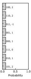
As a specific example, Fig. 4 shows a quantum circuit corresponding to the objective function $E(\mathbf{b})=1+b_{0}-1.8b_{1}b_{2}b_{3}$, where we set $n=4$ and $m=3$. Since we used the direct encoding method, $-1.8b_{1}b_{2}b_{3}$ was represented as $\mathbf{U}_{G}(-1.8\pi/4)$, and it was associated with three qubits $\Ket{b_{1}}$, $\Ket{b_{2}}$, and $\Ket{b_{3}}$. Additionally, Fig. 4 shows the output probabilities of Fig. 4, where only the top 16 states are shown for the sake of readability. As given in (8), the direct encoding method may not result in a unique integer. For example, the states $(0111,-1)$ and $(0111,-2)$ had positive probabilities in Fig. 4. The state of interest here is $\mathbf{b}=[0~{}1~{}1~{}1]$ and $E(\mathbf{b})=1-1.8=-0.8<0$. That is, before amplitude amplification, at $L=0$, integers close to the real value are observed, and after amplification, at $L>0$, the negative states are observed with high probabilities. As shown in Fig. 4(d), the states $(0111,-1)$ and $(0111,-2)$ were amplified as the number of Grover operators $L$ increased, while the wrong state $(0111,-2)$ was observed with a lower probability than $(0111,-1)$. Another wrong state $(1111,-1)$ was also observed with a low probability. This is the reason why the correction of the objective function value is required for real-valued GAS, as summarized in Algorithm 2.

In the literature, a quantum circuit has been evaluated by the numbers of qubits and gates and its depth, while a quantum algorithm has been evaluated by query complexity.

We consider a MIMO communication scenario with $N_{\mathrm{t}}$ transmit antennas and $N_{\mathrm{r}}$ receive antennas, as illustrated in Fig. 5. The input $n$-bit sequence $\mathbf{b}=[b_{0}~{}b_{1}~{}\cdots~{}b_{n-1}]\in\mathbb{B}^{n}$ is mapped to a symbol vector $\mathbf{s}=[s_{0}~{}s_{1}~{}\cdots~{}s_{N_{\mathrm{t}}-1}]\in{\mathbb{C}}^{N_{\mathrm{t}}\times 1}$, where $s_{t}$ for $0\leq t\leq N_{\mathrm{t}}-1$ denotes a Gray-coded data symbol specified in 5G NR [35]. We represent this bit-to-symbol mapper as $\mathbf{s}=M(\mathbf{b})=M(b_{0},\cdots,b_{n-1})$, which will be defined in detail in Section IV-B. The baseband received symbols $\mathbf{r}\in\mathbb{C}^{N_{\mathrm{r}}\times 1}$ is given by

where $\mathbf{H}_{\mathrm{c}}\in{\mathbb{C}}^{N_{\mathrm{r}}\times N_{\mathrm{t}}}$ denotes the channel matrix, and $\mathbf{v}\in{\mathbb{C}}^{N_{\mathrm{r}}\times 1}$ denotes the additive white Gaussian noise. Here, we assume the narrowband Rayleigh flat fading. That is, each element of $\mathbf{H}_{\mathrm{c}}$, $h_{ut}$, and each element of $\mathbf{v}$, $v_{u}$, follow the standard complex Gaussian distribution $\mathcal{CN}(0,1)$ for $0\leq u\leq N_{\mathrm{r}}-1$ and $0\leq t\leq N_{\mathrm{t}}-1$. The SNR is defined as $\gamma=1/\sigma^{2}$ because the symbol vector has the power constraint $\mathrm{E}\left[\|\mathbf{s}/\sqrt{N_{\mathrm{t}}}\|_{\mathrm{F}}^{2}\right]=\mathrm{E}\left[\sum_{t=0}^{N_{\mathrm{t}}-1}|s_{t}|^{2}/N_{\mathrm{t}}\right]=1$. The constellation size, or modulation order, is denoted by $L_{\mathrm{c}}$, and the transmission rate is calculated by

Corresponding to (10), the ideal MLD is performed as

where we have the objective function

From (12), the exhaustive search using a classical computer requires the computational time complexity of $O(2^{n})$, which is equivalent to the query complexity in CD. Both complexities increase exponentially with the transmission rate $n$.

To mitigate the exponential complexity, a number of low-complexity detectors have been proposed in the literature. The classic ZF detector uses the pseudo-inverse matrix of

and enables independent detection of data symbols as

where $M^{-1}\left(\cdot\right)$ denotes the hard-decision symbol-to-bit demapper. Similarly, the MMSE detector uses

and obtains

An MMSE-based interference cancelation method has been adopted in typical wireless standards such as 5G NR. The performance of a ZF or MMSE detector is worse than that of MLD. In general, low-complexity detectors improve complexity at the sacrifice of performance.

The above system model and detectors are typical and common in the field of wireless communications. Since we consider a general MIMO system, the simulation results given in this paper are the same as those for a multicarrier scenario without inter-subcarrier interference or an uplink multi-user scenario in which $N_{\mathrm{t}}$ single-antenna user terminals transmit their symbols and these symbols are received simultaneously at a base station equipped with $N_{\mathrm{r}}$ antennas.

As described in Section III, the proposed GAS is capable of solving a real-valued HUBO problem. We transform the objective function of MIMO MLD (13) into a HUBO problem. Specifically, we use the relationship between transmission bits and data symbols, which is specified in the 5G NR standard [35]. The input $n$-bit sequence is denoted by $\mathbf{b}=[b_{0}~{}b_{1}~{}\cdots~{}b_{n-1}]\in\mathbb{B}^{n}$ and the symbol vector is denoted by $\mathbf{s}=[s_{0}~{}s_{1}~{}\cdots~{}s_{N_{\mathrm{t}}-1}]\in\mathbb{C}^{N_{\mathrm{t}}}$. Then, BPSK symbols $\mathbf{s}=M_{2}(\mathbf{b})$ are generated by [35]

and QPSK symbols $\mathbf{s}=M_{4}(\mathbf{b})$ are generated by [35]

Furthermore, 16-QAM symbols $\mathbf{s}=M_{16}(\mathbf{b})$ are generated by [35]

and 64-QAM symbols $\mathbf{s}=M_{64}(\mathbf{b})$ are generated by [35]

A similar relationship for 256-QAM is defined in [35] and its extension for higher modulation orders can be defined easily.

Overall, Fig. 6 shows the Gray-coded data symbols defined by (18), (19), and (IV-B).

Our proposed objective function is obtained by substituting $M(\cdot)$ in (13) with (18), (19), (IV-B), or (IV-B), which contains $n$ number of binary variables $b_{0},\cdots,b_{n-1}$. In the cases of BPSK and QPSK, our objective function results in a quadratic form since both symbols are represented by a linear relationship and the MLD (12) contains the square of the Frobenius norm. In the case of 16-QAM, the objective function results in a quartic form since the symbols are represented by a quadratic relationship. Similarly, the objective function results in a sextic form in the 64-QAM case.

The use of data symbols specified in 5G NR is not straightforward since the objective function inevitably contains higher-order terms if the modulation order is 16 or higher. Thus, in this form, the conventional QA requires a transformation from HUBO to QUBO, and this transformation involves an increase in binary variables, making the problem more difficult. Our proposed approach is only possible with the aid of the real-valued support of GAS. Because of GAS, the query complexity is expected to be reduced from $O(2^{n})$ to $O(\sqrt{2^{n}})$.

The structure of the proposed objective function depends only on the number of transmit antennas, $N_{\mathrm{t}}$, the number of receive antennas, $N_{\mathrm{r}}$, and the modulation order, $L_{\mathrm{c}}$. The coefficients in the objective function change depending on the channel matrix $\mathbf{H}_{\mathrm{c}}$. The calculation cost of coefficients determines the complexity of classical processing required before executing GAS, which relates to the latency of the algorithm. If we approximate the computational complexity as the number of real-valued multiplications, the largest burden is the product of channel coefficients, such as $h_{00}h_{01}^{*}$. The total number of multiplications is calculated as $4N_{\mathrm{r}}N_{\mathrm{t}}(N_{\mathrm{t}}-1)/2=O(N_{\mathrm{r}}N_{\mathrm{t}}^{2})$, which is sufficiently small with respect to the detection complexity.

GAS obtains a global minimum solution by updating the threshold value $y_{i}$ and amplifying the probability amplitudes corresponding to values smaller than the threshold. The query complexity can be reduced by setting the initial threshold in a manner different from that in classic random sampling, although the asymptotic performance may not change. In this section, we derive the probability distribution of the objective function value and use it to determine a strict threshold, which enables further speedup.

If the information bits in (13) are estimated correctly, the minimum value of (13) is the Frobenius norm of additive noise $\mathbf{v}\in\mathbb{C}^{N_{\mathrm{r}}\times 1}$ as follows:

That is, $E_{\mathrm{min}}$ depends on the noise variance $\sigma^{2}$, which is typically known at the receiver, and instantaneous noise $v_{u}$, which is unknown in any case. Since the noise is assumed to follow the complex Gaussian distribution, the magnitude of the norm follows the Rayleigh distribution, and its square follows the exponential distribution. As a result, $E_{\mathrm{min}}$ in (24) follows the Erlang distribution, whose probability density function is

where we have SNR $\gamma=1/\sigma^{2}$. The corresponding cumulative distribution function (CDF) is given by

As an example, if we consider the case with $N_{\mathrm{r}}=2$, the CDF is calculated as

from (26). Fig. 8 exemplifies CDF (27) when SNR is varied as $\gamma=5$ to $20$ dB. Additionally, the CDF of the simulated objective function values with $N_{\mathrm{t}}=2$ and QPSK is also plotted. As shown in Fig. 8, if the SNR is sufficient, such as above 10 dB, the theoretical and simulated values are identical. Thus, it is possible to know in advance that the minimum value to be calculated is below a certain threshold, which can be determined with a very high degree of certainty. Given an SNR $\gamma$, theoretical values of (26) can be used to determine a strict threshold.

From (26), the probability that the threshold $y$ is below the minimum value is

Let $\tilde{y}$ be the threshold to be determined and $P$ be a small constant probability, such as $P=10^{-3}$ and $10^{-4}$. Replacing $y$ and $\mathrm{Pr}[Y>y]$ in (28) with $\tilde{y}$ and $P$ yields

Dividing both sides by $-e$ gives

Then, using the Lambert $W$ function, we obtain

where $W_{-1}(\cdot)$ denotes the lower branch of the Lambert $W$ function, i.e., $W_{-1}(\cdot)\leq-1$ and $W_{-1}(-1/e)=-1$. Finally, the threshold to be determined is

which is similar to (24), and

Here, $\nu$ is a positive constant and is calculated once before running our proposed algorithm. For example, we have $\nu=9.23$ if $P=10^{-3}$ and $\nu=11.8$ if $P=10^{-4}$.

For further speedup, we opt to use the output of the MMSE detector (16). In [13], Botsinis et al. proposed the MMSE-based threshold of

where we have a rough estimate $\bar{\mathbf{b}}_{0}=M^{-1}(\mathbf{W}_{\mathrm{MMSE}}\mathbf{r})$. Our proposed threshold $\tilde{y}$, which is simpler than $\bar{y}$, can be used together with $\bar{y}$. Specifically, we calculate both $\tilde{y}$ and $\bar{y}$ at the beginning of Algorithm 2, set the initial threshold as the smaller of the two, and initialize the first solution with $\bar{\mathbf{b}}_{0}$. Let $\mathbf{b}_{0}$ be a random $n$-bit sequence. The initial threshold used for the proposed Algorithm 2 can be summarized as follows:

One problem with the proposed threshold $\tilde{y}$ and the combination $\min(\bar{y},\tilde{y})$ is that they may become smaller than the actual minimum. In this case, since there are no states of interest, GAS will be in a state where the solution $\mathbf{b}_{i}$ in Algorithm 2 is not updated. The probability of this undesirable event occurring is $P$, i.e.,

because we have the relationship $\mathrm{Pr}[\bar{y}<E_{\mathrm{min}}]=0$. Then, it can be expected that the proposed threshold $\tilde{y}$ may degrade the bit error ratio (BER) significantly if $P$ is inappropriate. Specifically, the BER of the proposed threshold $\tilde{y}$ is approximated by

where $\mathrm{BER}_{\mathrm{MLD}}$ is the BER of MLD. In the proposed combination method, we initialize the first solution with the MMSE output $\bar{\mathbf{b}}_{0}$. Since the initial threshold $\min(\bar{y},\tilde{y})$ becomes smaller than the actual minimum with probability $P$, the BER of the proposed combination method is approximated by

where $\mathrm{BER}_{\mathrm{\mathrm{MMSE}}}$ is the BER of the MMSE detector. Both (37) and (38) indicate that the design of $P$ exerts no significant effect as long as it is smaller than $\mathrm{BER}_{\mathrm{MLD}}$, which can be calculated exactly in a closed form in advance. For our performance analysis, the effect of $P$ is shown in Fig. 13.

A quantum circuit for GAS is composed of $\mathbf{H}$, $\mathbf{X}$, $\mathbf{Z}$, phase, controlled-phase gates, and the IQFT. In particular, the state preparation operator $\mathbf{A}_{y_{i}}$ is the most complex part corresponding to the objective function and is dynamically configured in accordance with the threshold $y_{i}$. In the quantum circuit $\mathbf{A}_{y_{i}}$, the number of controlled-phase gates depends on the number of terms in the objective function. We therefore derive the number of terms in the objective function that correspond to each order in an algebraic manner. Ignoring the power scaling factor, the objective function of MIMO MLD (13) is transformed into

Here, we focus on three types of terms: first-order terms such as $-r^{*}_{0}h_{00}s_{0}$ and $-r_{0}h^{*}_{00}s^{*}_{0}$, squares of the same symbol such as $|h_{00}|^{2}|s_{0}|^{2}$ and $|h_{01}|^{2}|s_{1}|^{2}$, and products of two symbols such as $h_{00}h^{*}_{10}s_{0}s^{*}_{1}$ and $h^{*}_{00}h_{10}s^{*}_{0}{s}_{1}$.

For example, in the relatively simple QPSK case, squares of the same symbol result in constant terms because of (19). First-order terms directly result in first-order terms with respect to binary variables. Products between two symbols result in products of binary variables. If $N_{\mathrm{t}}=2$ and $N_{\mathrm{r}}=2$, four second-order terms appear: $b_{0}b_{2},b_{1}b_{3},b_{0}b_{3},$ and $b_{1}b_{2}$. The number of corresponding terms is equal to the combination of two choices from $N_{\mathrm{t}}$ antennas, e.g.,

where we have the relationship $n=N_{\mathrm{t}}\cdot\log_{2}(L_{\mathrm{c}})=2N_{\mathrm{t}}$. In total, the number of second-order terms is calculated as $4\cdot n(n-2)/8=n(n-2)/2$.

References

- [1] M. A. Nielsen and I. L. Chuang, Quantum Computation and Quantum Information, 10th ed. Cambridge ; New York: Cambridge University Press, 2010.
- [2] P. Shor, “Algorithms for quantum computation: Discrete logarithms and factoring,” in Proceedings 35th Annual Symposium on Foundations of Computer Science, Nov. 1994, pp. 124–134.
- [3] D. E. Knuth, “Big Omicron and big Omega and big Theta,” ACM SIGACT News, vol. 8, no. 2, pp. 18–24, 1976.
- [4] L. K. Grover, “A fast quantum mechanical algorithm for database search,” in Proceedings of the Twenty-Eighth Annual ACM Symposium on Theory of Computing. Philadelphia, Pennsylvania, United States: ACM Press, 1996, pp. 212–219.
- [5] D. Bulger, W. Baritompa, and G. Wood, “Implementing pure adaptive search with Grover’s quantum algorithm,” Journal of Optimization Theory and Applications, vol. 116, pp. 517–529, Mar. 2003.
- [6] C. Gidney, “Halving the cost of quantum addition,” Quantum, vol. 2, p. 74, 2018.
- [7] A. Gilliam, M. Pistoia, and C. Gonciulea, “Optimizing quantum search using a generalized version of Grover’s algorithm,” arXiv:2005.06468 [quant-ph], May 2020.
- [8] A. Gilliam, S. Woerner, and C. Gonciulea, “Grover adaptive search for constrained polynomial binary optimization,” Quantum, vol. 5, p. 428, Apr. 2021.
- [9] T. Kadowaki and H. Nishimori, “Quantum annealing in the transverse Ising model,” Phys. Rev. E, vol. 58, pp. 5355–5363, Nov 1998.
- [10] P. Botsinis, S. X. Ng, and L. Hanzo, “Quantum search algorithms, quantum wireless, and a low-complexity maximum likelihood iterative quantum multi-user detector design,” IEEE Access, vol. 1, pp. 94–122, 2013.
- [11] M. Boyer, G. Brassard, P. Høyer, and A. Tapp, “Tight bounds on quantum searching,” Fortschritte der Physik, vol. 46, no. 4-5, pp. 493–505, 1998.
- [12] C. Durr and P. Hoyer, “A quantum algorithm for finding the minimum,” arXiv:quant-ph/9607014, Jan. 1999.
- [13] P. Botsinis, S. X. Ng, and L. Hanzo, “Fixed-complexity quantum-assisted multi-user detection for CDMA and SDMA,” IEEE Transactions on Communications, vol. 62, no. 3, pp. 990–1000, Mar. 2014.
- [14] P. Botsinis, D. Alanis, S. X. Ng, and L. Hanzo, “Low-complexity soft-output quantum-assisted multiuser detection for direct-sequence spreading and slow subcarrier-hopping aided SDMA-OFDM systems,” IEEE Access, vol. 2, pp. 451–472, 2014.
- [15] P. Botsinis, D. Alanis, Z. Babar, S. X. Ng, and L. Hanzo, “Iterative quantum-assisted multi-user detection for multi-carrier interleave division multiple access systems,” IEEE Transactions on Communications, vol. 63, no. 10, pp. 3713–3727, Oct. 2015.
- [16] ——, “Noncoherent quantum multiple symbol differential detection for wireless systems,” IEEE Access, vol. 3, pp. 569–598, 2015.
- [17] W. Ye, W. Chen, X. Guo, C. Sun, and L. Hanzo, “Quantum search-aided multi-user detection for sparse code multiple access,” IEEE Access, vol. 7, pp. 52 804–52 817, 2019.
- [18] D. Alanis, P. Botsinis, Z. Babar, H. V. Nguyen, D. Chandra, S. X. Ng, and L. Hanzo, “A quantum-search-aided dynamic programming framework for pareto optimal routing in wireless multihop networks,” IEEE Transactions on Communications, vol. 66, no. 8, pp. 3485–3500, Aug. 2018.
- [19] ——, “Quantum-aided multi-objective routing optimization using back-tracing-aided dynamic programming,” IEEE Transactions on Vehicular Technology, vol. 67, no. 8, pp. 7856–7860, Aug. 2018.
- [20] P. Botsinis, D. Alanis, S. Feng, Z. Babar, H. V. Nguyen, D. Chandra, S. X. Ng, R. Zhang, and L. Hanzo, “Quantum-assisted indoor localization for uplink mm-wave and downlink visible light communication systems,” IEEE Access, vol. 5, pp. 23 327–23 351, 2017.
- [21] P. Botsinis, D. Alanis, Z. Babar, S. X. Ng, and L. Hanzo, “Coherent versus non-coherent quantum-assisted solutions in wireless systems,” IEEE Wireless Communications, vol. 24, no. 6, pp. 144–153, Dec. 2017.
- [22] P. Botsinis, D. Alanis, Z. Babar, H. V. Nguyen, D. Chandra, S. X. Ng, and L. Hanzo, “Quantum search algorithms for wireless communications,” IEEE Communications Surveys Tutorials, vol. 21, no. 2, pp. 1209–1242, 2019.
- [23] K. Fujii, “Noise threshold of quantum supremacy,” arXiv:1610.03632 [quant-ph], Oct. 2016.
- [24] C. Gidney and M. Ekerå, “How to factor 2048 bit RSA integers in 8 hours using 20 million noisy qubits,” Quantum, vol. 5, p. 433, Apr. 2021.
- [25] N. Ishikawa, “Quantum speedup for index modulation,” IEEE Access, vol. 9, pp. 111 114–111 124, 2021.
- [26] G. Jay, “IBM Quantum roadmap to build quantum-centric supercomputers,” https://research.ibm.com/blog/ibm-quantum-roadmap-2025, May 2022.
- [27] D. Stilck Franca and R. Garcia-Patron, “Limitations of optimization algorithms on noisy quantum devices,” Nature Physics, vol. 17, no. 11, pp. 1221–1227, 2021.
- [28] M. Kim, D. Venturelli, and K. Jamieson, “Leveraging quantum annealing for large MIMO processing in centralized radio access networks,” Proceedings of the ACM Special Interest Group on Data Communication, pp. 241–255, Aug. 2019.
- [29] S. Mondal, M. R. Laskar, and A. K. Dutta, “ML criterion based signal detection of a MIMO-OFDM system using quantum and semi-quantum assisted modified DHA/BBHT search algorithm,” IEEE Transactions on Vehicular Technology, vol. 70, no. 2, pp. 1688–1698, Feb. 2021.
- [30] Z. Babar, Z. B. Kaykac Egilmez, L. Xiang, D. Chandra, R. G. Maunder, S. X. Ng, and L. Hanzo, “Polar codes and their quantum-domain counterparts,” IEEE Communications Surveys Tutorials, vol. 22, no. 1, pp. 123–155, 2020.
- [31] T. Matsumine, T. Koike-Akino, and Y. Wang, “Channel decoding with quantum approximate optimization algorithm,” in IEEE International Symposium on Information Theory, Jul. 2019, pp. 2574–2578.
- [32] T. Ohyama, Y. Kawamoto, and N. Kato, “Intelligent reflecting surface (IRS) allocation scheduling method using combinatorial optimization by quantum computing,” IEEE Transactions on Emerging Topics in Computing, vol. 10, no. 3, 2022.
- [33] G. Brassard, P. Hoyer, and A. Tapp, “Quantum counting,” arXiv:quant-ph/9805082, vol. 1443, pp. 820–831, 1998.
- [34] G. Brassard, P. Hoyer, M. Mosca, and A. Tapp, “Quantum amplitude amplification and estimation,” arXiv:quant-ph/0005055, vol. 305, pp. 53–74, 2002.
- [35] 3GPP, “TS 138 211 - V15.2.0 - 5G; NR; Physical channels and modulation (3GPP TS 38.211 version 15.2.0 Release 15),” 2018.
- [36] A. Barenco, C. H. Bennett, R. Cleve, D. P. DiVincenzo, N. Margolus, P. Shor, T. Sleator, J. A. Smolin, and H. Weinfurter, “Elementary gates for quantum computation,” Physical Review A, vol. 52, no. 5, pp. 3457–3467, Nov. 1995.