Quantity vs. Quality: On Hyperparameter Optimization for Deep Reinforcement Learning
Abstract
Reinforcement learning algorithms can show strong variation in performance between training runs with different random seeds. In this paper we explore how this affects hyperparameter optimization when the goal is to find hyperparameter settings that perform well across random seeds. In particular, we benchmark whether it is better to explore a large quantity of hyperparameter settings via pruning of bad performers, or if it is better to aim for quality of collected results by using repetitions. For this we consider the Successive Halving, Random Search, and Bayesian Optimization algorithms, the latter two with and without repetitions. We apply these to tuning the PPO2 algorithm (Schulman et al., 2017) on the Cartpole balancing task and the Inverted Pendulum Swing-up task. We demonstrate that pruning may negatively affect the optimization and that repeated sampling does not help in finding hyperparameter settings that perform better across random seeds. From our experiments we conclude that Bayesian optimization with a noise robust acquisition function is the best choice for hyperparameter optimization in reinforcement learning tasks.
1 Introduction
Many reinforcement learning methods can show significant variation in performance between runs with different random seeds (Henderson et al., 2018; Islam et al., 2017; Nagarajan et al., 2018; Colas et al., 2018). This poses an issue for conducting hyperparameter optimization where the goal is to find hyperparameters configurations that perform well across random seeds.
Common hyperparameter optimization strategies typically assume exact observations or a negligible amount of uncertainty. For example, most hyperparameter optimization algorithms check different settings and then suggest the best observed. However, if observations vary drastically between random seeds, the best observed configuration may not be the configuration that performs best when averaged across many random seeds. Most model-free hyperparameter optimization methods such as random search (Bergstra and Bengio, 2012), successive halving (Jamieson and Talwalkar, 2016; Li et al., 2016), and population-based training (Jaderberg et al., 2017) do not explicitly handle uncertainty in observations. Evolutionary algorithms can in fact handle uncertainty (Loshchilov and Hutter, 2016). However, these methods may require more observations than is often feasible for hyperparameter optimization. Finally, model-based methods such as Bayesian optimization have a principled way to model uncertainty. However, they depend on an acquisition function to decide on the next query point (Picheny et al., 2013). Not all acquisition functions are robust to uncertainty in the observations and especially the most commonly expected improvement is not.
In order to deal with uncertainty in hyperparameter optimization, some researchers have adopted the practice of averaging across random seeds even during the hyperparameter search itself (Balandat et al., 2019; Falkner et al., 2018; Duan et al., 2016). Other sources (Hill et al., 2018) use hyperparameter optimization algorithms that are known to generally perform well but do not handle uncertainty. In this paper we assume that the goal is to find a hyperparameter optimization that performs well across random seeds. With that in mind, we benchmark different hyperparameter optimization strategies tuning a deep reinforcement learning algorithm on two continuous control tasks.
2 Methods
2.1 Problem Statement
In order to define the problem we consider hyperparameters . We define the mean reward resulting from training with and a randomly picked seed as . Finally, we define the expected mean reward across all random seeds for that hyperparameter settings as . The goal of the hyperparameter optimization here is to find
| (1) |
that is the hyperparameter setting that yields the largest mean reward across random seeds. The optimization in equation 1 is difficult because is unavailable and observations are computationally expensive. In particular, hyperparameter optimization faces two problems:
-
1.
Choosing where to evaluate the next during the optimization may be impacted by uncertainty, because previous observations are not exact.
-
2.
Choosing at the end of the optimization may be impacted, because the true performance of each is uncertain.
2.2 Repeated Evaluation
A simple way to approximate is to collect repeated evaluations and average the measurements . While this approach is conceptually easy, the number of repetitions is often constrained by a computational budget. For this reason, the question is whether repetition is the optimal strategy or if it would be better to just evaluate more hyperparameter settings . We now review a number of commonly used approaches to hyperparameter optimization and how these approaches are impacted by uncertainty.
2.3 Model-free Optimization
Random Search
Random search is a simple and popular model-free hyperparameter search algorithm (Bergstra and Bengio, 2012). In particular, random search can often serve as a simple but robust baseline against more complex methods (Li and Talwalkar, 2019). In random search hyperparameter configurations are sampled uniformly at random from the specified hyperparameter space . At the end of the optimization, the best observed hyperparameter setting is picked.
When applying random search in a setting where there is uncertainty, the suggestion of hyperparameter configurations is not impacted. However, the choice of the final recommended configuration may be influenced. In the presence of uncertainty the best observed setting may not be the on-average best setting. This issue can be alleviated using repetition as described in Section 2.2, however at a higher computational cost. In experiments we denote random search as Random Search, Random Search x3, and Random Search x5 for using one, three, or five evaluations, respectively.
Bandit Algorithms
Another more recent approach to hyperparameter search is the bandit-based Successive Halving Algorithm (SHA) (Jamieson and Talwalkar, 2016), as well as its extensions Hyperband (Li et al., 2016), and Asynchronous Successive Halving (ASHA) (Li et al., 2018). SHA and Hyperband have been shown to outperform random search and state-of-the-art model-based search methods on many hyperparameter optimization benchmarks from the domain of supervised learning. SHA operates by randomly sampling configurations and allocating increasingly larger budgets to well-performing configurations. In the beginning, a small budget is allocated to each configuration. All configurations are evaluated and the top of configurations are promoted. Then the budget for each promoted configuration is increased by a factor of . This is repeated until the maximum per-configuration budget is reached. When tuning neural networks with SHA, the budget is usually the number of training iterations. That way the algorithm can probe a lot of configurations without fully evaluating them. An algorithm that closely resembles SHA is used to tune hyperparameters of deep reinforcement learning algorithms in the Stable-baselines (Hill et al., 2018) package. We imitate the setup there by using the number of training steps as the resource. We refer to this as ASHA in experiments since we are using the asynchronous version of SHA.
Evolutionary Algorithms
Lastly, evolutionary algorithms have recently been successfully applied to hyperparameter optimization and architecture search and hyperparameter optimization for neural networks (Real et al., 2017; Loshchilov and Hutter, 2016; Hansen et al., 2019). Evolutionary algorithms such as CMA-ES (Hansen et al., 2003) can handle high-dimensional search spaces and actually have a principled way of handling uncertainty. Nevertheless, evolutionary algorithms tend to require a larger number of function evaluations that is out of the scope of this study and may also be infeasible for many practitioners. For this reason, we leave the comparison to evolutionary algorithms for future work.
One algorithm from this paradigm that is popular with practitioners is Population-Based Training (PBT) (Jaderberg et al., 2017). In PBT a population of models is trained jointly with optimizing their hyperparameters. Contrary to most other hyperparameter optimization approaches, PBT finds schedules of hyperparameters via perturbation and replacement between generations. PBT has shown strong results in multiple domains including the training of reinforcement learning agents. The crucial difference in the goal of PBT and the goal we are aiming for in this paper is that PBT delivers one optimally trained agent. In this paper we however aim to obtain an optimal hyperparameter setting. While it is possible to trace back the schedule of hyperparameters of the best agent in PBT, we believe that it is less common to share and reproduce these. In addition, due to the fact that PBT finds schedules instead of specific hyperparameter settings it is difficult to accurately compare it to standard hyperparameter optimization methods which find fixed hyperparameters. For these reasons we do not include PBT in the experiments in Section 3.
2.4 Bayesian Optimization
(Bergstra et al., 2011) and (Snoek et al., 2012) demonstrated the feasibility of using Bayesian optimization for hyperparameter optimization. Bayesian optimization (BO) is a model-based approach to global derivative-free optimization of blackbox functions. Given existing observations of configurations and associated objective values, BO fits a surrogate model from the search space to the objective. This model is usually faster to evaluate than the objective function itself. For this reason, a large number of predictions of objective values can be made. An acquisition function describes the utility of each prediction. By maximizing the acquisition function one can find the optimal next point to evaluate.
As described by (Srinivas et al., 2009), it is common to use a Gaussian Process (GP) as a surrogate model for . For the covariance kernel the Matern 5/2 kernel is a common choice. Assuming normal observations noise, this offers a natural framework for uncertainty in observations. Inference for the observation variance can be made via maximization of the marginal likelihood. In particular, given a collection of observations and a GP prior, one can obtain the posterior distribution at hyperparameter setting as . Assuming a zero prior, the posterior mean and variance are given by:
where is the vector of covariances with all previous observations and is the covariance matrix of the observations.
Expected Improvement
As mentioned before, Bayesian optimization chooses the next point to evaluate via the acquisition function. The most popular choice of acquisition function for hyperparameter optimization is the expected improvement (EI) (Mockus et al., 1978). The EI is given by
| (2) |
where and is the minimum observed validation loss. Part of why the EI is popular is that it can be computed analytically. However, if observations are uncertain may be large and may just be low by chance. This can result in over-exploitation around and the optimization getting "stuck" around this point. In experiments we refer to EI as GPyOpt-EI since we are using the GPyOpt (authors, 2016) implementation. We also show experiments for GPyOpt-EI x3, referring to EI with averaging across three repetitions for each hyperparameter setting.
Noisy Expected Improvement
(Letham et al., 2019) extended expected improvement to handle uncertainty in observations by taking the expectation over observations. Ignoring constraint handling also introduced by the authors, the noisy expected improvement (NEI) can be written as:
| (3) |
where is a fantasy dataset sampled from the posterior and is the minimum of the fantasy dataset. In practice, this approach fits a GP model. GP samples are drawn from the posterior at the observed points. These samples represent fantasy datasets. Each fantasy dataset is treated as in the regular EI, that is, a GP is fitted and the EI is computed across the space . The EI values are then averaged across the fantasy datasets to obtain the NEI. Balandat et al. (2019) simplify this approach by taking the expectation over the joint posterior:
| (4) |
We note that Equation 3 and 4 are both computationally intensive and non-trivial to implement. However, Letham et al. (2019) showed that NEI outperforms regular EI on objective functions with Gaussian noise and given the true variance. In our experiments we use the qNEI implemented in BoTorch111https://botorch.org/ to calculate the noisy expected improvement. Contrary to the experiments in (Letham et al., 2019) we infer the variance . We refer to this approach as BoTorch-qNEI.
Lower Confidence Bound
An alternative to the EI criterion is the Lower(/Upper) Confidence Bound (LCB) criterion (Srinivas et al., 2009). The LCB takes the form
| (5) |
where is a coefficient set by the user. This coefficient is sometimes termed the exploration weight. Tuning the exploration weight may improve the performance of LCB. However, since in practice the computational budget to tune this parameter is rarely available, we use a default value of . While LCB has been shown to be outperformed by EI on noise-less objective functions (Snoek et al., 2012), contrary to EI it is not impacted by uncertainty in the observations. This is due to the fact that it only depends on the posterior mean and variance. In all experiments we refer to LCB as GPyOpt-LCB.
We note that there are more available acquisition functions than the ones presented in this section. In particular, the knowledge gradient (Scott et al., 2011; Wu and Frazier, 2016) is an acquisition function that, while difficult to compute, can handle uncertainty and has been shown to outperform the presented acquisition functions (Balandat et al., 2019). Furthermore, entropy-search-based methods (Hennig and Schuler, 2012; Hernández-Lobato et al., 2014; Wang and Jegelka, 2017) also naturally handle uncertainty. We leave the evaluation of these methods to future work.
While the choice of acquisition function determines how to choose the next point, one still needs to pick a best setting at the end of the optimization. In the noise-less case this is often done by picking the best observed hyperparameter . Frazier (2018) suggested to rely on the GP model and pick the best predicted . Since this approach is robust to uncertainty we use the predicted best in all experiments. To make this feasible in multi-dimensional tasks we find the best predicted by optimizing an LCB acquisition with , thereby utilizing existing optimization tools in BoTorch and GPyOpt.
3 Experiments
3.1 Cartpole Balancing
First, we compare the introduced algorithms on the cartpole balancing task. The cartpole task (Barto et al., 1983) is a continuous control problem that requires to balance a pole on a friction-less cart. The cart can be moved left or right. A screenshot of the task is shown in Figure 1.

The cartpole task has been used as a benchmark for reinforcement learning (RL) algorithms (Duan et al., 2016) and most recently to benchmark hyperparameter optimization for reinforcement learning (Falkner et al., 2018; Balandat et al., 2019). We tune the hyperparameters of the proximal policy optimization algorithm by Schulman et al. (2017). For this we use the implementation from Stable-baselines (Hill et al., 2018) and the Cartpole-v1 environment from OpenAI Gym (Brockman et al., 2016). In particular, we optimize the log-learning-rate (uniform ) as well as the entropy-coefficient (uniform ), discount-factor (uniform ), and likelihood-ratio-clipping (uniform ). The RL agent is trained for 30000 steps and we use the mean reward across training as the objective for the hyperparameter optimization.

The hyperparameter optimization itself is allowed to train 100 agents. This translates to 100 hyperparameter settings for methods without repetition and for example 20 hyperparameter settings if five repetitions per setting were used. After the budget is used up, the best configuration is trained 20 times with different random seeds and the mean across those runs is taken as the hyperparameter optimization outcome. Figure 2 (right) shows results for 40 hyperparameter optimization runs conducted in this fashion. Evaluation is also done after 25 and 50 agents have been trained (Figure 2 left and middle, respectively). Corresponding means are shown Table 1.
| Evaluations | 25 | 50 | 100 |
|---|---|---|---|
| ASHA | 125.2 | 135.0 | 134.4 |
| BoTorch-qNEI | 149.7 | 155.2 | 158.3 |
| GPyOpt-EI | 136.5 | 143.6 | 148.5 |
| GPyOpt-EI x3 | 93.7 | 133.5 | 151.9 |
| GPyOpt-LCB | 141.1 | 149.7 | 148.7 |
| Random Search | 112.0 | 130.3 | 139.1 |
| Random Search x3 | 85.6 | 102.6 | 123.0 |
| Random Search x5 | 69.6 | 89.1 | 105.7 |
From Figure 2 and Table 1 it can be seen that BoTorch-qNEI has the best results across all budgets, however the difference to other Bayesian optimization methods is small. GPyOpt-EI x3 performs worse in the beginning, but later catches up. This suggests that its three repetitions do not help in this case and would be better used to explore additional hyperparameter settings. ASHA seems to have some very good runs, but stagnates at a slightly worse performance than the Bayesian optimization methods. Random Search performs almost on-par with the Bayesian optimization methods after 100 evaluations. Random Search x3 and Random Search x5 perform worst overall, but do show steady improvement. In this case more evaluations may be needed for these methods to perform better.
3.2 Inverted Pendulum Swing-up
As a second experiment, we consider the Inverted Pendulum Swing-up task. Just like the Cartpole balancing task from Section 3.1, the Inverted Pendulum Swing-up task is a classic control problem. A screenshot of the environment is shown in Figure 3. The friction-less pendulum (red) starts in a random position with random velocity and the goal is to keep it standing up. To achieve this the agent can apply negative or positive effort to the joint. The reward is a function of how upright and still the pendulum is.

In comparison to the Cartpole balancing task, this problem is considered more difficult. We again apply the proximal policy algorithm by (Schulman et al., 2017). This time the hyperparameter search-space consists of the log-learning-rate (uniform ) and the log-entropy-coefficient (uniform ). The agent is given timesteps for training. The hyperparameter optimization objective is, as before, the mean reward across training.
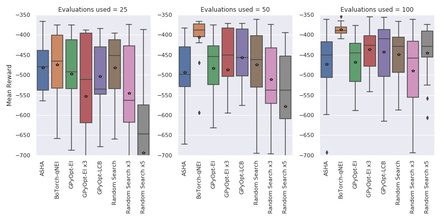
Figure 4 shows boxplots of mean rewards across training over 15 hyperparameter optimization runs. The hyperparameter optimization is again allowed to train 100 agents. Additional evaluations are again done after 25 and 50 trained agents. It can be seen that after 25 evaluations all algorithms perform similarly except for Random Search x5 which performs worse. After 50 evaluations BoTorch-qNEI clearly performs better than all other algorithms. This trend continues after 100 evaluations and except for BoTorch-qNEI no clear difference can be seen in the performance of the different algorithms. In terms of the median GPyOpt-LCB still performs second-best, however the distribution of its outcomes is very overlapping with that of the other methods. Table 2 shows corresponding means, nevertheless we believe that it is important to consider the distribution of outcomes for each method and believe Figure 4 better represents the results of this study.
| Evaluations | 25 | 50 | 100 |
|---|---|---|---|
| ASHA | -482.0 | -493.7 | -472.6 |
| BoTorch-qNEI | -474.7 | -406.2 | -387.3 |
| GPyOpt-EI | -497.2 | -483.5 | -467.5 |
| GPyOpt-EI x3 | -553.1 | -487.6 | -436.9 |
| GPyOpt-LCB | -503.7 | -456.2 | -442.4 |
| Random Search | -481.8 | -474.2 | -449.3 |
| Random Search x3 | -546.1 | -511.4 | -490.2 |
| Random Search x5 | -694.0 | -578.2 | -444.6 |
4 Discussion
We evaluated different hyperparameter optimization methods on two reinforcement learning benchmarks with the goal of finding hyperparameter settings that perform well across random seeds. The recorded outcome of each hyperparameter optimization is therefore the mean reward of the best setting averaged across multiple random seeds. From comparing algorithms on two reinforcement learning tasks we have found that model-based search in the form of GP-based Bayesian optimization performs best in terms of the average achieved across optimization runs. While in the Cartpole experiment all Bayesian optimization methods perform similarly, in the Inverted Pendulum the noise-robust expected improvement clearly outperforms other methods.
We find that, contrary to experiments from supervised learning, evaluating more configurations by using pruning as in the Successive Halving algorithm does not outperform Bayesian optimization in this case.
Furthermore, using replicates for each hyperparameter setting, as often done for reinforcement learning, does not outperform regular methods. For example, random search with one sample outperforms random search with three or five repetitions in both experiments when computation is matched. Using replication for Bayesian optimization does also not seem to improve performance.
5 Future Work
Future work on this topic include the evaluation of model-based multi-fidelity optimization such as introduced by (Poloczek et al., 2017) or (Wu et al., 2019). The question is whether such methods are better able to delineate noise even for partial evaluations of hyperparameter settings. Another direction for future work is to better model the observations of the objective, specifically with regards to the noise distribution. As mentioned before, NEI depends on the assumption of Gaussian noise and its performance may deteriorate if the observation noise is significantly non-Gaussian.
References
References
- authors [2016] The GPyOpt authors. GPyOpt: A bayesian optimization framework in python. http://github.com/SheffieldML/GPyOpt, 2016.
- Balandat et al. [2019] Maximilian Balandat, Brian Karrer, Daniel R Jiang, Samuel Daulton, Benjamin Letham, Andrew Gordon Wilson, and Eytan Bakshy. Botorch: Programmable bayesian optimization in pytorch. arXiv preprint arXiv:1910.06403, 2019.
- Barto et al. [1983] Andrew G Barto, Richard S Sutton, and Charles W Anderson. Neuronlike adaptive elements that can solve difficult learning control problems. IEEE transactions on systems, man, and cybernetics, (5):834–846, 1983.
- Bergstra and Bengio [2012] James Bergstra and Yoshua Bengio. Random search for hyper-parameter optimization. Journal of Machine Learning Research, 13(Feb):281–305, 2012.
- Bergstra et al. [2011] James S Bergstra, Rémi Bardenet, Yoshua Bengio, and Balázs Kégl. Algorithms for hyper-parameter optimization. In Advances in neural information processing systems, pages 2546–2554, 2011.
- Brockman et al. [2016] Greg Brockman, Vicki Cheung, Ludwig Pettersson, Jonas Schneider, John Schulman, Jie Tang, and Wojciech Zaremba. Openai gym. arXiv preprint arXiv:1606.01540, 2016.
- Colas et al. [2018] Cédric Colas, Olivier Sigaud, and Pierre-Yves Oudeyer. How many random seeds? statistical power analysis in deep reinforcement learning experiments. arXiv preprint arXiv:1806.08295, 2018.
- Duan et al. [2016] Yan Duan, Xi Chen, Rein Houthooft, John Schulman, and Pieter Abbeel. Benchmarking deep reinforcement learning for continuous control. In International Conference on Machine Learning, pages 1329–1338, 2016.
- Falkner et al. [2018] Stefan Falkner, Aaron Klein, and Frank Hutter. Bohb: Robust and efficient hyperparameter optimization at scale. arXiv preprint arXiv:1807.01774, 2018.
- Frazier [2018] Peter I Frazier. A tutorial on bayesian optimization. arXiv preprint arXiv:1807.02811, 2018.
- Hansen et al. [2003] Nikolaus Hansen, Sibylle D Müller, and Petros Koumoutsakos. Reducing the time complexity of the derandomized evolution strategy with covariance matrix adaptation (cma-es). Evolutionary computation, 11(1):1–18, 2003.
- Hansen et al. [2019] Nikolaus Hansen, Youhei Akimoto, and Petr Baudis. CMA-ES/pycma on Github. Zenodo, DOI:10.5281/zenodo.2559634, February 2019. URL https://doi.org/10.5281/zenodo.2559634.
- Henderson et al. [2018] Peter Henderson, Riashat Islam, Philip Bachman, Joelle Pineau, Doina Precup, and David Meger. Deep reinforcement learning that matters. In Thirty-Second AAAI Conference on Artificial Intelligence, 2018.
- Hennig and Schuler [2012] Philipp Hennig and Christian J Schuler. Entropy search for information-efficient global optimization. Journal of Machine Learning Research, 13(Jun):1809–1837, 2012.
- Hernández-Lobato et al. [2014] José Miguel Hernández-Lobato, Matthew W Hoffman, and Zoubin Ghahramani. Predictive entropy search for efficient global optimization of black-box functions. In Advances in neural information processing systems, pages 918–926, 2014.
- Hill et al. [2018] Ashley Hill, Antonin Raffin, Maximilian Ernestus, Adam Gleave, Anssi Kanervisto, Rene Traore, Prafulla Dhariwal, Christopher Hesse, Oleg Klimov, Alex Nichol, Matthias Plappert, Alec Radford, John Schulman, Szymon Sidor, and Yuhuai Wu. Stable baselines. https://github.com/hill-a/stable-baselines, 2018.
- Islam et al. [2017] Riashat Islam, Peter Henderson, Maziar Gomrokchi, and Doina Precup. Reproducibility of benchmarked deep reinforcement learning tasks for continuous control. arXiv preprint arXiv:1708.04133, 2017.
- Jaderberg et al. [2017] Max Jaderberg, Valentin Dalibard, Simon Osindero, Wojciech M Czarnecki, Jeff Donahue, Ali Razavi, Oriol Vinyals, Tim Green, Iain Dunning, Karen Simonyan, et al. Population based training of neural networks. arXiv preprint arXiv:1711.09846, 2017.
- Jamieson and Talwalkar [2016] Kevin Jamieson and Ameet Talwalkar. Non-stochastic best arm identification and hyperparameter optimization. In Artificial Intelligence and Statistics, pages 240–248, 2016.
- Letham et al. [2019] Benjamin Letham, Brian Karrer, Guilherme Ottoni, Eytan Bakshy, et al. Constrained bayesian optimization with noisy experiments. Bayesian Analysis, 14(2):495–519, 2019.
- Li and Talwalkar [2019] Liam Li and Ameet Talwalkar. Random search and reproducibility for neural architecture search. arXiv preprint arXiv:1902.07638, 2019.
- Li et al. [2018] Liam Li, Kevin Jamieson, Afshin Rostamizadeh, Ekaterina Gonina, Moritz Hardt, Benjamin Recht, and Ameet Talwalkar. Massively parallel hyperparameter tuning. arXiv preprint arXiv:1810.05934, 2018.
- Li et al. [2016] Lisha Li, Kevin Jamieson, Giulia DeSalvo, Afshin Rostamizadeh, and Ameet Talwalkar. Hyperband: A novel bandit-based approach to hyperparameter optimization. arXiv preprint arXiv:1603.06560, 18(1):6765–6816, 2016.
- Loshchilov and Hutter [2016] Ilya Loshchilov and Frank Hutter. Cma-es for hyperparameter optimization of deep neural networks. arXiv preprint arXiv:1604.07269, 2016.
- Mockus et al. [1978] Jonas Mockus, Vytautas Tiesis, and Antanas Zilinskas. The application of bayesian methods for seeking the extremum. Towards global optimization, 2(117-129):2, 1978.
- Nagarajan et al. [2018] Prabhat Nagarajan, Garrett Warnell, and Peter Stone. The impact of nondeterminism on reproducibility in deep reinforcement learning. 2018.
- Picheny et al. [2013] Victor Picheny, Tobias Wagner, and David Ginsbourger. A benchmark of kriging-based infill criteria for noisy optimization. Structural and Multidisciplinary Optimization, 48(3):607–626, 2013.
- Poloczek et al. [2017] Matthias Poloczek, Jialei Wang, and Peter Frazier. Multi-information source optimization. In Advances in Neural Information Processing Systems, pages 4288–4298, 2017.
- Real et al. [2017] Esteban Real, Sherry Moore, Andrew Selle, Saurabh Saxena, Yutaka Leon Suematsu, Jie Tan, Quoc V Le, and Alexey Kurakin. Large-scale evolution of image classifiers. In Proceedings of the 34th International Conference on Machine Learning-Volume 70, pages 2902–2911. JMLR. org, 2017.
- Schulman et al. [2017] John Schulman, Filip Wolski, Prafulla Dhariwal, Alec Radford, and Oleg Klimov. Proximal policy optimization algorithms. arXiv preprint arXiv:1707.06347, 2017.
- Scott et al. [2011] Warren Scott, Peter Frazier, and Warren Powell. The correlated knowledge gradient for simulation optimization of continuous parameters using gaussian process regression. SIAM Journal on Optimization, 21(3):996–1026, 2011.
- Snoek et al. [2012] Jasper Snoek, Hugo Larochelle, and Ryan P Adams. Practical bayesian optimization of machine learning algorithms. In Advances in neural information processing systems, pages 2951–2959, 2012.
- Srinivas et al. [2009] Niranjan Srinivas, Andreas Krause, Sham M Kakade, and Matthias Seeger. Gaussian process optimization in the bandit setting: No regret and experimental design. arXiv preprint arXiv:0912.3995, 2009.
- Wang and Jegelka [2017] Zi Wang and Stefanie Jegelka. Max-value entropy search for efficient bayesian optimization. In Proceedings of the 34th International Conference on Machine Learning-Volume 70, pages 3627–3635. JMLR. org, 2017.
- Wu and Frazier [2016] Jian Wu and Peter Frazier. The parallel knowledge gradient method for batch bayesian optimization. In Advances in Neural Information Processing Systems, pages 3126–3134, 2016.
- Wu et al. [2019] Jian Wu, Saul Toscano-Palmerin, Peter I Frazier, and Andrew Gordon Wilson. Practical multi-fidelity bayesian optimization for hyperparameter tuning. arXiv preprint arXiv:1903.04703, 2019.