Quadrupole dominance in the light Sn and in the Cd isotopes
Abstract
- Background
-
The of the Sn isotopes for exhibit enhancements hitherto unexplained. The same is true for all the Cd isotopes.
- Purpose
-
To describe the electromagnetic properties of the Sn and Cd isotopes.
- Method
-
Shell-model calculations are performed with a minimally renormalized realistic interaction, supplemented by quasi- and pseudo-SU3 symmetries and Nilsson-SU3 self-consistent calculations. Special care is devoted to the monopole part of the Hamiltonian.
- Results
-
(1) Shell-model calculations with the neutron effective charge as single free parameter describe well the and rates for in the Cd and Sn isotopes. The former exhibit weak permanent deformation corroborating the prediction of a pseudo-SU3 symmetry, which remains of heuristic value in the latter, where the pairing force erodes the quadrupole dominance. Calculations in - and -dimensional spaces exhibit almost identical behavior: A vindication of the shell model. (2) Nilsson-SU3 calculations describe patterns in 112-120Cd and 116-118Sn isotopes having sizable quadrupole moment of non-rotational origin denoted as q-vibrations.
- Conclusion
-
A radical reexamination of traditional interpretations in the region has been shown to be necessary, in which approximate symmetries involving the quadrupole force and a high quality monopole Hamiltonian play a major role. What emerges is a bumpy but coherent view.
I Introduction
All nuclear species are equal, but some are more equal than others. The tin isotopes deserve pride of place, because is the most resilient of the magic numbers, because they are very numerous, and many of them stable, starting at . For these, accurate data have been available for a long time. As seen in Fig. 1, a parabola accounts very well for their trend, except at 112-114Sn.

That these early results (Jonsson et al. [2]) truly signaled a change of regime became evident through work on the unstable isomers, starting with the measurement in 108Sn by Banu et al. [3]. A flurry of activity followed [4, 5, 6, 7, 8, 9, 10], from which a new trend emerged in which the parabola, characteristic of a seniority scheme, gives way to a platform, predicted by a pseudo-SU3 scheme (the squares). Here, I am going a bit fast, to follow the injunction of Montaigne: start by the last point (“Je veux qu’on comance par le dernier point” Essais II 10) [11, p. 296]. To slow down, I note that the idea to associate the plateau with pseudo-SU3, originated in a study of the cadmium isotopes, where quadrupole dominance is stronger and its consequences more clear-cut. Therefore, it is convenient to study the Cd and Sn families together. Section II provides the necessary tools.
II Theoretical framework
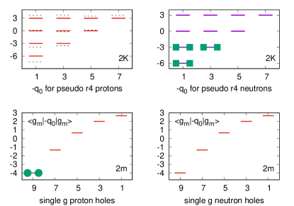
The basic idea is inspired by Elliott’s SU3 scheme [12, 13] and consists in building intrinsic determinantal states that maximize , the expectation value of the quadrupole operator , i.e., = [14, 15, 16]. Fig. 2 implements the idea for 104Cd (). The single-shell contribution (S) of the proton orbit (S) is given by Eq.(1) (with changed sign for hole states) with being the first unfilled orbit for prolate deformation. For the neutron orbits, the pseudo-SU3 scheme [17, 18, 16] (P generically, P for specific cases) amounts to assimilating all the orbits of a major osillator shell of principal quantum number , except the largest (the set) into orbits of the major shell. In our case the shell has , and is assimilated into a shell. As the operator is diagonal in the oscillator quanta representation, maximum is obtained by orderly filling states , with = 6, 3, 3, 0, 0…-3, -3, as in Fig. 2. Using for the cumulated value (e.g. 24 for 104Cd in Fig. 2), the intrinsic quadrupole moment then follows as a sum of the single-shell (S) and pseudo-SU3 (P) contributions
| (1) | |||
| (2) |
where I have introduced effective charges and recovered dimensions through with and . To adapt Eq. (2) to Sn, simply drop the S part (i.e., the term).
| 100 | 102 | 104 | 106 | 108 | 110 | |
| 2 | 4 | 6 | 8 | 10 | 12 | |
| 12 | 18 | 24 | 24 | 24 | 24 | |
| 14.8 | 21.6 | 29.5 | 30.0 | 29.6 | 29.3 | |
| B20e | 560(4) | 562(46)) | 779(80) | 814(24) | 838(28) | 852(42) |
| B20sp | 327 | 536 | 799 | 808 | 817 | 825 |
| B20SP | 317 | 511 | 795 | 824 | 817 | 813 |
To qualify as a Bohr Mottelson rotor, must coincide with the intrisic spectroscopic and transition quadrupole moments, defined through (as, e.g, in Ref. [16])
| (3) |
| (4) | |||
| (5) |
To speak of deformed nuclei two conditions must be met: =1.43 (the Alaga rule from Eq. (4)), and the “quadrupole quotient” rule, which follows from Eqs.(3) and (4) by equating (for ):
| (6) |
Full verification demands calculations but Eq. (5) can be checked directly by inspecting Fig. 2 as done in Table 1, that will be analyzed once the shell-model results are in.
These results rely on diagonalizations in spaces defined by , for Cd and 10 for Sn. The proton () and neutron () excitations are restricted to have . The calculations were done for (the case in Fig. 2), 111, 101 and 202 using variants [21] of the precision interaction N3LO [22] (denoted as I in what follows) with oscillator parameter = 8.4 MeV and cutoff fm-1. As a first step the monopole part of I is removed and replaced by single-particle energies for 100Sn from Ref. [23] referred to as GEMO for general monopole: a successful description of particle and hole spectra on magic nuclei from O to Pb, in particular consistent with the analysis of Ref. [24] for 100 Sn. Specifically 0.0, 0.5, 0.8 and 1.6 MeV. for 5/2, 7/2, 1/2, and 3/2, respectively.)
The I interaction is then renormalized by increasing the quadrupole and pairing components by q10% and p10%, respectively, and subject to an overall 1.1 scaling to account for renormalizations of other origins. The resulting interactions are called I.q.p. According to Ref. [25], the quadrupole renormalization (due to 2perturbative couplings) amounts to 30%, a theoretically sound result, empirically validated by the best phenomenological interactions in the and shells. By the same token the effective charges in 0spaces are estimated as = (0.46, 1.31), as confirmed in Refs. [26, 27]. For the pairing component, perturbation theory is not a good guide, but comparison with the phenomenological interactions demands a 40% increase [25, 15]. It follows that I.3.4 and = (0.46, 1.31) should be taken as standard for full 0spaces.
As I will be working in very truncated bases, which demand large effective charges, renormalizations should be implemented to account for polarization mechanisms that involve excitations to the shell. Proton jumps will contribute to and are expected to have greater impact than the corresponding neutron jumps, rapidly blocked by the particles. As a consequence, I set , a guess close to the standard value, and let vary, thus becoming the only adjustable parameter in the calculations, a choice validated later in Sec. V.
III The light Cd isotopes
In Fig. 3 it is seen that and 101 give the same results provided is properly chosen. There is little difference between and because as soon as neutrons are added they block the corresponding jumps, as mentioned above.

The calculation exhibits near perfect agreement with the Alaga rule:( ). In the figure it is shown for but it holds as well for 000 and 111. The more stringent quadrupole quotient rule Eq. (6) yields an average for 106-110Cd, corroborating the existence of a deformed region. As announced immediately after Eq. (6), Eq. (5) can be checked directly by inspecting Fig. 2, as done in Table 1 describing the “back of an envelope” SP estimates. Note that the naive form of P used so far (in and B20sp) is supplemented by the more accurate and B20SP using fully diagonalized values of . The remarkable property of the space that produces four identical values for has already been put to good use in Ref. [14] and Ref. [15, Fig. 38, TableVII]. In the present case, it is seen to do equally well.
It follows that the very simple estimates suggested by Fig. 2 are quantitatively reliable and can be associated with stable deformation in Cd. In Sn, the same estimates will remain reliable but they cannot be associated with stable deformation. A paradox examined in Sec. IV.1.
My interest in the Cd isotopes was stimulated by the work of Schmidt and collaborators [29], an extension of Ref. [30], where the interaction (a renormalized version of the charge dependent Bonn potential [31]) was defined. The quadrupole coherence in these studies was clearly identified, but the plateau was missed. I obtained the interaction from Nadya Smirnova [32], and reproduced their results. If is made monopole free and the single particle spectrum replaced by the GEMO value for I.3.4, the pattern becomes identical to that of Fig. 3.
IV The light Sn isotopes
The basic tenet of this paper is that quadrupole dominance is responsible for the patterns in the light Cd and Sn isotopes, which means that they should exhibit a pseudo-SU3 symmetry. Hence, an intrinsic state should exist, implying the validity of the Alaga rule (Eq. (4)). The expectation is fulfilled in Cd (Fig. 3) but it fails in Sn, as seen in Fig. 4, where the rates are consistent with pseudo-SU3 validity, and are immune to details, while the rates are sensitive to the single-particle field and to the pairing strength.


To test how the rates are influenced by the single particle field, the energy of the orbit in 101Sn was displaced by 0.0, 0.4 and 0.8 MeV with respect to the present GEMO choice [23], called DZ (Duflo Zuker) in Ref. [24, Fig. 3.2.1] where an extrapolated value (EX) is given as reference. The position of the orbit for DZ and EX differ by 800 keV. In the calculations reported in Fig. 4, I.3.4(0,0) and I.3.4(0.8) correspond to DZ and EX respectively. The differences are significant. Thanks to the recent 108Sn measure of Siciliano et al. [33, Fig. 4b], the DZ choice is clearly favored.
IV.1 The anomaly and the pairing-quadrupole interplay
The anomaly had been detected in 114Xe [34], in 114Te [35] , and more recently in 172Pt, Ref. [36], where it is stressed that no theoretical explanation is available. Here, the sensitivity to the pairing strength provides a clue in Fig. 4, where its decrease in going from I.3.4 to I.3.2 produces a substantial increase of . The effect is seen most clearly in Ref. [33, Figs. 4a and 4b], where is seen to be totally immune to pairing, while is so sensitive that a sufficient decrease in strength could bring close to the Alaga rule. It appears that pairing is eroding the deformed band. Only the lowest and 2 are spared, giving way to a pairing-quadrupole interplay, that will eventually end up in pairing dominance at . The transition region will be studied in Sec. VI.
V The interaction and the model spaces


Traditionally, the tin region was taken to be the prime example of pairing dominance, and calculations were based on seniority truncations which lead naturally to an overall parabolic trend, as shown schematically in Fig. 1.
The trend in the upper panel of Fig. 4, is already well reproduced by the neutron-only () case. It will be shown that the monopole field is responsible for this welcome result. Though Bäck and coworkers [37, Fig. 3] already suggested that in such spaces the trend could be altered by changes in the single-particle behavior, their result was only indicative. The more complete calculations of Togashi et al. [38, Fig. 2] did better quantitatively, but proton excitations proved indispensable. (No estimates were given in this reference).
The difficulty in reproducing the enhancements for persists even when proton excitations are allowed in calculations [3, 6, 37] using the CDB (charge dependent Bonn) potential [31], renormalized following Ref. [39] (B in what follows). This raises two questions: why the I.3.4 interaction succeeds where others fail? and why the neutron-only description is not only viable, but the correct basic model space? They can be answered simultaneously and I start by explaining how severely truncated spaces may represent the exact results, by comparing the largest calculation available with smaller ones. In Ref. [33, Table I], results are given for 106-108Sn in (-dimensions ) with the B interaction used in Banu et al. [3] (but omitting the orbit). In Fig. 5 they are shown as B444 (circles) and compared with B202 (squares, the same interaction in our standard space). The agreement is very good for the two points in and . The result amounts to a splendid vindication of the shell model viewed as the possibility to describe in a small space the behavior of a large one. Although in general the reduction from large to small spaces demands renormalization of the operators involved, for our purpose, only the effective charges are affected, a non-trivial fact that invites further study.
Let me return now to the crucial role of the monopole field. In Fig. 5, the discrepancies between I.3.4 and B in the upper panel disappear when B is replaced by BG: the interaction made monopole free and supplemented by the GEMO single-particle field used in the I.q.p forces. For the pattern in the lower panel, the result is even more interesting: now BG is no longer close to I.3.4, but to I.3.0, which is not shown, but can be guessed by extrapolation in Fig. 4 (from I.3.4 to I.3.2) and from the type of multipole decomposition proposed in Ref. [25], revealing the same content in I.3.4 and BG, and a much weaker pairing for the latter; so weak in fact, that the BG results move closer to the Alaga rule.

It follows that for I.3.0, say, the P symmetry will hold, at least partially. As the pairing force is switched on, the states are not affected, while is. This points to an unusual form of interplay between the two coupling schemes, pairing and quadrupole, traditionally associated with collectivity. In single fluid species, such as Sn, the seniority scheme can operate fully. It breaks down in the presence of two kinds of particles, which turns out to be the condition for quadrupole to operate successfully, as indicated by the Cd isotopes. What is unusual is the presence of quadrupole coherence in the light tins. It is shaky and challenged by pairing and it is known that at about the seniority scheme will prevail.
For the transition nuclei 116-118Sn, my original guess was that a mixing of spherical and weakly oblate states would take place. I also expected that neutron-only calculations, in which the monopole field would play a crucial role, would be likely to shed light on these matters. The guess was totally wrong, as explained in Sec. VI.3. I mention this anecdote to stress that these two nuclei were the hardest to understand in the region.
Throughout this study, energy spectra have been ignored in favor of electromagnetic rates which are less sensitive to details, so I close by showing spectra for the lowest and 4 levels. In Fig. 6, some pairing state dependence has been allowed, but I.3.4 is seen to be the right overall choice.
VI Cd and Sn at
| N | q0p | -q0o | Q2 | Q4 | Q2* | g* | g |
| 52 | 12 | 6 | -18 | -24 | -0.157 | ||
| 54 | 18 | 12 | -21 | -21 | 0.012 | ||
| 56 | 24 | 18 | -16 | -17 | 0.103 | ||
| 58 | 24 | 24 | -5 | -02 | 0.142 | ||
| 60 | 24 | 24 | 3 | 10 | 0.142 | ||
| 62 | 24 | 24 | 14 | 26 | 4(9) | 0.150(43) | 0.135 |
| 64 | 18 | 24 | 25 | 43 | 9(8) | 0.138(63) | 0.106 |
In Table 2, the naive P adimensional intrinsic quadrupole moments for prolate (q0p) and oblate (q0o) are compared. The former are the same as in Table. 1. The latter are obtained by filling the platforms in reverse order (from the top). Up to prolate dominates. From to 62 there is oblate-prolate degeneracy. At , oblate dominates. In the absence of strong quadrupole dominance, these intrinsic values only indicate a trend in sign, respected by the calculated spectroscopic moments that opt for “oblate” shapes for . For 112-114Sn, the shell-model results are close for the quadrupole moments, or agree for the magnetic moments, with the measured values. Note: The magnetic moments are very sensitive to the anomalous .
By suggesting a very different behavior for the Sn and Cd and families at N=64, that will be examined in what follows, Table 2 illustrates the heuristic value of relying on pseudo-SU3, even when the symmetry does not hold in the strict sense.
So far the space has proven sufficient, as the effects of the orbit ( for short) remain perturbative. For Sn, it is known from classic work [42], that the occupancy, very small up to 110Sn, increases at 112-114Sn, as borne out by calculations that indicate the need of a boost of some 10% in [43] with respect to Fig. 4. Beyond , the explicit inclusion of the orbit becomes imperative but the situation is different for the two families. In Sn, it is known that the traditional space will eventually prove sufficient when the seniority scheme takes over at . For 116-118Sn, at this stage, nothing can be said. For Cd, the calculations give systematically prolate values in line with Stone’s tables of quadrupole moments [44], but in 112Cd (excluded from both Table 1 and Fig. 3) they yield severe underestimates whose correction necessitates the introduction of a quasi-SU3 mechanism (referred generically as Q in what follows, and Q for the case I introduced next). It is illustrated in Fig. 7, where it is seen that at , promoting an extra particle to the platform reduces prolate coherence in Cd, while filling the seven upper platforms makes it possible for 114Sn to stay oblate. To obtain realistic estimates demands calculating the quadrupole moment in the presence of a central field. An economic way of doing so is through Nilsson-SU3 self-consistency [16], which is explained next.
VI.1 Nilsson-SU3 self-consistency in a SPQ context
Let us start by remembering that , decompose it, together with the corresponding operator , into the S, P and Q contributions, and introduce the nornalized variant . Then examining Ref.[16, Eq.(19)]
| (7) | |||
| (8) | |||
| (9) |
( is the principal quantum number). Eq. (8) compares the classic Nilsson problem to the left and the self-consistent version to the right, which demands the solution of a linearized problem, taken to approximate Elliott’s quadrupole force, in its correct realistic normalized form, which involves the inclusion of the norm in Eq. (9), as demonstrated in Ref. [25]. The coupling constant, , is the same as in interactions I.3.x, while is taken from GEMO [23]. The quantity I am after, , is calculated while in the Nilsson case it is simply the parameter .
The self-consistent solution of the problem is obtained by demanding that that input and output coincide. Calculations are done for each space separately. To ensure that the couplings involve the full , a parameter is introduced:
| (10) | |||
| (11) |
At each iteration a full spectrum of Nilsson-like energies is generated, from which quadrupole contributions are extracted by subtracting the part. The full is the sum of all such contributions for a given . In the case of 110Cd in Fig. 7, it involves the six filled P-platforms. According to Eq. (10), this is the quantity to be extracted self-consistently. However, it turns out that the results are little changed if it is replaced by the single lowest contribution. In other words, in 110Cd may range from 1.3 for the full to 2.8 for , for nearly identical final results 13.0(3), or 26.0(6) (for pair occupancy) to be compared with 24 and 29.3, the values in Table I in the absence of monopole field. Hence: the elementary SP arguments in Table 1, the diagonalizations in Fig. 3, and the present self-consistent results nearly coincide. This is a pleasant result.
| Qhfpf (Qf) | ||||||
|---|---|---|---|---|---|---|
| 11 | 31 | 51 | 12 | 71 | 32 | |
| 0.21 | 0.43 | 0.69 | 0.61 | 0.89 | 0.51 | |
| 8.55 | 6.06 | 3.28 | 2.96 | 0.50 | 0.50 | |
| 64 | 66 | 68 | 70 | 72 | 74 | |
| 8.55 | 14.61 | 17.89 | 20.85 | 21.35 | 21.65 | |
| 0.75 | 0.60 | 0.55 | 0.50 | 0.50 | 0.50 | |
| 1016 | 1049 | 1095 | 1095 | 1130 | 1165 | |
| Self consistent (SC) | ||||||
| 11 | 31 | 51 | 71 | 91 | 111 | |
| 0.97 | 0.98 | 0.99 | 0.99 | 1.00 | 1.00 | |
| -0.72 | -0.59 | -0.35 | -0.01 | 0.43 | 0.94 | |
| 4.44 | 3.62 | 2.13 | 0.13 | -2.27 | -5.00 | |
| 112 | 114 | 116 | 118 | 120 | 122 | |
| 4.44 | 8.06 | 10.19 | 10.32 | 8.05 | 3.05 | |
| 0.95 | 0.83 | 0.78 | 0.78 | 0.75 | 0.75 | |
| 984 | 1078 | 1148 | 1169 | 934 | 655 | |
At and beyond, Eq. (11) applies. Since and 420 for and 5 respectively, . The self-consistent calculations in Table 3 are done using input-ouput values and , consistent with in the table, as (24+8)/8=4.
In results so far, involving P and Q spaces (Refs. [14] for the rare earth, [16] for nuclei and for in the present study) , the influence of is relatively minor, and rates remain close to their theoretical maxima represented by the diagrams. For the Q case, described in Table 3, plays a major role, and I have chosen to present together the results for the strict Q and self-consistent cases (Qf and SC in what follows).
Under , I have listed the squared amplitude of the components of the wave functions. They are on the average of about 56% for Qf and 98% for SC, leading to different filling patterns.

The filling patterns () as a function of are those of Fig. 7 for Qf, but are dictated by the energies in MeV for SC, in which case the values are not necessarily the largest possible.
In particular, is the largest, but it has a huge energy MeV, and . The (12) orbit will play two roles in what follows: as a purveyor of intruders and as signaling a transition between two deformed regimes.

The = rates, with from Table 3, are calculated through
| (12) |
where , and , as calculated earlier. To account for rearrangements in the P space when Q pairs are added would also do, without affecting the satisfactory agreement with data in Fig. 8. To explain the choices , I start recalling that they are associated with 2and 0contributions, described in the paragraphs preceeding Sec. III. Up to , the 0part is mediated by quadrupole jumps coupling neutrons to proton particle-hole excitations from the orbit. For the couplings are increasingly mediated by , i.e., neutrons, leading to a suppression of quadrupole strength, due to the norm effect that has been encountered earlier. As a consequence is expected to decrease gradually as the orbits fill and reduce their contribution. The alternative is a constant, plausible for but not at , which definitely demands a larger . Once the gradual decrease is accepted, the choice in Table 3 is quite constrained and the good agreement in Fig. 8 follows naturally. The table and Eq.(12) contain all that is needed to explore alternatives, but they will hardly change the quality of the agreement.
Independently of details, there are two indications that the calculations are on track: the drop at 120Cd, , and the strong underestimate at 122Cd which signals the transition to oblate states, suggested by Stone’s tables of quadrupole moments [44]. The point is delicate because the signs depend on the values (Eq. (3)). The hint comes from the values, systematically negative up to 119Cd, and positive beyond.
The two indications are probably correlated and invite further study.
VI.2 Cd prospects: vibration, intruders, coexistence
Arguably, the most striking feature of the self-consistent calculation is the overwhelming dominace of the orbit, which makes it impossible to speak of a quasi-SU3 symmetry, though one works in a Q space. The results of calculations in the full space, using from GEMO [23], are nearly identical to those in the Q space, which is vindicated as the correct choice. The transition between the Qf and SC regimes can be followed through variations of the splittings. At MeV, and the SC filling pattern remains unchanged, but with a further reduction: MeV, the patterns change to Qf, as the orbit fills at : there is a change in regime from SC to Qf. As to what is SC in Table 3, an answer is suggested in the tables [28]: the nuclei must be vibrational since . The problem is that vibrational nuclei are not supposed to be deformed, as pointed out by Tamura and Udagawa [45] after the observation of a large static quadrupole moment in 114Cd. After half a century, the question remains open [46, 47], though attempts have been made to modify the vibrational model so as to make it viable [48]. As of now, I adopt a Gordian-knot solution and call such states q-vibrational. The precise definition will be given in Sec. VI.4.
In introducing the SPQ spaces, I expected 112-116Cd to behave as weakly deformed states in analogy to their lighter counterparts, but something different is happening, as made clear in the calculations. In [46, Fig. 5] the contrast is clear: 110Cd follows the Alaga rule, while = 2 for 112-116Cd.
Recent beyond mean field (BMF) calculations in 110,112Cd [49] are fairly successful at describing the numerous coexisting states. Referring to Fig. 7, it is easy to visualize how such states could be produced by promoting P pairs to the Qf space. Thus, promoting the pair with on top of 112-114Cd ground states leads to and 13 respectively, using from Table 3, and then = 47 and 48 W.u., respectively, against the observed 51(12) and 65(9) W.u. The case of 110Cd does not demand calculations but a check: its =29(5) W.u. should be the same as =30.3(2) in 112Cd. They are. The experimental values are from [1, 46, 49].
The calculations and estimates so far, are useful in describing trends but the determinant test rests with the ratios. In the case of the light Cd isotopes, it was met by shell-model calculations, but the irruption of the Q space puts them beyond reach for . The BMF spectra are of little help, as they yield ratios too large compared to the Alaga rule in 110Cd (1.66), and below the vibrational limit in 112Cd (1.71) [49]. So, I propose to try something different.
VI.2.1 Band Coupling
The idea is to prediagonalize the Hamiltonian in the SP and Q subspaces and couple the resulting bands to form a basis .
In all probability, something similar has been proposed in the past, but I know of no successful implementation, probably because of the difficulty of defining the correct interaction to be used in the individual spaces, as can be understood by concentrating on the quadrupole force. The naive view is that, if is used in the full space, then the same should be used in each of the subspaces. What has been learned is that the correct choice is to change . Though no calculations in the coupled basis will be attempted here, some runs were made in the Q or SQ spaces, or (replacing by , for simplicity) with a large quadrupole force and with the realistic I interaction with the same quadrupole strength. The results with both interactions very much coincide with those of the SC calculations for but nothing close enough to = 2 emerged. It is to be hoped that it will happen once the coupling to the SP space is implemented. Still, the rudimentary calculations confirmed that the quadrupole force determines the coupling scheme, and that, even with very large splittings, and overwhelming dominance, prolate solutions prevailed, even for two particles. I propose to call such states -prolate. They will prove important in what follows.
VI.3 Sn prospects in A=116 and 118.
Following Montaigne again, I start with a spoiler: 116-118Sn are most probably q-vibrational nuclei. In spite of the spoiler, the story is of interest. At , the interaction favors oblate in Table 2 (consistent with data in Allmond et al. [41]), and the calculations do well, (Fig. 3). For Cd, there is a change in regime marked by a jump in Fig. 8. For Sn, there is a smooth inflection point, inviting the idea of a smooth transition. The natural assumption of an oblate 116Sn, obtained by adding an pair does not work for two reasons. The first is that the of about 700-800 e2fm4 or 20-24 W.u. (adapting Eq. (12), eliminating protons and replacing by ), is double the observed value. The second is that 116Sn is prolate [44]. The way out is to use the prolate solution in Table 2, i.e., = 18 rather than -24, and -prolate i.e., from Table 3 in Eq. (12) to obtain 12.1 W.u. for , against the observed 12.4(4) W.u.
All this may seem far fetched, but the corroborating evidence is strong: as = 38(24) W.u., the quotient becomes vibrational-compatible. For 118Sn, the situation is similar.
VI.4 q-vibrations
The total coincidence between Cd and Sn patterns in Fig. 8 at was challenged by the quotients, which ironically establish their similarity at where they diverge abruptly. I have used the term q-vibrational for the latter region. It applies to states that fulfill two conditions: a) and , and b) sizable quadrupole moment of non-rotational origin, as calculated in the previous Secs. VI.2 and VI.3. Condition b ensures a situation similar to that encountered at the beginning of this study: the encouraging SP suggestions for were validated by further shell-model work, still missing here, but expected to work equally well.
It could be objected that postulating q-vibrations is a bold step that relies too heavily on data. Certainly, but to explain why is smaller than one in 114Sn and about two in 116Sn one has to be a bit bold. And remember that the speculations rest on credible estimates.
VII Conclusions
For a summary of what has been achieved in this paper, I refer to the “Results” item of the abstract, and concentrate here on the basic ingredients at the origin of the good results: the interaction and specifically, the monopole Hamltonian, and the SPQ interpretive framework.
- The Interaction
-
The shell-model Hamiltonian can be separated into a monopole part, , that contains all quadratic terms in number operators, and a multipole part, , that contains all the rest, and is dominated by pairing and quadrupole components that demand a renormalization for use in restricted spaces. While depends very little on the realistic potential chosen [15, II D], and does well spectroscopically, , responsible for saturation properties and single-particle behavior, usually necessitates ad hoc fits, adapted to the problem at hand. In this work, I have relied on the general monopole Hamiltonian GEMO [23], that reproduces, within a root mean square error of 200 keV, the particle and hole spectra on double-magic nuclei.
- The monopole interaction
-
A key step in the implementation is to eliminate the monopole part and use the GEMO single-particle field, eventually modulated by the total number of active particles; not necessary for but essential beyond, when the orbit comes in. The GEMO choice has been found to ensure correct and patterns in Figs. 3, 4 and 5, and has lead to a prediction for the position of the orbit in 101Sn.
Conceptually, GEMO has made it possible to establish the neutron-only description in the tin isotopes as the natural starting model space.
- The SPQ interpretive framework and self consistency
-
In doing calculations, the aim is not only to reproduce data, but also to understand underlying mechanisms. The SPQ representations, in addition to their predictive power, have served this purpose well. They are also the backbone of Nilsson-SU3 selfconsistent estimates that supplement existing calculations and open the way to future ones, as in Fig. 8.
In this paper, calculations have alternated between full rigor, heuristics and semi-quantitative estimates, regions have moved from well-developed deformed, to pairing-quadrupole coexistence, to the newly postulated q-vibrational states. Cadmium and tin come and go. “The world is but a perennial swing” (Le monde n’est qu’une branloire perenne. Essais III 2 [11, p. 582]).
Acknowledgements.
Alfredo Poves and Frédéric Nowacki took an active interest in the paper and made important suggestions.The collaboration with Marco Siciliano, Alain Goasduff and José Javier Valiente Dobón is gratefully acknowledged.References
- Pritychenko et al. [2016] B. Pritychenko, M. Birch, B. Singh, and M. Horoi, Tables of e2 transition probabilities from the first states in even-even nuclei, At. Data Nucl. Data Tables 107, 1 (2016), erratum ibid. 114, 371 (2017).
- Jonsson et al. [1981] N.-G. Jonsson, A. Bäcklin, J. Kantele, R. Julin, M. Luontama, and A. Passoja, Collective states in even Sn nuclei, Nucl. Phys. A 371, 333 (1981).
- Banu et al. [2005] A. Banu, J. Gerl, C. Fahlander, M. Górska, H. Grawe, T. R. Saito, H.-J. Wollersheim, E. Caurier, T. Engeland, A. Gniady, M. Hjorth-Jensen, and F. Nowacki, 108Sn studied with intermediate-energy Coulomb excitation, Phys. Rev. C 72, 061305(R) (2005).
- Vaman et al. [2007] C. Vaman et al., shell gap near 100Sn from intermediate-energy Coulomb excitations in even-mass 106-112Sn isotopes, Phys. Rev. Lett. 99, 162501 (2007).
- Ekström et al. [2007] A. Ekström, J. Cederkäll, C. Fahlander, A. Hurst, M. Hjorth-Jensen, et al., Sub-barrier Coulomb excitation of 110Sn and its implications for the 100Sn shell closure, Phys. Rev. Lett. 98, 172501 (2007).
- Ekström et al. [2008] A. Ekström, J. Cederkäll, C. Fahlander, M. Hjorth-Jensen, et al., transition strengths in 106Sn and 108Sn, Phys. Rev. Lett. 101, 012502 (2008).
- Kumar et al. [2010] R. Kumar, P. Doornenbal, A. Jhingan, R. K. Bhowmik, S. Muralithar, et al., Enhanced transition strength in 112Sn, Physical Review C 81, 024306 (2010).
- Bader et al. [2013] V. M. Bader, A. Gade, D. Weisshaar, et al., Quadrupole collectivity in neutron-deficient Sn nuclei: 104Sn and the role of proton excitations, Phys. Rev. C 88, 051301(R) (2013).
- Doornenbal et al. [2014] P. Doornenbal, S. Takeuchi, N. Aoi, M. Matsushita, A. Obertelli, D. Steppenbeck, H. Wang, et al., Intermediate-energy Coulomb excitation of 104Sn: Moderate E2 strength decrease approaching 100Sn, Phys. Rev. C 90, 061302(R) (2014).
- Kumar et al. [2017] R. Kumar, M. Saxena, P. Doornenbal, A. Jhingan, et al., No evidence of reduced collectivity in Coulomb-excited Sn isotopes, Phys. Rev. C 96, 054318 (2017).
- Demonet et al. [2016] M.-L. Demonet, A. Legros, M. Duboc, L. Bertrand, and A. Lavrentiev, Michel de Montaigne, Essais, 1588 (Exemplaire de Bordeaux), édition numérique génétique (XML-TEI/ PDF), edited by M.-L. Demonet (2016).
- Elliott [1958a] J. P. Elliott, Collective motion in the nuclear shell model. I. Classification schemes for states of mixed configurations, Proc. R. Soc. London 245, 128 (1958a).
- Elliott [1958b] J. P. Elliott, Collective motion in the nuclear shell model II. The introduction of intrinsic wave-functions, Proc. R. Soc. London 245, 562 (1958b).
- Zuker et al. [1995] A. P. Zuker, J. Retamosa, A. Poves, and E. Caurier, Spherical shell model description of rotational motion, Phys. Rev. C 52, R1741 (1995).
- Caurier et al. [2005] E. Caurier, G. Martínez-Pinedo, F. Nowacki, A. Poves, and A. P. Zuker, The shell model as a unified view of nuclear structure, Rev. Mod. Phys. 77, 427 (2005).
- Zuker et al. [2015] A. P. Zuker, A. Poves, F. Nowacki, and S. M. Lenzi, Nilsson-SU3 self-consistency in heavy nuclei, Phys. Rev. C 92, 024320 (2015).
- Arima et al. [1969] A. Arima, M. Harvey, and K. Shimizu, Pseudo coupling and pseudo coupling schemes, Phys. Lett. B 30, 517 (1969).
- Hecht and Adler [1969] K. T. Hecht and A. Adler, Generalized seniority for favored pairs in mixed configurations, Nucl. Phys. A 137, 129 (1969).
- Ekström et al. [2009] A. Ekström, J. Cederkäll, D. D. DiJulio, C. Fahlander, and M. Hjorth-Jensen, Electric quadrupole moments of the states in 100,102,104Cd, Phys. Rev. C 80, 054302 (2009).
- Boelaert et al. [2007a] N. Boelaert, A. Dewald, C. Fransen, J. Jolie, A. Linnemann, B. Melon, O. Möller, N. Smirnova, and K. Heyde, Low-spin electromagnetic transition probabilities in 102,104Cd, Phys. Rev. C 75, 054311 (2007a), erratum ibid. 77, 019901 (2008).
- Bogner et al. [2003] S. Bogner, T. T. S. Kuo, and A. Schwenk, Model-independent low momentum nucleon interaction from phase shift equivalence, Phys. Rep. 386, 1 (2003).
- Entem and Machleidt [2002] D. R. Entem and R. Machleidt, Accurate nucleon-nucleon potential based upon chiral perturbation theory, Phys. Lett. B 524, 93 (2002).
- Duflo and Zuker [1999] J. Duflo and A. P. Zuker, The nuclear monopole Hamiltonian, Phys. Rev. C 59, R2347 (1999), program gemosp9.f in the archive Duflo-Zuker-program.zip from https://www-nds.iaea.org/amdc/.
- Faestermann et al. [2013] T. Faestermann, M. Górska, and H. Grawe, The structure of 100Sn and neighbouring nuclei, Prog. Part. Nucl. Phys. 69, 85 (2013).
- Dufour and Zuker [1996] M. Dufour and A. P. Zuker, Realistic collective nuclear Hamiltonian, Phys. Rev. C 54, 1641 (1996).
- [26] H. L. Crawford, R. M. Clark, P. Fallon, and A. O. Macchiavelli, Quadrupole collectivity in neutron-rich Fe and Cr isotopes, Phys. Rev. Lett. 110, 242701.
- Blazhev et al. [2004] A. Blazhev, M. Górska, H. Grawe, J. Nyberg, M. Palacz, E. Caurier, O. Dorvaux, A. Gadea, and F. Nowacki, Observation of a core-excited isomer in 98Cd, Phys. Rev. C 69, 064304 (2004).
- [28] https://www.nndc.bnl.gov/nudat2.
- Schmidt et al. [2017] T. Schmidt, , K. L. G. Heyde, A. Blahzev, and J. Jolie, Shell-model-based deformation analysis of light cadmium isotopes, Phys. Rev. C 96, 014302 (2017).
- Boelaert et al. [2007b] N. Boelaert, N. Smirnova, K. Heyde, and J. Jolie, Shell model description of the low-lying states of light cadmium isotopes, Phys. Rev. C 75, 014316 (2007b).
- Machleidt et al. [1996] R. Machleidt, F. Sammarruca, and Y. Song, Nonlocal nature of the nuclear force and its impact on nuclear structure, Phys. Rev. C 53, R1483 (1996).
- [32] N. Smirnova, The v3sb interaction, private communication (2017).
- Siciliano et al. [2020] M. Siciliano, J. J. Valiente-Dobón, A. Goasduff, F. Nowacki, A. P. Zuker, et al., Pairing-quadrupole interplay in the neutron-deficient tin nuclei: First lifetime measurements of low-lying states in 106,108Sn, Phys. Lett. B 806, 135474 (2020).
- de Angelis et al. [2002] G. de Angelis, A. Gadea, E. Farnea, R. Isocrate, P. Petkov, N. Marginean, D. Napoli, A. Dewald, et al., Coherent proton–neutron contribution to octupole correlations in the neutron-deficient 114Xe nucleus, Phys. Lett. B 535, 93 (2002).
- Möller et al. [2005] O. Möller, N. Warr, J. Jolie, A. Dewald, A. Fitzler, A. Linnemann, K. O. Zell, P. E. Garrett, and S. W. Yates, E2 transition probabilities in 114Te: A conundrum, Phys. Rev. C 71, 064324 (2005).
- Cederwall et al. [2018] B. Cederwall, M. Doncel, O. Aktas, A. Ertoprak, R. Liotta, C. Qi, T. Grahn, D. M. Cullen, B. S. Nara Singh, D. Hodge, M. Giles, and S. Stolze, Lifetime measurements of excited states in 172Pt and the variation of quadrupole transition strength with angular momentum, Phys. Rev. Lett. 121, 022502 (2018).
- Bäck et al. [2013] T. Bäck, C. Qi, B. Cederwall, R. Liotta, F. Ghazi Moradi, A. Johnson, R. Wyss, and R. Wadsworth, Transition probabilities near 100Sn and the stability of the shell closure, Phys. Rev. C 87, 031306(R) (2013).
- Togashi et al. [2018] T. Togashi, Y. Tsunoda, T. Otsuka, N. Shimizu, and M. Honma, Novel shape evolution in Sn isotopes from magic numbers 50 to 82, Phys. Rev. Lett. 121, 062501 (2018).
- Hjorth-Jensen et al. [1995] M. Hjorth-Jensen, T. T. S. Kuo, and E. Osnes, Realistic effective interactions for nuclear systems, Phys. Rep. 261, 126 (1995).
- Beck et al. [1987] R. Beck, R. Eder, E. Hagn, and E. Zech, Measurement of the anomalous neutron orbital factor in 190mOs, Phys. Rev. Lett. 59, 2923 (1987).
- Allmond et al. [2015] J. M. Allmond, A. E. Stuchbery, A. Galindo-Uribarri, E. Padilla-Rodal, and D. Radford, Investigation into the semimagic nature of the tin isotopes through electromagnetic moments, Phys. Rev. C 92, 041303(R) (2015).
- Cavanagh et al. [1970] P. E. Cavanagh, C. F. Coleman, A. G. Hardacre, G. A. Gard, and J. F. Turner, A study of the nuclear structure of the odd tin isotopes by means of the (p, d) reaction, Nucl. Phys. A 141, 97 (1970).
- Nowacki [2019] F. Nowacki, Sn calculations in neutron spaces, private communication (2019).
- Stone [2016] N. Stone, Table of nuclear electric quadrupole moments, At. Data Nucl. Data Tables 111-112, 1 (2016).
- Tamura and Udagawa [1966] T. Tamura and T. Udagawa, Static quadrupole moment of the first state of vibrational nuclei, Phys. Rev. 150, 783 (1966).
- Garrett and Wood [2010] P. E. Garrett and J. L. Wood, On the robustness of surface vibrational modes: case studies in the Cd region, J. Phys. G: Nucl. Part. Phys. 37, 064028 (2010).
- Heyde and Wood [2011] K. Heyde and J. L. Wood, Shape coexistence in atomic nuclei, Rev. Mod. Phys. 83, 1467 (2011).
- Leviatan et al. [2018] A. Leviatan, N. Gavrielov, J. E. García-Ramos, and P. Van Isacker, Quadrupole phonons in the cadmium isotopes, Phys. Rev. C 98, 031302(R) (2018).
- Garrett et al. [2019] P. E. Garrett, T. R. Rodríguez, D. A., K. L. Green, J. Bangay, A. Finlay, et al., Multiple shape coexistence in 110,112Cd, Phys. Rev. Lett. 123, 142502 (2019).