QP Chaser: Polynomial Trajectory Generation for Autonomous Aerial Tracking

Yunwoo Lee¹, Jungwon Park², Seungwoo Jung¹, Boseong Jeon³, Dahyun Oh¹, and H. Jin Kim¹ ¹The authors are with the Department of Mechanical and Aerospace Engineering, Seoul National University, Seoul 08826, South Korea (e-mail: [email protected]; [email protected]; [email protected]; [email protected]).²The author is with the Department of Mechanical System Design Engineering, Seoul National University of Science and Technology, Seoul, South Korea (e-mail: [email protected]).³The author is with Samsung Research, Samsung Electronics, Seoul, South Korea (e-mail: [email protected]).

Abstract

Maintaining the visibility of the target is one of the major objectives of aerial tracking missions. This paper proposes a target-visible trajectory planning pipeline using quadratic programming (QP). Our approach can handle various tracking settings, including 1) single- and dual-target following and 2) both static and dynamic environments, unlike other works that focus on a single specific setup. In contrast to other studies that fully trust the predicted trajectory of the target and consider only the visibility of the target’s center, our pipeline considers error in target path prediction and the entire body of the target to maintain the target visibility robustly. First, a prediction module uses a sample-check strategy to quickly calculate the reachable sets of moving objects, which represent the areas their bodies can reach, considering obstacles. Subsequently, the planning module formulates a single QP problem, considering path topology, to generate a tracking trajectory that maximizes the visibility of the target’s reachable set among obstacles. The performance of the planner is validated in multiple scenarios, through high-fidelity simulations and real-world experiments.

Note to Practitioners

This paper proposes an aerial target tracking framework applicable to both single- and dual-target following missions. This paper proposes the prediction of the reachable area of moving objects and the generation of a target-visible trajectory, both of which are computed in real-time. Since the proposed planner considers the possible reach area of moving objects, the generated trajectory of the drone is robust to the prediction inaccuracy in terms of the target visibility. Our system can be utilized in crowded environments with multiple moving objects and extended to multiple-target scenarios. We extensively validate our system through several real-world experiments to show practicality.

Index Terms:

Aerial tracking, visual servoing, mobile robot path-planning, vision-based multi-rotor

I Introduction

Vision-aided multi-rotors [1, 2, 3] are widely employed in applications such as surveillance [4] and cinematography [5], and autonomous target chasing is essential in such tasks. In target-chasing missions, various situations exist in which a single drone has to handle both single- and multi-target scenarios without occlusion. For example, in film shooting, there are scenes in which one or several actors should be shot in a single take, without being visually disturbed by structures in the shooting set. Moreover, the occlusion of main actors by background actors is generally prohibited. Additionally, autonomous shooting can be used in sporting events to provide aerial views of athletes’ dynamic play. Similarly, the athletes’ movement should not be obstructed by crowds. Therefore, a tracking strategy capable of handling both single and multiple targets among static and dynamic obstacles can benefit various scenarios in chasing tasks.

Despite great attention and research over the recent decade, aerial target tracking remains a demanding task for the following reasons. First, the motion generator in the chasing system needs to account for visibility obstruction caused by environmental structures and the limited camera field-of-view (FOV), in addition to typical considerations in UAV motion planning, such as collision avoidance, quality of the flight path, and dynamical limits. Since the sudden appearance of unforeseen obstacles can cause target occlusion, a trajectory that satisfies all these considerations needs to be generated quickly. Second, it is difficult to forecast accurate future paths of dynamic objects due to perceptual error from sensors, surrounding environmental structures, and unreliable estimation of intentions. Poor predictions can negatively impact trajectory planning performance and lead to tracking failures.

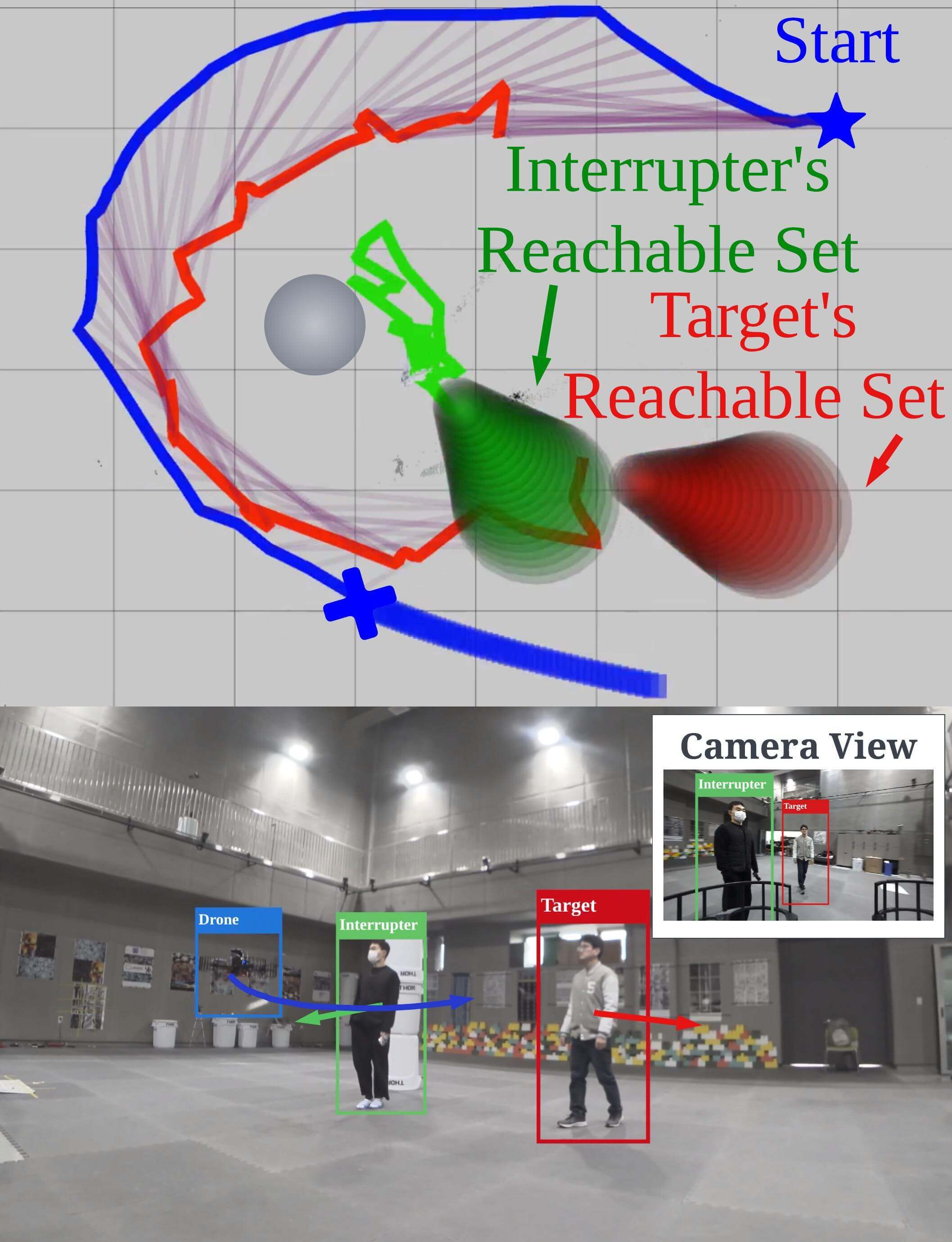
Refer to caption — (a) Single-target tracking

In order to address the factors above, we propose a real-time single- and dual-target tracking strategy that 1) can be adopted in both static and dynamic environments and 2) enhances the target visibility against prediction error, as illustrated in Fig. 1. The proposed method consists of two parts: prediction and chasing. In the prediction module, we calculate reachable sets of moving objects, taking into account the obstacle configuration. For efficient calculations, we use a sample-check strategy. First, we sample motion primitives representing possible trajectories, generated by quadratic programming (QP), which is solved in closed form. Then, collisions between primitives and obstacles are checked while leveraging the properties of Bernstein polynomials. We then calculate reachable sets enclosing the collision-free primitives.

In the chasing module, we design a chasing trajectory via a single QP. QP is known for being solvable in polynomial time and guaranteeing global optimality. We adopted this method because the optimization was solved within tens of milliseconds during numerous tests. The key idea of our trajectory planning is to define a target-visible region (TVR), a time-dependent spatial set that keeps the visibility of targets. Two essential factors of TVR enhance the target visibility. First, analyzing the topology of the targets’ path helps avoid situations where target occlusion inescapably occurs. Second, TVR is designed to maximize the visible area of the target’s reachable set, considering potential visual obstructions from obstacles and ensuring robust target visibility against the prediction error. Moreover, by allowing the entire target body to be viewed instead of specific points, the TVR enhances the target visibility. Additionally, to handle dual-target scenarios, we define an area where two targets can be simultaneously viewed with a limited FOV camera. Table I presents the comparison with the relevant works, and our main contributions are summarized as follows.

•

We propose a QP-based trajectory planning framework capable of single and dual target-chasing missions amidst static and dynamic obstacles, in contrast with existing works that address either single-target scenarios or static environments only.
•

(Prediction) We propose an efficient sample-check-based method to compute reachable sets of moving objects, leveraging Bernstein polynomials. This method reflects both static and dynamic obstacles, which contrasts with other works that do not fully consider the obstacle configurations in motion predictions.
•

(Chasing) We propose a target-visible trajectory generation method by designing a target-visible region (TVR), in which the target visibility is robustly maintained. This approach considers 1) the path topology, 2) the entire body of targets, and 3) the prediction error of moving objects. This contrasts with other works that fully trust potentially erroneous path predictions.

The remainder of this paper is arranged as follows. We review the relevant references in Section II, and the relationship between the target visibility and the path topology is studied in Section III. The problem statement and the pipeline of the proposed system are presented in Section IV, and Section V describes the prediction of the reachable set of moving objects. Section VI describes TVR, designs the reference trajectory for the chasing drone, and completes QP formulation. The validation of the proposed pipeline is demonstrated with high-fidelity simulations and real-world experiments in Section VII.

II Related Works

II-A Single Target Visibility against Static Obstacles

There have been various studies that take the target visibility into account in single-target chasing in static environments. [3] and [5] design cost functions that penalize target occlusion by obstacles, while [6] designs an environmental complexity cost function to adjust the distance between a target and a drone, implicitly reducing the probability of occlusion. These methods combine the functions with several other objective functions related to actuation efficiency and collision avoidance. Such conflicting objectives can yield a sub-optimal solution that compromises tracking motion. Therefore, the visibility of the target is not ensured. In contrast, our approach ensures the target visibility by incorporating it as a hard constraint in the QP problem, which can be solved quickly. On the other hand, there are works that explicitly consider visibility as hard constraints in optimization. [7] designs sector-shaped visible region and [8] designs select the view region among annulus sectors centered around the target. They use their target-visible regions in unconstrained optimization to generate a chasing trajectory. However, these works focus on the visibility of the center of a target, which may result in partial occlusion. In contrast, our method considers the visibility of the entire body of the target and accounts for the prediction error, thus enhancing robustness in target tracking.

Also, there are works that handle target path prediction for aerial tracking. [9] and [10] use past target observations to predict the future trajectory via polynomial regression. However, their method can generate erroneous results by insufficiently considering surroundings, resulting in path conflicts with obstacles. With inaccurate target path prediction, planners may not produce effective chasing paths and fail to chase a target without occlusion. Some works [11] and [12] predict the future target’s movements by formulating optimization problems that encourage the target to move towards free spaces. However, these approaches are limited to static environments. In contrast, our framework predicts the target’s movement considering both static and dynamic obstacles.

TABLE I: Comparison with the State-of-the-Art Algorithms.

Method	Scenarios		Prediction	Planning
Method	Dual-target	Dynamic obstacles	Environ. informed	PE-aware	WB of target
[11]	✕	✕	$\checkmark$	✕	✕
[13]	$\checkmark$	$\checkmark$	✕	✕	✓
[14]	✕	$\checkmark$	✕	✕	✕
[15]	✕	$\checkmark$	✕	✕	✕
[16]	✕	$\checkmark$	$\checkmark$	✕	✕
[17]	$\checkmark$	✕	$\checkmark$	✕	✕
[18]	$\checkmark$	✕	✕	✕	$\checkmark$
Ours	✔	✔	✔	✔	✔

$\checkmark$ means that the algorithm explicitly considers the corresponding item. (PE: Perception-error, and WB: Whole body)

II-B Single-Target Chasing in Dynamic Environments

Some studies treat tracking a target in dynamic environments. There are works that attempt to solve the occlusion problem by approximating the future motion of both dynamic obstacles and targets using a constant velocity model. [13] designs a target-visibility cost that is inspired by GPU ray casting model. [14] uses a learned occlusion model to evaluate the target visibility and tests the planner in dynamic environments. [15] aims to avoid occlusion by imposing a constraint that prevents a segment connecting a target and the drone from colliding with dynamic obstacles. Since [13] and [14] use the constant velocity model to predict the movements of dynamic objects, there are cases where the target and obstacles overlap, leading to incorrect target-visibility cost evaluation, which can ruin the planning results. Furthermore, the constraint in [15] cannot be satisfied if the predicted path of the target traverses occupied space (e.g. obstacles), which makes the optimization problem infeasible. In contrast, our approach predicts the movements of objects by fully considering the environment and incorporates the prediction error into planning to enhance the target visibility.

On the other hand, the approach in [16] makes a set of polynomial motion primitives and selects the best path under safety and target visibility constraints to acquire a non-colliding target path and generate a chasing trajectory. However, when the target and drone are near an obstacle, the planner [16] may select the path toward a region where occlusion is inevitable from the perspective of path topology, as will be shown in Section VII-C. In contrast, our method directly applies concepts of the path topology to prevent inescapable occlusion.

II-C Multiple Target Following

Multi-target tracking with a single drone has been discussed in a few works. [19] and [20] minimize the change in the target’s position in the camera image; however, they do not consider obstacles. [17] designs a dual visibility score field to handle the visibility of two targets among obstacles and a camera field-of-view (FOV) limit. Because the field is constructed heuristically, the success rate of tracking heavily depends on parameter settings. In contrast, our work handles these issues by applying them as hard constraints that must be satisfied. [18] tracks multiple targets by simultaneously controlling the camera’s intrinsic and extrinsic parameters. However, it is limited to systems where the intrinsic parameters can be controlled. In contrast, we consider the fixed and limited camera FOV with hard constraints to ensure the simultaneous observation of the targets.

II-D Target Following Using Quadratic Programming

Few aerial tracking works utilize QP for chasing trajectory planning: [12] and [21]. [12] calculates a series of viewpoints and uses QP optimization to interpolate them, but it does not ensure the target visibility when moving between the viewpoints. [21] generates safe flight corridors along the target’s path and pushes the drone’s trajectory toward the safe regions, but the target visibility is not considered in its QP problem. In contrast, we formulate the target visibility constraints for the full planning horizon. Also, in conventional drone trajectory generation methods using QP, the trajectory is confined to a specific part of the space over time intervals. However, by incorporating time-variant constraints, our method enables the drone to operate in a wider region, providing an advantage in target tracking.

III Preliminary

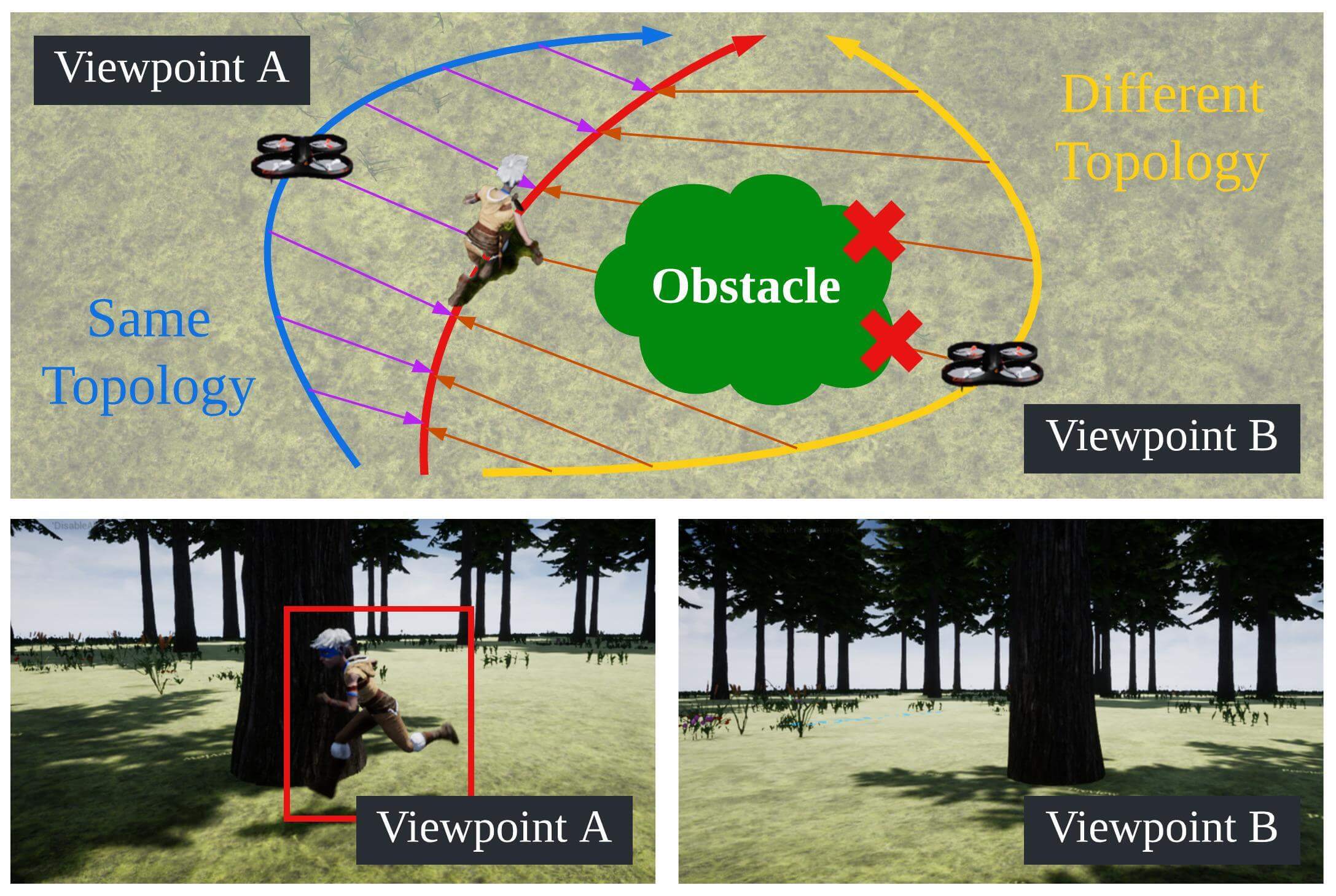
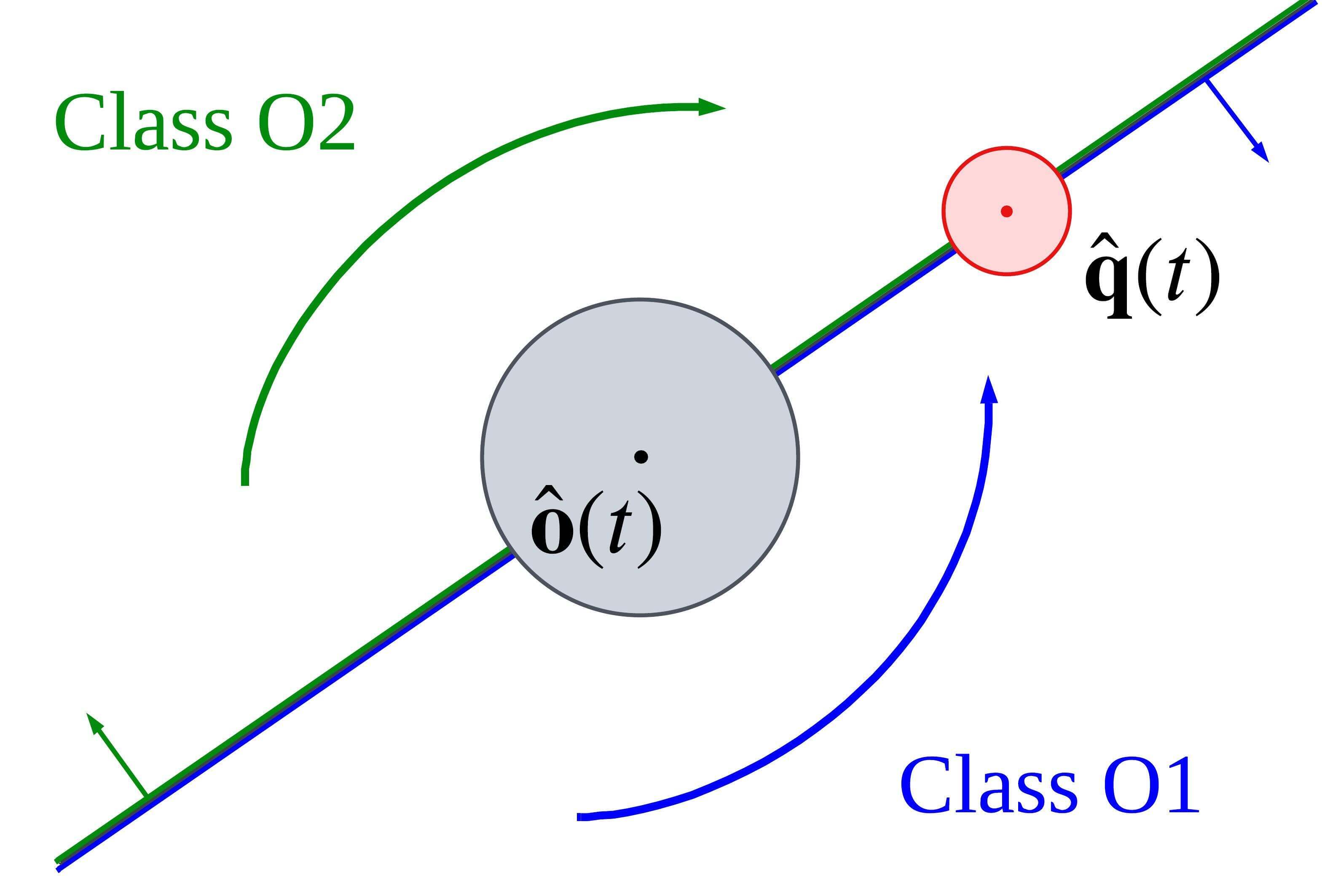
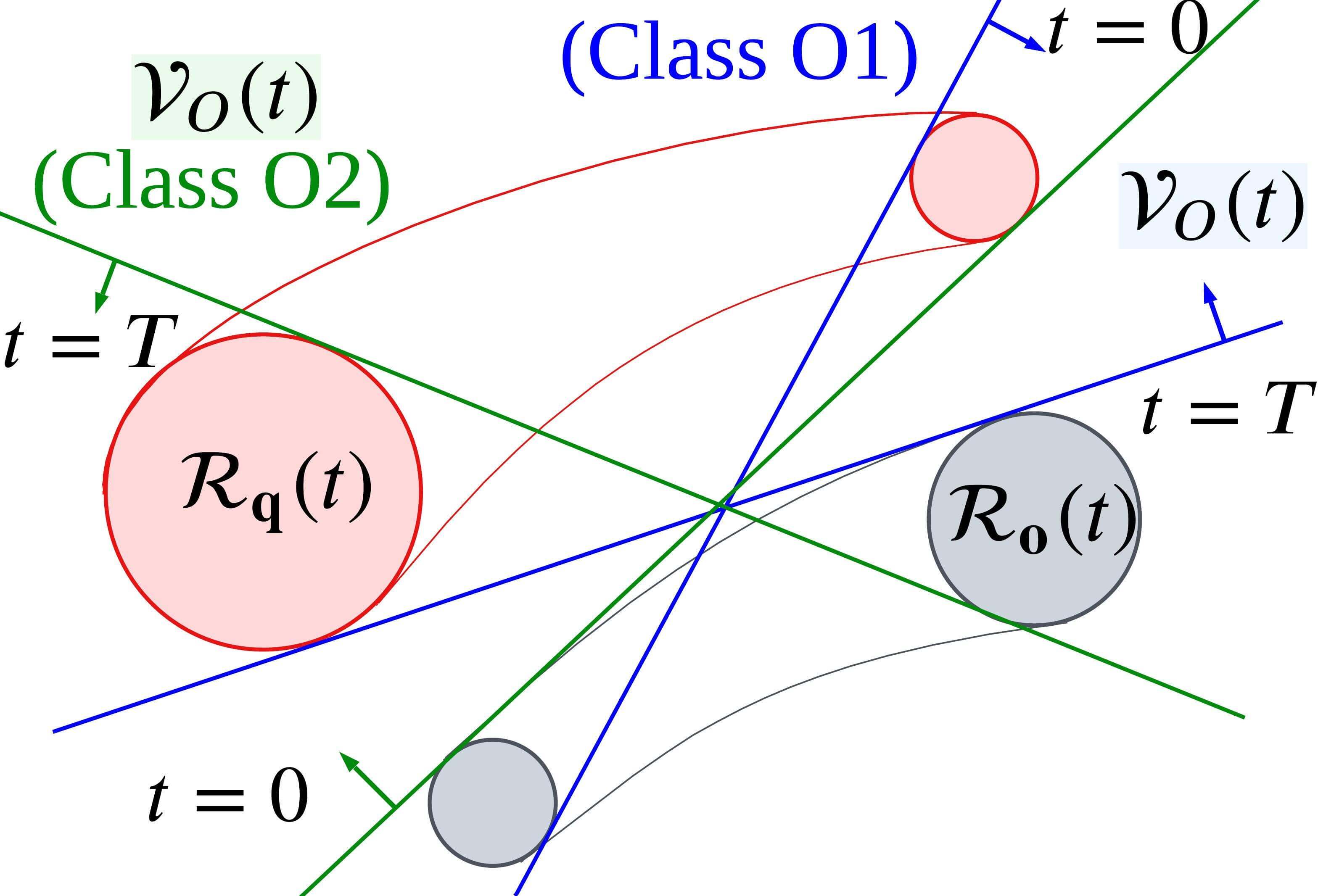
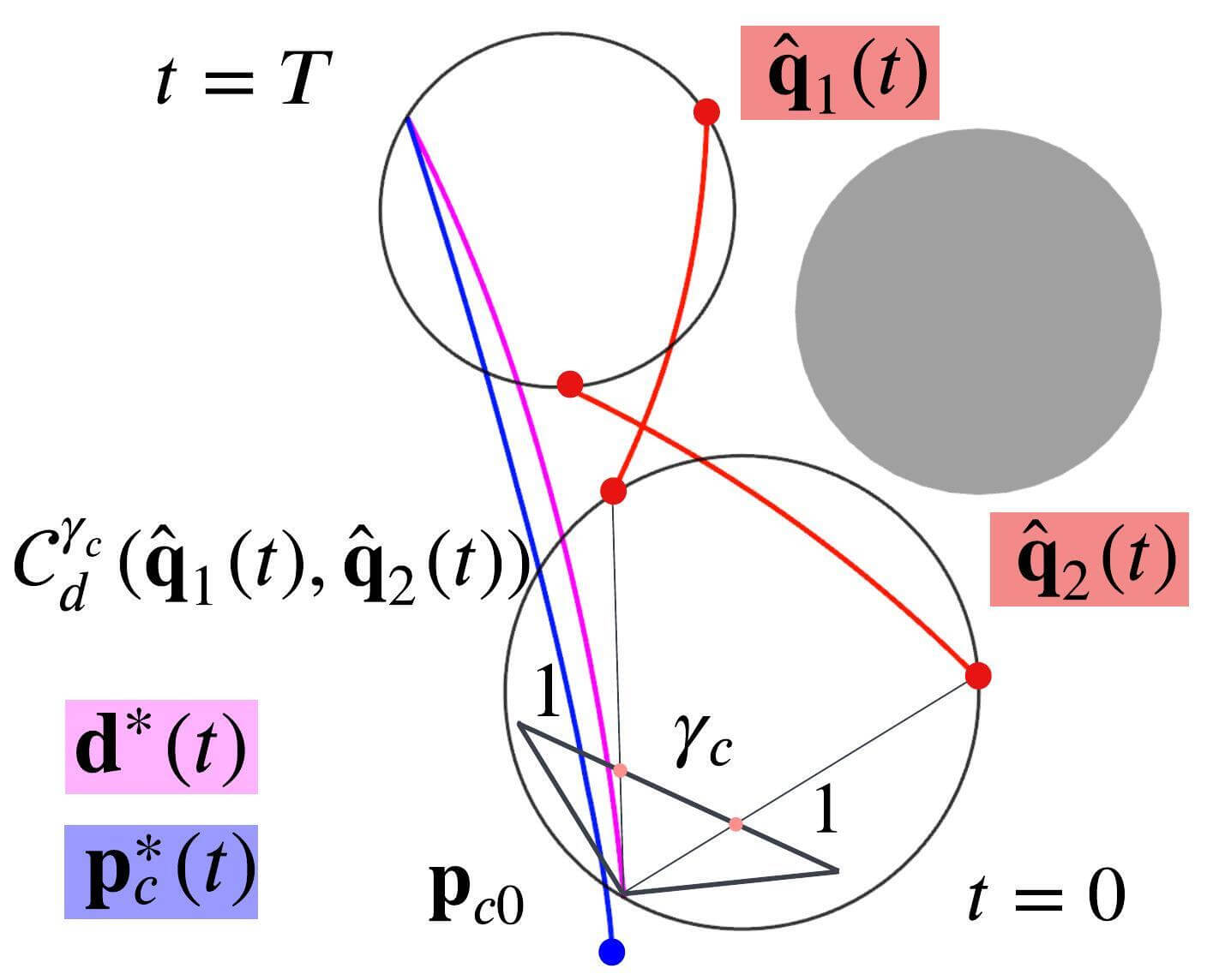
This section presents the relationship between target occlusion and path topology. In an obstacle environment, there exist multiple path topology classes [22]. As shown in Fig. 2, the visibility of the target is closely related to path topology. We analyze the relation between them and take it into consideration when generating the chasing trajectory.

As stated in [23], the definition of path homotopy is as follows.

Definition 1.

Paths $\sigma_{1},\sigma_{2}:I\to X\subset\mathbb{R}^{3}$ are path-homotopic if there is a continuous map $F:I\times I\to X$ such that

F(s,0)=\sigma_{1}(s)\ \text{and}\ F(s,1)=\sigma_{2}(s),

(1)

where $I$ is unit interval $[0,1]$ .

In this paper, Line-of-Sight is of interest, which is defined as follows.

Definition 2.

Line-of-Sight is a segment connecting two objects $\textbf{x}_{1},\textbf{x}_{2}:[0,\infty)\to\mathbb{R}^{3}$ .

\mathcal{L}(\textbf{x}_{1}(t),\textbf{x}_{2}(t))=(1-\epsilon)\textbf{x}_{1}(t)+\epsilon\textbf{x}_{2}(t),\quad\forall\epsilon\in I

(2)

where $t$ represents time.

Based on the definitions above, we derive a relation between the path topology and visibility between two objects.

Theorem 1.

When two objects are reciprocally visible, the paths of objects are path-homotopic.

Proof.

Suppose that two objects $\textbf{x}_{1}(t),\textbf{x}_{2}(t)$ move along paths $\sigma_{1},\sigma_{2}$ in free space $\mathcal{F}\subset\mathbb{R}^{3}$ during time interval $[t_{0},t_{f}]$ , respectively. i.e. $\sigma_{1}=\textbf{x}_{1}\circ\xi$ , $\sigma_{2}=\textbf{x}_{2}\circ\xi$ , where $\xi:I\to[t_{0},t_{f}]$ is the time mapping function such that $t=\xi(s)$ . If the visibility between $\textbf{x}_{1}$ and $\textbf{x}_{2}$ is maintained, the Line-of-Sight does not collide with obstacles: $\mathcal{L}(\textbf{x}_{1}(t),\textbf{x}_{2}(t))\subseteq\mathcal{F}$ for $\forall t\in[t_{0},t_{f}]$ . Then, by definition, $\mathcal{L}(\sigma_{1}(s),\sigma_{2}(s))=(1-\epsilon)\sigma_{1}(s)+\epsilon\sigma_{2}(s)\in\mathcal{F}$ for $\forall\epsilon,s\in I$ . Since such a condition satisfies the definition of continuous mapping in Definition 1, the two paths are homotopic. ∎

From Theorem 1, when the drone chooses a path with a different topology class from the target path, target occlusion inevitably occurs. Therefore, we explicitly consider path-homotopy when planning a chasing trajectory.

Throughout this article, we use the notation in Table II. The bold small letters represent vectors, calligraphic capital letters denote sets, and italic lowercase letters mean scalar values.

IV Overview

TABLE II: Nomenclature

Symbol	Definition
$\textbf{p}_{c}(t)$	A trajectory of the drone.
$\underline{\textbf{c}}$	An optimization variable that consists of Bernstein coefficients representing $\textbf{p}_{c}(t)$ .
$n_{c}$	The degree of a polynomial trajectory $\textbf{p}_{c}(t)$ .
$T$	Planning horizon
$\theta_{f}$	FOV of the camera built on the drone.
$v_{\text{max}},a_{\text{max}}$	The maximum speed and acceleration of the drone.
$\mathcal{F}$	Free space
$\boldsymbol{\mathcal{O}},\mathcal{O}_{j}$	A set of obstacles. An $j$ -th obstacle in $\mathcal{O}$
$N_{o},N_{samp}$	The number of elements of $\mathcal{O}$ and samples of end-points in the prediction.
$\mathcal{R}_{\textbf{q}_{j}}(t),\hat{\textbf{q}}_{j}(t),r_{q_{j}}(t)$	A reachable set of an $j$ -th target. A center trajectory and radius of $\mathcal{R}_{\textbf{q}_{j}}(t)$ . We omit a subscript $j$ to handle an arbitrary target.
$\mathcal{R}_{\textbf{o}_{j}}(t),\hat{\textbf{o}}_{j}(t),r_{o_{j}}(t)$	A reachable set of an $j$ -th obstacle. A center trajectory and radius of $\mathcal{R}_{\textbf{o}_{j}}(t)$ . We omit a subscript $j$ to handle an arbitrary obstacle.
$\mathcal{S}_{p},\mathcal{P}_{p},\mathcal{P}_{s}$	End Point Set, a set of candidate trajectories and a set of non-colliding candidate trajectories.
$\mathcal{L}(\textbf{x}_{1},\textbf{x}_{2})$	Line-of-Sight between $\textbf{x}_{1}$ and $\textbf{x}_{2}$ .
$\mathcal{V}_{O}(t),\mathcal{V}_{F}(t)$	Target visible region against a single obstacle (TVR-O) and target visible region that can see the two targets simultaneously with camera FOV (TVR-F).
$\mathcal{D}_{z}(t)$	A region where the drone cannot see both targets with the limited camera FOV.
$\psi(\textbf{p}_{c}(t);\hat{\textbf{q}}(t),\mathcal{O}_{i})$ , $\psi(\textbf{p}_{c}(t);\hat{\textbf{q}}(t),\mathcal{O})$	Visibility score against the $i$ -th obstacle. Visibility score against all obstacles.
${}_{\textbf{x}_{2}}\textbf{x}_{1}(t)$	Relative position between $\textbf{x}_{1}$ and $\textbf{x}_{2}$ at time $t$ . $\textbf{x}_{1}(t)-\textbf{x}_{2}(t)$ .
$\\|\textbf{x}\\|_{p}$	$L_{p}$ norm of x
$\textbf{x}^{\prime}(t),\textbf{x}^{\prime\prime}(t),\textbf{x}^{\prime\prime\prime}(t)$	First, second, third time derivatives of $\textbf{x}(t)$
$\textbf{a}^{\top},{B}^{\top}$	Transposed vector a and matrix $B$
$<,>,\leq,\geq$	elementwise inequality symbols
$\textbf{x}_{(x)},\textbf{x}_{(y)}$	$x$ - and $y$ -components of x.
$\begin{pmatrix}n\\ k\end{pmatrix}$	Binomial coefficients, the number of $k$ -combinations from a set of $n$ elements.
$\textbf{0}_{m\times n}$	An $m\times n$ matrix with all-zero elements.
$I_{m\times m}$	An identity matrix with rank $m$ .
$\text{det}(\cdot)$	Determinant of a matrix.
$\partial\mathcal{A}$	A boundary of a closed set $\mathcal{A}$ .
$\mathcal{B}(\textbf{x},r),\partial\mathcal{B}(\textbf{x},r)$	A ball with center at x and radius $r$ . A circumference of the ball.
$\|\mathcal{X}\|$	The number of elements in set $\mathcal{X}$
$\overline{AB}$ , $\angle{ABC}$	Segment connecting points $A$ and $B$ . Angle between $\overline{BA}$ and $\overline{BC}$ .

IV-A Problem Setup

In this section, we formulate the trajectory planning problem for a tracking drone with firmly attached camera sensors that have limited FOVs $\theta_{f}\in(0,\pi)$ [rad]. We consider an environment $\mathcal{W}$ , which consists of separate cylindrical static and dynamic obstacles. Our goal is to generate a trajectory of the drone so that it can see the single and dual targets ceaselessly in $\mathcal{W}$ over the time horizon $[0,T]$ . To achieve the goal, the drone has to predict the future movement of moving objects, such as targets and dynamic obstacles, and generate a target-chasing trajectory. To reflect the prediction error, we compute the reachable sets of moving objects. Then, based on the reachable sets, the planner generates a continuous-time trajectory that satisfies dynamical feasibility and avoids collision while preserving the target visibility. To accomplish the missions, we set up two problems: 1) Prediction problem and 2) Chasing problem.

IV-A1 Prediction problem

The prediction module forecasts reachable sets of moving objects such as targets and dynamic obstacles, over a time horizon $t\in[0,T]$ . The reachable sets $\mathcal{R}_{\textbf{q}}(t)$ and $\mathcal{R}_{\textbf{o}}(t)$ are sets that encompass the future positions of the targets $\textbf{q}(t)$ and obstacles $\textbf{o}(t)$ , respectively. The goal is to calculate the reachable sets considering an obstacle set $\mathcal{O}$ as well as estimation error. Specifically, we represent the $j$ -th target ( $j=1,2$ ) and $k$ -th obstacle ( $k\in\{1,\ldots,N_{o}:=|\mathcal{O}|\}$ ) as $\textbf{q}_{j}$ and $\textbf{o}_{k}$ respectively. Since the methods to compute $\mathcal{R}_{\textbf{o}}(t)$ and $\mathcal{R}_{\textbf{q}}(t)$ are equivalent, we use a symbol p instead of q and o to represent information of reachable sets of moving objects, in Section V.

IV-A2 Chasing problem

Given the reachable sets of the target and the obstacles obtained by the prediction module, we generate a trajectory of the drone $\textbf{p}_{c}(t)$ that keeps the target visibility from obstacles (3b), simultaneously sees the two targets with camera FOV $\theta_{f}$ in dual-target scenarios (3c), does not collide with obstacles (3d), and satisfies dynamical limits (3e)-(3f). For the smoothness of the trajectory and the high target visibility, the cost function (3a) consists of terms penalizing jerky motion ( $J_{j}$ ) and tracking error to designed reference trajectory ( $J_{e}$ ).


	$\displaystyle\underset{\textbf{p}_{c}(t)}{\text{min}}$	$\displaystyle J=w_{j}J_{j}+w_{e}J_{e}$	(3a)
	s.t.	$\displaystyle\mathcal{L}(\textbf{p}_{c}(t),\mathcal{R}_{\textbf{q}}(t))\subset\mathcal{F}\setminus\mathcal{R}_{\textbf{o}}(t)$	(3b)
$\displaystyle\cos^{-1}\bigg{(}\frac{{}_{\textbf{p}_{c}}\textbf{q}_{1}(t)^{\top}{}_{\textbf{p}_{c}}\textbf{q}_{2}(t)}{\\|{}_{\textbf{p}_{c}}\textbf{q}_{1}(t)\\|_{2}\\|{}_{\textbf{p}_{c}}\textbf{q}_{2}(t)\\|_{2}}\bigg{)}\leq\theta_{f}$			(3c)
$\displaystyle\mathcal{B}(\textbf{p}_{c}(t),r_{c})\subset\mathcal{F}\setminus\big{\{}\bigcup_{i=1}^{N_{o}}\mathcal{R}_{\textbf{o}_{i}}(t)\cup\mathcal{R}_{\textbf{q}}(t)\big{\}}$			(3d)
$\displaystyle\textbf{p}_{c}(0)=\textbf{p}_{c0},\ \textbf{p}_{c}^{\prime}(0)=\textbf{p}_{c0}^{\prime}$			(3e)
$\displaystyle\\|\textbf{p}_{c}^{\prime}(t)\\|_{2}\leq v_{\text{max}},\ \\|\textbf{p}_{c}^{\prime\prime}(t)\\|_{2}\leq a_{\text{max}}$			(3f)

where $w_{j}\geq 0$ and $w_{e}\geq 0$ are weight factors, ${}_{\textbf{p}_{c}}\textbf{q}_{j}(t)$ is the relative position between the drone and the $j$ -th target, $r_{c}$ is the radius of the drone, and $\textbf{p}_{c0}$ and $\textbf{p}_{c0}^{\prime}$ are current position and velocity of the drone, respectively. Section VI-D discusses the design of the chasing trajectory to maximize the target visibility, which is related to (3a). To handle (3b) and (3c), we design a target-visible region (TVR) in Section VI-B. (3d)-(3f) are addressed in Sections VI-C and VI-E.

IV-A3 Assumptions

For the Prediction problem, we assume that (AP1) the moving objects do not collide with obstacles, and (AP2) they do not move in a jerky way. In the Chasing problem, we assume that (AC1) the maximum velocity $v_{\text{max}}$ and the maximum acceleration $a_{\text{max}}$ of the drone are higher than the target and obstacles, and (AC2) the current state of drone does not violate (3b)-(3f). Furthermore, based on Theorem 1, when the targets move along paths with different path topology, occlusion unavoidably occurs, so we assume that (AC3) all targets move along homotopic paths against obstacles.
In addition, we set the flying height of the drone to a fixed level for the acquisition of consistent images of the target. From the problem settings, we focus on the design of chasing trajectory in the $x-y$ plane.

IV-A4 Trajectory representation

Due to the virtue of differential flatness of quadrotor dynamics [24], the trajectory of multi-rotors can be expressed with a polynomial function of time $t$ . In this paper, Bernstein basis is employed to express polynomials. Bernstein bases of $n$ -th order polynomial for time interval $[t_{a},t_{b}]$ are defined as follows:

b_{k,n}(t,t_{a},t_{b})=\begin{pmatrix}n\\ k\end{pmatrix}\frac{(t_{b}-t)^{n-k}(t-t_{a})^{k}}{(t_{b}-t_{a})^{n}},\ 0\leq k\leq n

(4)

Since the bases defined above are non-negative in the time interval $[t_{a},t_{b}]$ , a linear combination with non-negative coefficients makes the total value become non-negative. We utilize this property in the following sections.

The trajectory of the drone, $\textbf{p}_{c}(t)=[\textbf{p}_{c(x)}(t),\textbf{p}_{c(y)}(t)]^{\top}\in\mathbb{R}^{2}$ , is represented as an $M$ -segment piecewise Bernstein polynomial:

\textbf{p}_{c}(t)=\begin{cases}&\textbf{C}_{1}^{\top}\textbf{b}_{n_{c},1}(t)\ \ \ \ \ t\in[T_{0},T_{1}]\\ &\textbf{C}_{2}^{\top}\textbf{b}_{n_{c},2}(t)\ \ \ \ \ t\in[T_{1},T_{2}]\\ &\ldots\\ &\textbf{C}_{M}^{\top}\textbf{b}_{n_{c},M}(t)\ \ \ t\in[T_{M-1},T_{M}]\\ \end{cases}

(5)

where $T_{0}=0$ (current time), $T_{M}=T$ , $n_{c}$ is the degree of polynomial, $\textbf{C}_{m}=[\textbf{c}_{m(x)},\textbf{c}_{m(y)}]\in\mathbb{R}^{(n_{c}+1)\times 2}$ and $\textbf{b}_{n_{c},m}(t)=[b_{0,n_{c}}(t,T_{m-1},T_{m}),\ldots,b_{n_{c},n_{c}}(t,T_{m-1},T_{m})]^{\top}$ are control points and the corresponding basis vector of the $m$ -th segment, respectively. The array of control points in the $m$ -th segment is defined as $\textbf{c}_{m}=[\textbf{c}_{m(x)}^{\top},\textbf{c}_{m(y)}^{\top}]^{\top}\in\mathbb{R}^{2(n_{c}+1)}$ , and the concatenated vector of all control points $\underline{\textbf{c}}=[\textbf{c}_{1}^{\top},\ldots,\textbf{c}_{M}^{\top}]^{\top}\in\mathbb{R}^{2M(n_{c}+1)}$ is the decision variable of the polynomial trajectory optimization.

IV-A5 Objectives

For the Prediction Problem, the prediction module forecasts moving objects’ reachable set $\mathcal{R}_{\textbf{p}}(t)$ . Then, for the Chasing Problem, the chasing module formulates a QP problem with respect to $\underline{\textbf{c}}$ and finds an optimal $\underline{\textbf{c}}$ so that the drone chases the target without occlusion and collision while satisfying dynamical limits.

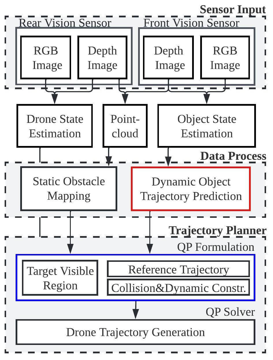
IV-B Pipeline

The overall architecture of QP Chaser is shown in Fig. 3. From cameras, RGB and depth images are acquired, and point cloud and information of target poses are extracted from the images. Then, locations and dimensions of static obstacles are estimated from the point cloud to build an obstacle map, and the reachable sets of the target and dynamic obstacles are predicted based on observed poses of the dynamic obstacles and the targets. Based on the static obstacle map and prediction results, the chasing trajectory for the drone is generated.

V Reachable Set Prediction

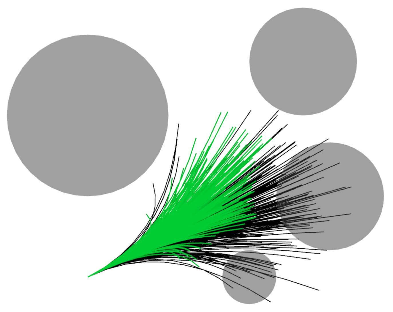
This section introduces a method for calculating reachable sets using the sample-check strategy. We sample a set of motion primitives and filter out the primitives that collide with obstacles. Then, we calculate a reachable set that encloses the remaining collision-free primitives. Figs. 4(a)-4(c) visualize the prediction process.

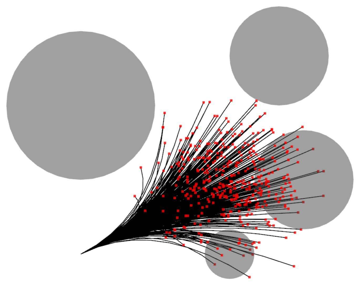
V-A Candidate for Future Trajectory of Moving Object

We sample the motion primitives of the target by collecting the positions that can be reached at $t=T$ and interpolating them with the current position.

V-A1 Endpoint sampling

The positions of a moving object at time $t=T$ are sampled, using a constant velocity model under disturbance:

		$\displaystyle\begin{bmatrix}\textbf{p}^{\prime}(t)\\ \textbf{p}^{\prime\prime}(t)\end{bmatrix}=F_{p}\begin{bmatrix}\textbf{p}(t)\\ \textbf{p}^{\prime}(t)\end{bmatrix}+G_{p}\textbf{w},\quad\textbf{w}\sim(0,Q),$		(6)
		$\displaystyle F_{p}=\begin{bmatrix}\textbf{0}_{2\times 2}&\textbf{I}_{2\times 2}\\ \textbf{0}_{2\times 2}&\textbf{0}_{2\times 2}\end{bmatrix},\quad G_{p}=\begin{bmatrix}\textbf{0}_{2\times 2}\\ \textbf{I}_{2\times 2}\end{bmatrix}$		(6)

where $\textbf{p}(t)\in\mathbb{R}^{2}$ is position of the moving object, and $\textbf{w}\in\mathbb{R}^{2}$ is white noise with power spectral density $Q$ . Then, with no measurement update, estimation error covariance $P(t)$ in continuous-time Kalman filter propagates with time [25].

P^{\prime}(t)=F_{p}(t)P(t)+P(t)F_{p}^{\top}(t)+G_{p}QG_{p}^{\top}

(7)

We collect $N_{samp}$ points from a 2-dimensional Gaussian distribution $\mathcal{N}\big{(}\int_{0}^{T}e^{-F_{p}(T-\tau)}[\hat{\textbf{p}}_{0}^{\top},\hat{\textbf{p}}_{0}^{\prime\top}]^{\top}d\tau,P(T)\big{)}$ , where $\hat{\textbf{p}}_{0}$ , $\hat{\textbf{p}}_{0}^{\prime}$ , and $P_{0}$ are position, velocity, and estimation error covariance at current time $t=0$ , respectively. We call the set of the samples the Endpoint Set:

\mathcal{S}_{p}=\{\textbf{s}_{p,i}\in\mathbb{R}^{2}|i=1,\ldots,N_{samp}\}.

(8)

V-A2 Primitive generation

Given the initial position, velocity, and end positions $\textbf{s}_{p,i}\in\mathcal{S}_{p}$ , we design trajectory candidates for moving objects. Under the assumption (AP2) that moving objects do not move in a jerky way, we establish the following problem.

		$\displaystyle\underset{\hat{\textbf{p}}_{i}(t)}{\text{min}}$		$\displaystyle\int_{0}^{T}\\|\hat{\textbf{p}}_{i}^{\prime\prime\prime}(t)\\|^{2}_{2}dt$		(9)
		s.t.		$\displaystyle\hat{\textbf{p}}_{i}(0)=\hat{\textbf{p}}_{0},\ \hat{\textbf{p}}_{i}^{\prime}(0)=\hat{\textbf{p}}_{0}^{\prime},\ \hat{\textbf{p}}_{i}(T)=\textbf{s}_{p,i}$		(9)

Recalling that the trajectory is represented with Bernstein polynomial, we write an $i$ -th candidate trajectory as $\hat{\textbf{p}}_{i}(t)=\textbf{P}^{\top}_{i}\textbf{b}_{n_{p}}(t)$ , $i=1,\ldots,N_{samp}$ where $\textbf{P}_{i}=[\textbf{p}_{i(x)},\textbf{p}_{i(y)}]\in\mathbb{R}^{(n_{p}+1)\times 2}$ and $\textbf{b}_{n_{p}}(t)=[b_{0,n_{p}}(t,0,T),\ldots,b_{n_{p},n_{p}}(t,0,T)]^{\top}$ . By defining $\underline{\textbf{p}}_{i}:=[\textbf{p}_{i(x)}^{\top},\textbf{p}_{i(y)}^{\top}]^{\top}$ as an optimization variable, (9) becomes a QP problem

		$\displaystyle\underset{\underline{\textbf{p}}_{i}}{\text{min}}$		$\displaystyle\frac{1}{2}\underline{\textbf{p}}_{i}^{\top}Q_{p}\underline{\textbf{p}}_{i}$		(10)
		s.t.		$\displaystyle A_{p}\underline{\textbf{p}}_{i}=\textbf{b}_{p,i}$		(10)

where $Q_{p}$ is a positive semi-definite matrix, $A_{p}$ is a $6\times(n_{p}+1)$ matrix, and $\textbf{b}_{p,i}$ is a vector composed of $\hat{\textbf{p}}_{0}$ , $\hat{\textbf{p}}_{0}^{\prime}$ , and $\textbf{s}_{p,i}$ . (10) can be converted into unconstrained QP, whose optimal $\textbf{p}_{i}$ is a closed-form solution as follows.

\begin{bmatrix}\underline{\textbf{p}}_{i}\\ \boldsymbol{\lambda}\end{bmatrix}=\begin{bmatrix}Q_{p}&A_{p}^{\top}\\ A_{p}&\textbf{0}_{6\times 6}\end{bmatrix}^{-1}\begin{bmatrix}\textbf{0}_{2(n_{p}+1)\times 1}\\ \textbf{b}_{p,i}\end{bmatrix}

(11)

where $\boldsymbol{\lambda}$ is a lagrange multiplier. A set of candidate trajectories of the moving object is defined as $\mathcal{P}_{p}$ .

V-B Collision Check

Under the assumption (AP1) that moving objects do not collide, trajectory candidates $\hat{\textbf{p}}_{i}(t)\in\mathcal{P}_{p}$ that violate the below condition are filtered out.

\|\hat{\textbf{p}}_{i}(t)-\textbf{o}_{j}(t)\|_{2}^{2}-(r_{p0}+r_{o_{j}}(t))^{2}\geq 0,\ \forall t\in[0,T]

(12)

Due to the fact that all terms in (12) can be represented in polynomials, and Bernstein bases are non-negative in the time period $[0,T]$ , entirely non-negative coefficients make the left-hand side of (12) non-negative. We examine all coefficients of (12) for the primitives belonging to $\mathcal{P}_{p}$ . For details, see Appendix A. We call a set of primitives that pass the test $\mathcal{P}_{s}$ .

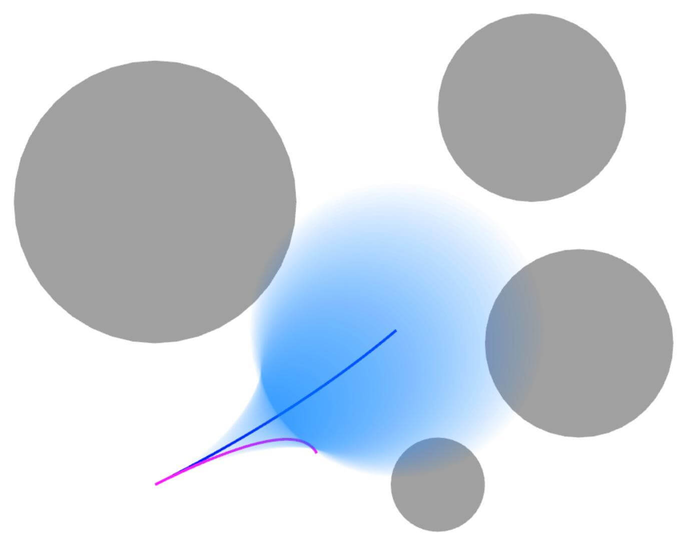
V-C Prediction with Error Bounds

With the set $\mathcal{P}_{s}$ , the reachable set $\mathcal{R}_{\textbf{p}}(t)$ is defined as a time-varying ball enclosing all the primitives in $\mathcal{P}_{s}$ .

\mathcal{R}_{\textbf{p}}(t)=\mathcal{B}(\hat{\textbf{p}}(t),r_{p}(t))

(13)

We determine a center trajectory $\hat{\textbf{p}}(t)$ as the primitive with the smallest sum of distances to the other primitives in $\mathcal{P}_{s}$ :

\hat{\textbf{p}}(t)=\underset{\hat{\textbf{p}}_{i}(t)\in\mathcal{P}_{s}}{\text{argmin}}\sum_{j\neq i}^{|\mathcal{P}_{p}|}\int_{0}^{T}\|\hat{\textbf{p}}_{i}(t)-\hat{\textbf{p}}_{j}(t)\|_{2}dt.

(14)

Proposition 1.

The optimization problem (14) is equivalent to the following problem.

		$\displaystyle\hat{\textbf{p}}(t)=\hat{\textbf{p}}_{i^{}}(t),\ i^{}=\underset{i}{\text{argmin}}\sum_{j=0}^{\|\mathcal{P}_{p}\|}\\|\textbf{s}_{p,i}-\textbf{s}_{p,j}\\|_{2},$		(15)
		$\displaystyle\text{where}\ \hat{\textbf{p}}_{i}(t),\hat{\textbf{p}}_{j}(t)\in\mathcal{P}_{s}$		(15)

Proof.

See Appendix B. ∎

From Proposition 1, $\hat{\textbf{p}}(t)$ is determined by simple arithmetic operations and the process has a time complexity of $O(|\mathcal{P}_{s}|^{2})$ . Then, we define $r_{p}(t)$ so that $\mathcal{R}_{\textbf{p}}(t)$ encloses all the primitives in $\mathcal{P}_{s}$ for $\forall{t}\in[0,T]$ .

r_{p}(t)=\underset{\hat{\textbf{p}}_{j}(t)\in\mathcal{P}_{s}}{\max}\|\hat{\textbf{p}}(t)-\hat{\textbf{p}}_{j}(t)\|_{2}+r_{p0}

(16)

The second term in the right hand side of (16) allows the whole body to be contained in $\mathcal{R}_{\textbf{p}}(t)$ . The use of $r_{q}(t)$ and $r_{o}(t)$ in chasing problem allows for the consideration of the visibility of the entire bodies of the targets, as well as the potential movements of moving targets and dynamic obstacles.

V-D Evaluation

We measure the computation time of prediction in obstacle environments. We set $n_{p}$ as 3 and test 1000 times for different scenarios $(N_{samp},N_{o})=$ (500,2), (500,4), (2000,2), (2000,4). The prediction module is computed on a laptop with an Intel i7 CPU, with a single thread implementation, and execution time is summarized in Table III. As $N_{samp}$ and $N_{o}$ increase, the time needed for calculating primitives and collision checks increases. However, obstacles that are close to $\mathcal{P}_{p}$ make $|\mathcal{P}_{s}|$ small. Accordingly, the time to compute a reachable set decreases as the number of close obstacles increases.

TABLE III: Computation Time in Prediction Process

(N_{samp},N_{o})

(500,2)

(500,4)

(2000,2)

(2000,4)

Endpoints Sampling &

Primitive Generation [

\mu

43.97

47.23

168.3

184.1

Collision Check [

\mu

146.3

185.3

487.9

750.7

Reachable Set

Computation [ms]

0.245

0.172

2.921

2.073

Total Time [ms]

0.435

0.405

3.577

3.008

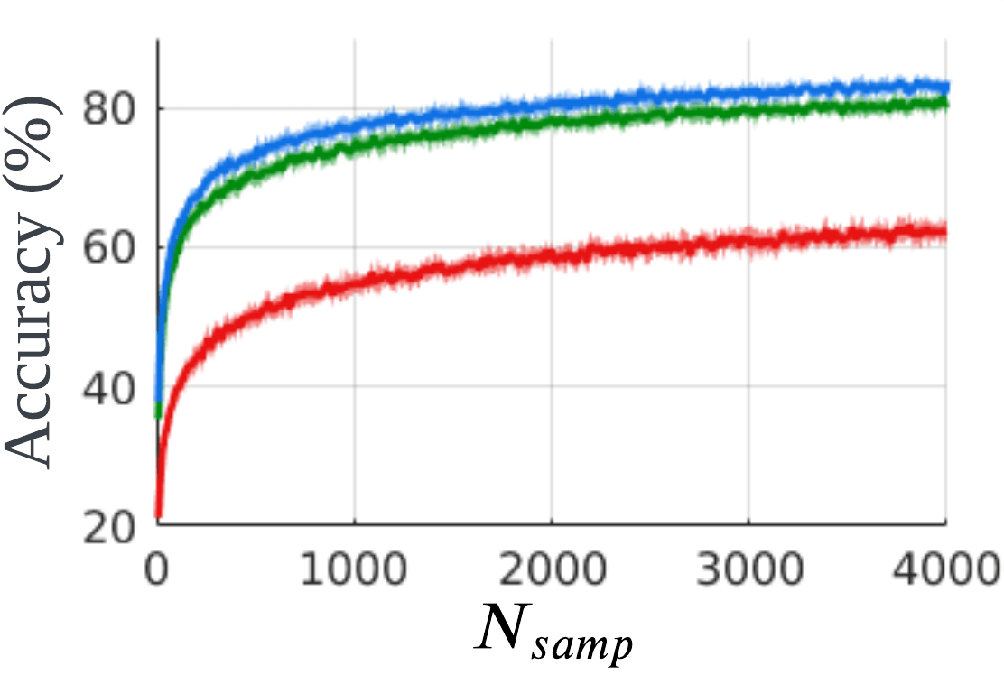
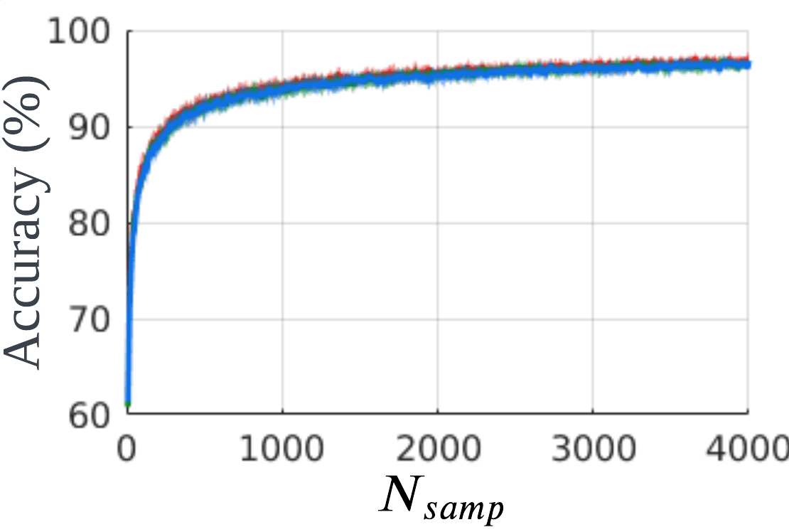
Also, we test the accuracy of the presented prediction methods. For evaluation, discretized models of (6) with power spectral density of white noise $Q=$ 0.1, 0.5, 1.0 $[\text{m}^{2}/\text{s}^{3}]$ are considered. We confirm whether $\mathcal{B}(\textbf{p}(t),r_{p0})\subset\mathcal{R}_{\textbf{p}}(t)$ is satisfied in obstacle-free situations while progressively increasing the $N_{samp}$ . For each $N_{samp}$ , the tests are executed 10000 times, and the acquired accuracy is shown in Fig. 5. Contrary to the assumption (AP2) that a moving object moves smoothly, the discretized model can move in a jerky way. Therefore, since the proposed method cannot describe jerky movements during certain initial time intervals, we excluded some initial parts from the tests. As $N_{samp}$ increases, the accuracy improves, but the computation time increases, as presented in Table III. Therefore, $N_{samp}$ should be determined according to the computation resources for a balance between accuracy and running time. In this paper, we set $N_{samp}$ as 2000. With this setting, $\mathcal{B}(\textbf{p}(t),r_{p0})\subset\mathcal{R}_{\textbf{p}}(t)$ , $\forall t\in(0,T]$ was satisfied 98.8% empirically in the simulations in Section VII-C.

As elaborated in Section IV-A, we specifically calculate the reachable sets of moving targets and obstacles: $\mathcal{R}_{\textbf{q}}(t)=\mathcal{B}(\hat{\textbf{q}}(t),r_{q}(t))$ and $\mathcal{R}_{\textbf{o}}(t)=\mathcal{B}(\hat{\textbf{o}}(t),r_{o}(t))$ . Subsequently, in the following section, we generate a trajectory that maximizes the visibility of $\mathcal{R}_{\textbf{q}}(t)$ while avoiding $\mathcal{R}_{\textbf{o}}(t)$ .

VI Chasing Trajectory Generation

This section formulates a QP problem to make a chasing trajectory occlusion-free, collision-free, and dynamically feasible. We first define the target visible region (TVR), the region with maximum visibility of the target’s reachable set, and formulate constraints regarding collision avoidance and dynamic limits. Then, we design the reference trajectory to enhance the target visibility. Regarding the target visibility, all the steps are based on the path topology.

VI-A Topology Check

In 2-dimensional space, there exist two classes of path topology against a single obstacle, as shown in Fig. 6(a). As stated in Theorem 1, the drone should move along a homotopic path with the target path to avoid occlusion. Based on the relative position between the drone and the obstacle, ${}_{\hat{\textbf{o}}}\textbf{p}_{c}(t)=\textbf{p}_{c}(t)-\hat{\textbf{o}}(t)$ , and the relative position between the target and the obstacle, ${}_{\hat{\textbf{o}}}\hat{\textbf{q}}(t)=\hat{\textbf{q}}(t)-\hat{\textbf{o}}(t)$ , at the current time $t=0$ , the topology class of chasing path is determined as follows.

\begin{cases}&\textit{Class O1}\ (\text{if}\ \det\begin{bmatrix}{}_{\hat{\textbf{o}}}\textbf{p}_{c}^{\top}(0)\\ {}_{\hat{\textbf{o}}}\hat{\textbf{q}}^{\top}(0)\end{bmatrix}\geq 0)\\ &\textit{Class O2}\ (\text{if}\ \det\begin{bmatrix}{}_{\hat{\textbf{o}}}\textbf{p}_{c}^{\top}(0)\\ {}_{\hat{\textbf{o}}}\hat{\textbf{q}}^{\top}(0)\end{bmatrix}<0)\\ \end{cases}

(17)

After conducting the topology check above, we define the visibility constraint and reference chasing trajectory.

VI-B Target Visible Region

To robustly maintain the target visibility despite the prediction error, the target visible region TVR is defined considering the reachable sets of the moving objects: $\mathcal{R}_{\textbf{q}}(t)$ and $\mathcal{R}_{\textbf{o}}(t)$ .

VI-B1 Target visibility against obstacles

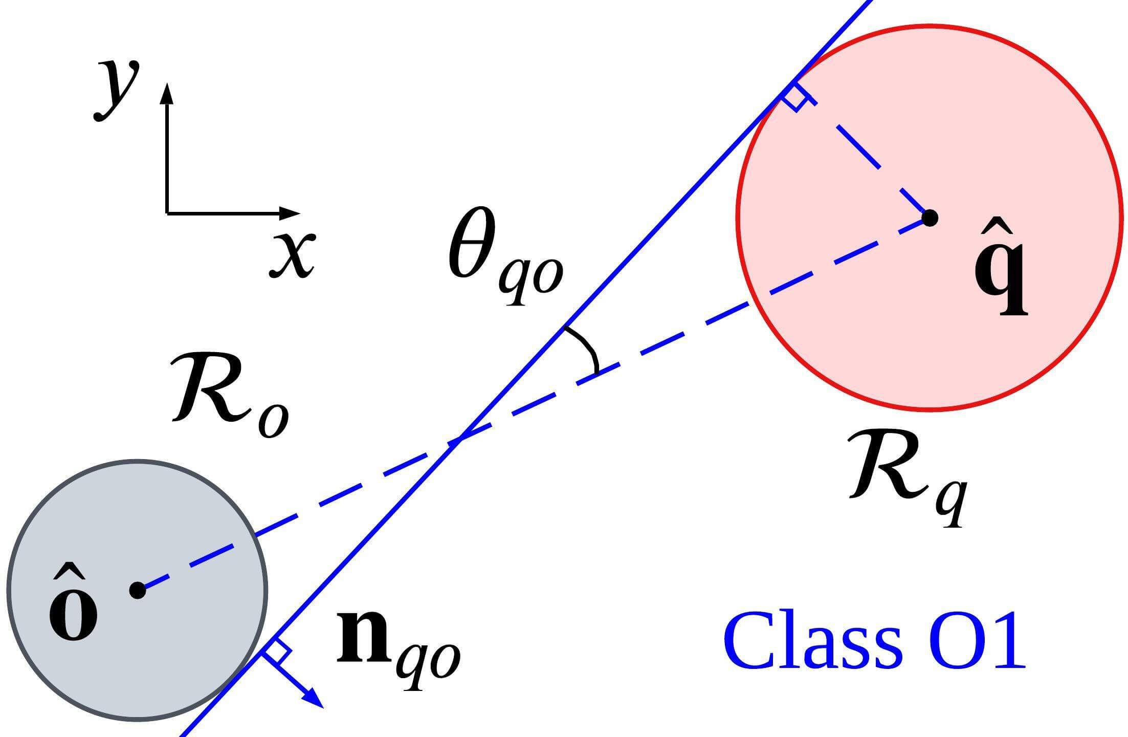
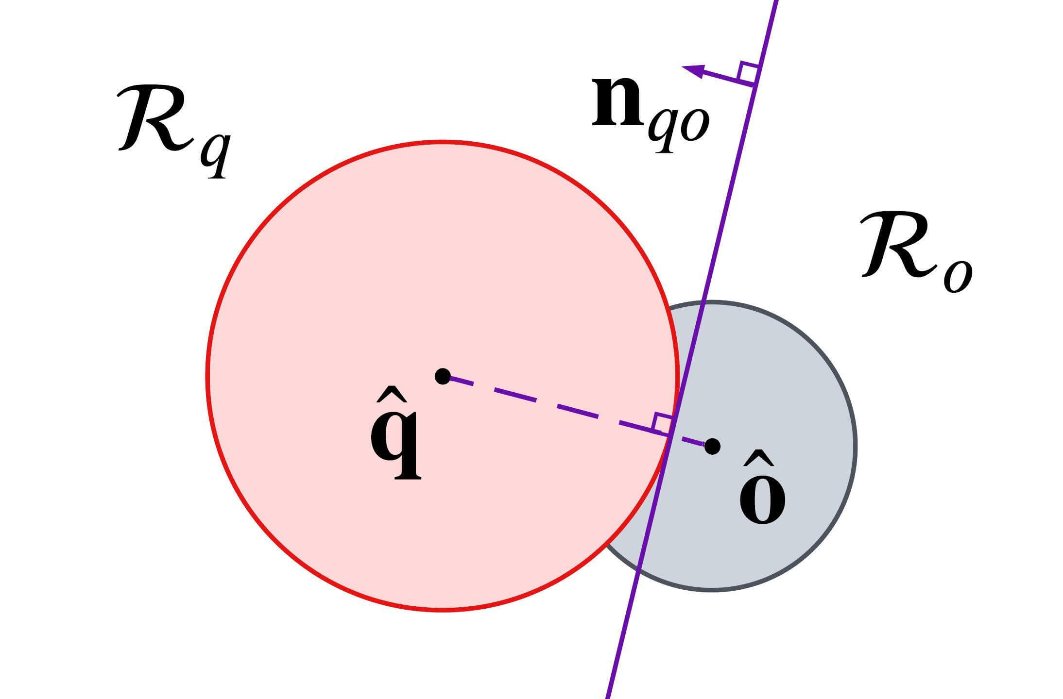
We define the target visible region against an obstacle (TVR-O), for each obstacle. To maximize a visible area of the targets’ reachable set that is not occluded by the reachable set of obstacles, TVR-O is set to a half-space so that it includes the target’s reachable set and minimizes the area that overlaps with the obstacle’s reachable set. There are two cases where the reachable sets of the target and obstacles overlap and do not overlap, and TVR-O is defined accordingly.

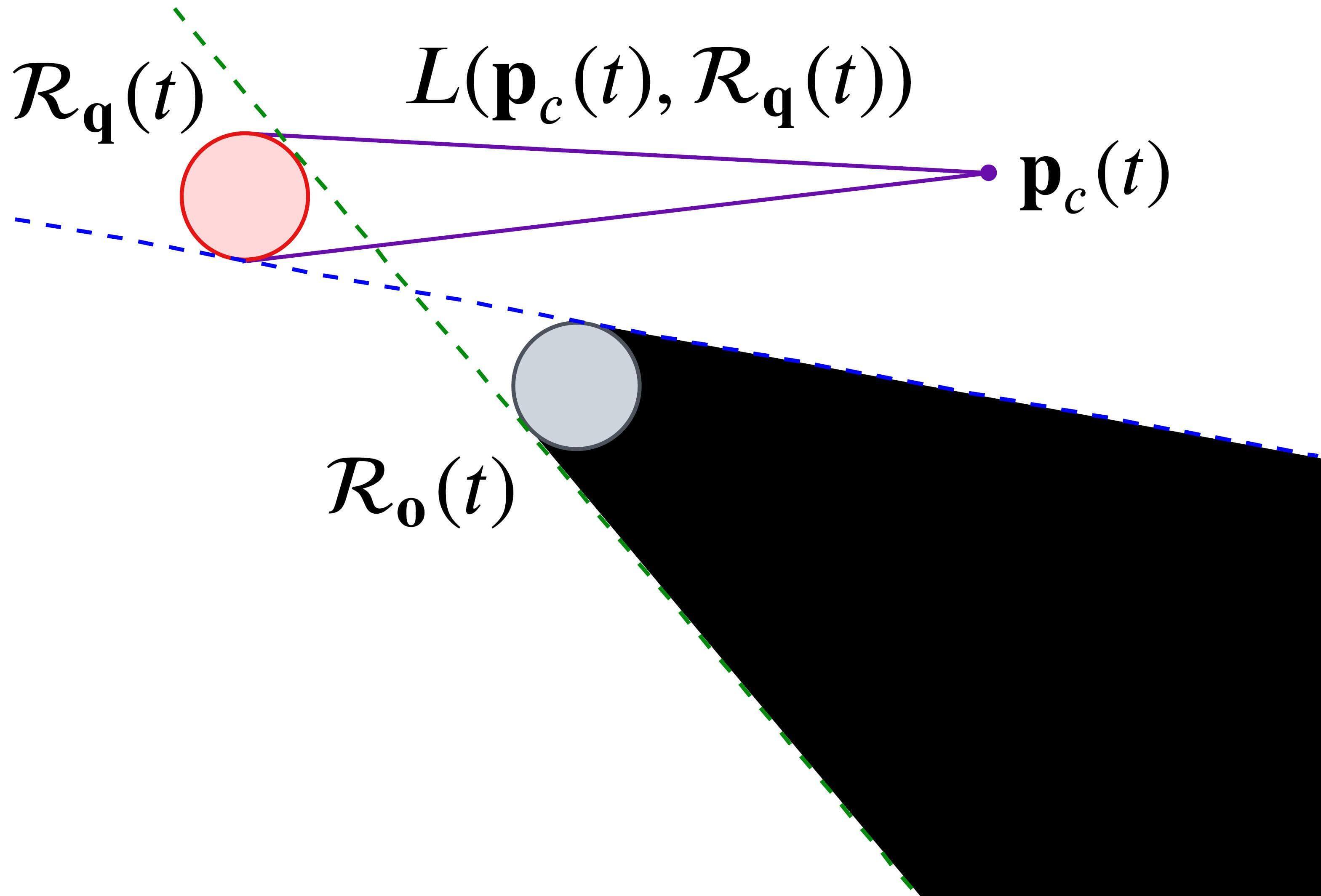
Case 1: In the case where the reachable sets of the target and an obstacle do not overlap, the target invisible region is made by straight lines which are tangential to both $\mathcal{R}_{\textbf{q}}(t)$ and $\mathcal{R}_{\textbf{o}}(t)$ , as shown in Fig. 6(b). Accordingly, we define TVR-O as a half-space made by a tangential line between $\mathcal{R}_{\textbf{q}}(t)$ and $\mathcal{R}_{\textbf{o}}(t)$ according to the topology class (17), as shown in Fig. 6(c). $\mathcal{V}_{O}(t)$ denotes TVR-O and is represented as follows.

	$\displaystyle\mathcal{V}_{O}(t)=\Big{\{}\textbf{x}(t)\in\mathbb{R}^{2}\|\ {}_{\hat{\textbf{o}}}\hat{\textbf{q}}^{\top}(t)\begin{bmatrix}r_{qo}(t)&\mp d_{2}(t)\\ \pm d_{2}(t)&r_{qo}(t)\end{bmatrix}{}_{\hat{\textbf{o}}}\textbf{x}(t)$		(18)
	$\displaystyle-r_{o}(t)d_{1}^{2}(t)\geq 0\Big{\}}$		(18)

where $r_{qo}(t)=r_{q}(t)+r_{o}(t)$ , $d_{1}(t)=\|{}_{\hat{\textbf{o}}}\hat{\textbf{q}}(t)\|_{2}$ , and $d_{2}(t)=(d_{1}^{2}(t)-r_{qo}^{2}(t))^{\frac{1}{2}}$ . The double signs in (18) are in the same order, where the lower and upper signs are for Class O1 and Class O2, respectively.

Lemma 1.

If $\textbf{p}_{c}(t)\in\mathcal{V}_{O}(t)$ , $\mathcal{L}(\textbf{p}_{c}(t),\mathcal{R}_{\textbf{q}}(t))\subset\mathcal{F}\setminus\mathcal{R}_{\textbf{o}}(t)$ is satisfied.

Proof.

$\mathcal{V}_{O}(t)$ is a half-space which is convex, and both $\textbf{p}_{c}(t)$ and $\mathcal{R}_{\textbf{q}}(t)$ belong to $\mathcal{V}_{O}(t)$ . By the definition of convexity, all the Lines-of-Sight connecting the drone $\textbf{p}_{c}(t)$ and all points in the reachable set of the target $\mathcal{R}_{\textbf{q}}(t)$ are included in $\mathcal{V}_{O}(t)$ . Since the TVR-O defined in (18) is disjoint with $\mathcal{R}_{\textbf{o}}(t)$ , $\mathcal{L}(\textbf{p}_{c}(t),\mathcal{R}_{\textbf{q}}(t))\subset\mathcal{F}\setminus\mathcal{R}_{\textbf{o}}(t)$ . ∎

Remark 1.

In dual-target scenarios, in order to avoid the occlusion of a target by another target, (18) is additionally defined by considering one of the targets as an obstacle.

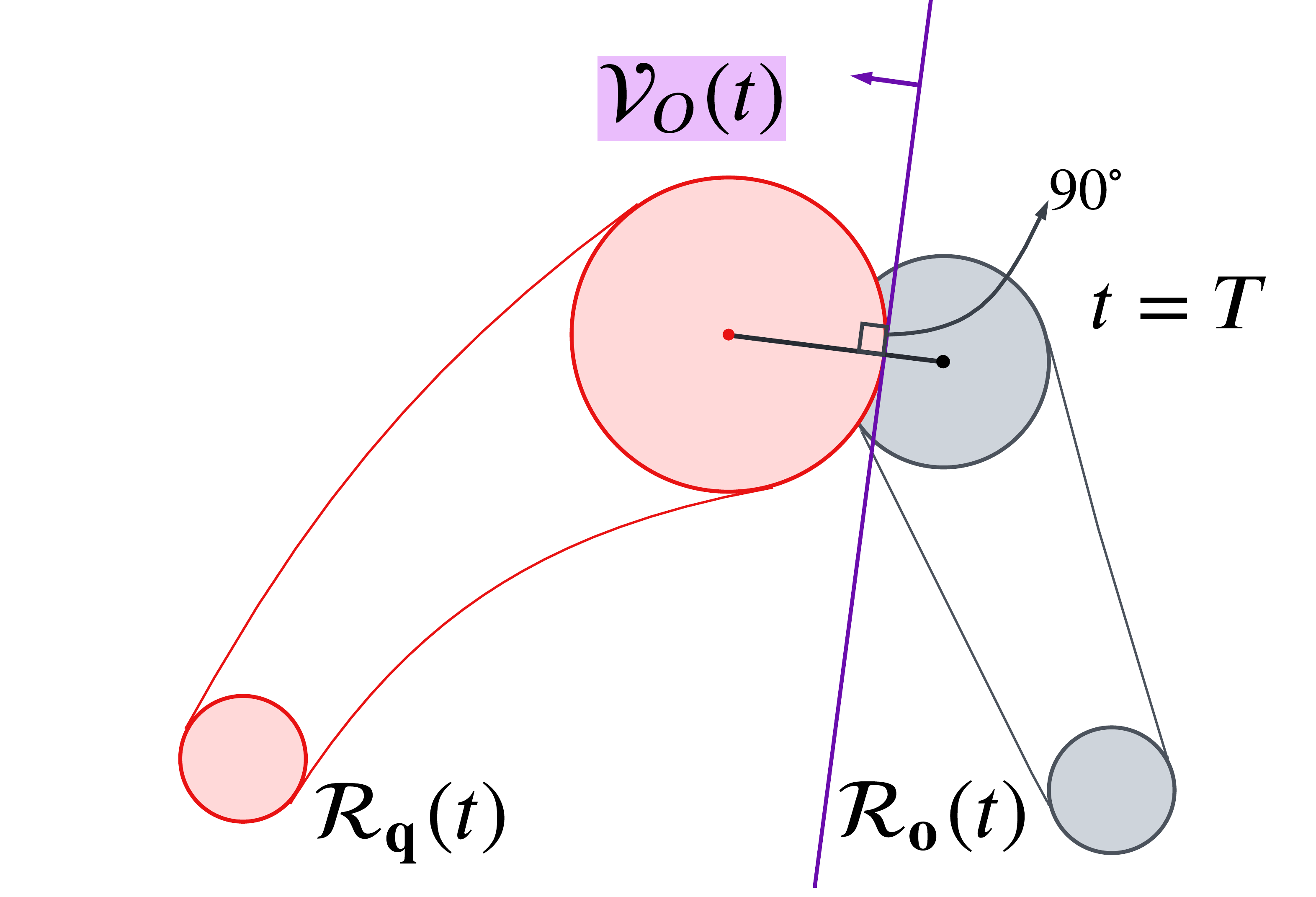
Case 2: For the case where the reachable sets overlap, TVR-O becomes a half-space made by a tangential line to $\mathcal{R}_{\textbf{o}}(t)$ , which is perpendicular to a line segment connecting the centers of the target $\hat{\textbf{q}}(t)$ and the obstacles $\hat{\textbf{o}}(t)$ , illustrated as straight lines in Fig. 6(d). Then the TVR-O is represented as

\mathcal{V}_{O}(t)=\{\textbf{x}(t)\in\mathbb{R}^{2}|{}_{\hat{\textbf{o}}}\hat{\textbf{q}}^{\top}(t){}_{\hat{\textbf{q}}}\textbf{x}(t)+r_{q}(t)d_{1}(t)\geq 0\}

(19)

The reachable sets include the volumes of the moving objects along with the prediction error. Since TVR-O is defined based on the reachable sets, it enhances the visibility of the entire body of the target against the prediction error. For detailed formulations of (18) and (19), see Appendix C-A.

VI-B2 Bernstein polynomial approximation

In defining TVR-O, all terms in (18)-(19) are polynomials except $d_{1}(t)$ and $d_{2}(t)$ . To make $\textbf{p}_{c}(t)\in\mathcal{V}_{O}(t)$ affine with respect to the optimization variable $\underline{\textbf{c}}$ , we first convert $d_{1}(t),d_{2}(t)$ into Bernstein polynomials using the following numerical technique that originates from Lagrange interpolation with standard polynomial representation [26].
For the time interval $[T_{m-1},T_{m}]$ , $d_{l}(t)$ , $l=1,2$ are approximately represented as $\tilde{d}_{l,m}(t)=\sum_{j=0}^{\tilde{n}_{l}}\tilde{d}_{l,m,j}b_{j,\tilde{n}_{l}}(t,T_{m-1},T_{m})$ . $\tilde{n}_{l}$ is the degree of $\tilde{d}_{l,m}(t)$ , and control points $\tilde{\textbf{d}}_{l,m}=[\tilde{d}_{l,m,0},\ldots,\tilde{d}_{l,m,\tilde{n}_{l}}]^{\top}$ can be acquired as follows:

\tilde{\textbf{d}}_{l,m}=B_{\tilde{n}_{l}}^{-1}\bar{\textbf{d}}_{l,m}

(20)

where $B_{\tilde{n}_{l}}=\{b_{j,k}\}\in\mathbb{R}^{(\tilde{n}_{l}+1)\times(\tilde{n}_{l}+1)}$ is a Bernstein-Vandermonde matrix [27] with elements given by $b_{j,k}=\begin{pmatrix}\tilde{n}_{l}\\ k\end{pmatrix}$ ${\Big{(}\dfrac{j}{\tilde{n}_{l}}\Big{)}}^{k}{\Big{(}\dfrac{\tilde{n}_{l}-j}{\tilde{n}_{l}}\Big{)}}^{\tilde{n}_{i}-k},\ 0\leq j,k\leq\tilde{n}_{l}$ , and $\bar{\textbf{d}}_{l,m}\in\mathbb{R}^{\tilde{n}_{l}+1}$ consists of $\tilde{n}_{l}+1$ sequential samples $d_{l}\big{(}(1-\frac{n}{\tilde{n}_{l}})T_{m-1}+\frac{n}{\tilde{n}_{l}}T_{m}\big{)},\ 0\leq n\leq\tilde{n}_{l}$ .
With the approximated terms $\tilde{d}_{1}(t),\tilde{d}_{2}(t)$ , we represent the target visibility constraint as follows.


		$\displaystyle\textbf{Case 1}:\ t\in[T_{m-1},T_{m}],\ \text{s.t. }\mathcal{R}_{\textbf{q}}(t)\cap\mathcal{R}_{\textbf{o}}(t)=\emptyset:$		(21a)
		$\displaystyle\quad\quad{}_{\hat{\textbf{o}}}\hat{\textbf{q}}^{\top}(t)\begin{bmatrix}r_{qo}(t)&\mp\tilde{d}_{2}(t)\\ \pm\tilde{d}_{2}(t)&r_{qo}(t)\end{bmatrix}{}_{\hat{\textbf{o}}}\textbf{p}_{c}(t)-r_{o}(t){d}_{1}^{2}(t)\geq 0$
		$\displaystyle\textbf{Case 2}:\ t\in[T_{m-1},T_{m}],\ \text{s.t. }\mathcal{R}_{\textbf{q}}(t)\cap\mathcal{R}_{\textbf{o}}(t)\neq\emptyset:$		(21b)
		$\displaystyle\quad\quad{}_{\hat{\textbf{o}}}\hat{\textbf{q}}^{\top}(t){}_{\hat{\textbf{q}}}\textbf{p}_{c}(t)-r_{q}(t)\tilde{d}_{1}(t)\geq 0$

VI-B3 FOV constraints

In addition to (21), the drone should avoid the region where it cannot see the two targets with its limited camera FOV. As shown in Fig. 6(e), circles whose inscribed angle of an arc tracing points $Q_{1}$ and $Q_{2}$ at $\hat{\textbf{q}}_{1}(t)$ , $\hat{\textbf{q}}_{2}(t)$ equals $\theta_{f}$ , are represented as follows.

		$\displaystyle\mathcal{D}_{j}(t)=\mathcal{B}(\textbf{f}_{j}(t),r_{f}(t)),\ j=1,2\ ,$		(22)
		$\displaystyle\textbf{f}_{j}(t)=\frac{1}{2}\begin{bmatrix}1&(-1)^{j+1}\cot{\theta_{f}}\\ (-1)^{j}\cot{\theta_{f}}&1\end{bmatrix}{}_{\hat{\textbf{q}}_{1}}\hat{\textbf{q}}_{2}(t)+\hat{\textbf{q}}_{1}(t),$
		$\displaystyle r_{f}(t)=\frac{1}{2\sin{\theta_{f}}}\\|{}_{\hat{\textbf{q}}_{1}}\hat{\textbf{q}}_{2}(t)\\|_{2},\ {}_{\hat{\textbf{q}}_{1}}\hat{\textbf{q}}_{2}(t)=\hat{\textbf{q}}_{2}(t)-\hat{\textbf{q}}_{1}(t)$

According to the geometric property of an inscribed angle, $\angle Q_{1}XQ_{2}>\theta_{f}$ , $\angle Q_{1}YQ_{2}<\theta_{f}$ for $\forall X\in\mathcal{D}_{z}(t)\setminus\partial\mathcal{D}_{z}(t)$ , $\forall Y\notin\mathcal{D}_{z}(t)$ , where $D_{z}(t)$ is represented as follows.

\mathcal{D}_{z}(t)=\begin{cases}&\mathcal{D}_{1}(t)\cap\mathcal{D}_{2}(t)\quad(\text{if}\ \theta_{f}\geq\frac{\pi}{2})\\ &\mathcal{D}_{1}(t)\cup\mathcal{D}_{2}(t)\quad(\text{if}\ \theta_{f}<\frac{\pi}{2})\end{cases}

(23)

Since the camera FOV is $\theta_{f}$ , the drone inside $\mathcal{D}_{z}(t)$ misses at least one target in the camera image inevitably, and the drone outside of $\mathcal{D}_{z}(t)$ is able to see both targets.

We define the target visible region considering camera FOV (TVR-F) as a half-space that does not include $\mathcal{D}_{z}(t)$ and is tangential to $\mathcal{D}_{z}(t)$ , as shown in Fig. 6(e). $\mathcal{V}_{F}(t)$ denotes TVR-F and is represented as follows.

\mathcal{V}_{F}(t)=\{\textbf{x}(t)|\pm\text{det}(\begin{bmatrix}{}_{\hat{\textbf{q}}_{1}}\textbf{x}^{\top}(t)\\ {}_{\hat{\textbf{q}}_{1}}\hat{\textbf{q}}_{2}^{\top}(t)\end{bmatrix})-\frac{1+\cos{\theta_{f}}}{2\sin{\theta_{f}}}\|{}_{\hat{\textbf{q}}_{1}}\hat{\textbf{q}}_{2}(t)\|_{2}^{2}\geq 0\}

(24)

The upper and lower signs in (24) are for Class F1 and Class F2, respectively, which are defined as

\begin{cases}&\textit{Class F1}\ (\text{if}\ \det\begin{bmatrix}{}_{\hat{\textbf{q}}_{1}}\textbf{p}_{c}^{\top}(0)\\ {}_{\hat{\textbf{q}}_{1}}\hat{\textbf{q}}_{2}^{\top}(0)\end{bmatrix}\geq 0)\\ &\textit{Class F2}\ (\text{if}\ \det\begin{bmatrix}{}_{\hat{\textbf{q}}_{1}}\textbf{p}_{c}^{\top}(0)\\ {}_{\hat{\textbf{q}}_{1}}\hat{\textbf{q}}_{2}^{\top}(0)\end{bmatrix}<0).\end{cases}

(25)

We enforce the drone to satisfy $\textbf{p}_{c}(t)\in\mathcal{V}_{F}(t)$ in order to see both targets. For the details, see the Appendix C-B.

VI-C Collision Avoidance

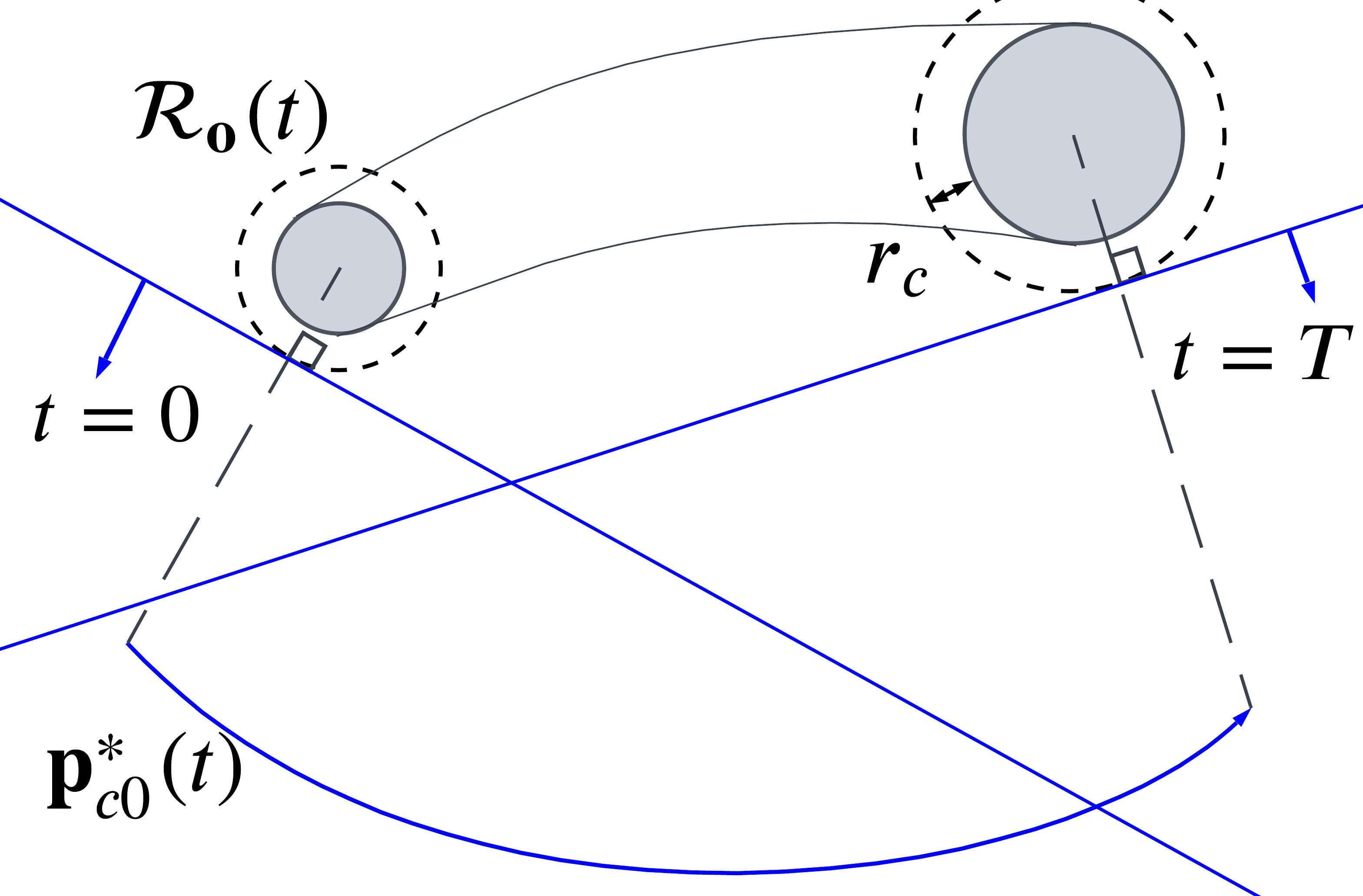
To avoid collision with obstacles, we define a collision-free area as a half-space made by a tangential line to a set that is inflated by $r_{c}$ from $\mathcal{R}_{\textbf{o}}(t)$ . The tangential line is drawn considering a trajectory $\textbf{p}_{c0}^{*}(t)$ , which is the previous planning result. This is illustrated in Fig. 6(f) and represented as follows.

\mathcal{F}_{c}(t)=\{\textbf{x}(t)\in\mathbb{R}^{2}|{}_{\hat{\textbf{o}}}\textbf{p}_{c0}^{*T}(t){}_{\hat{\textbf{o}}}\textbf{x}(t)\geq(r_{o}(t)+r_{c})\|{}_{\hat{\textbf{o}}}\textbf{p}_{c0}^{*}(t)\|_{2}\}

(26)

where ${}_{\hat{\textbf{o}}}\textbf{p}_{c0}^{*}(t):=\textbf{p}_{c0}^{*}(t)-\hat{\textbf{o}}(t)$ . As in (20), we approximate a non-polynomial term $\|{}_{\hat{\textbf{o}}}\textbf{p}_{c0}^{*}(t)\|_{2}$ to a polynomial $\tilde{d}_{3}(t)$ . With the approximated term $\tilde{d}_{3}(t)$ , the collision constraint is defined as follows:

{}_{\hat{\textbf{o}}}\textbf{p}_{c0}^{*T}(t){}_{\hat{\textbf{o}}}\textbf{p}_{c}(t)-(r_{o}(t)+r_{c})\tilde{d}_{3}(t)\geq 0

(27)

Due to the fact that the multiplication of Bernstein polynomials is also a Bernstein polynomial, the left-hand side of the (21), (24), and (27) can be represented in a Bernstein polynomial form. With the non-negativeness of Bernstein basis, we make coefficients of each basis non-negative in order to keep the left-hand side non-negative, and (21), (24), and (27) turn into affine constraints with the decision vector $\underline{\textbf{c}}$ . The constraints can be written as follows, and we omit details.

$\displaystyle A_{\text{TVR-O}}\underline{\textbf{c}}-\textbf{b}_{\text{TVR-O}}$	$\displaystyle\geq 0,$	(28)
$\displaystyle A_{\text{TVR-F}}\underline{\textbf{c}}-\textbf{b}_{\text{TVR-F}}$	$\displaystyle\geq 0,$
$\displaystyle A_{\text{Colli}}\underline{\textbf{c}}-\textbf{b}_{\text{Colli}}$	$\displaystyle\geq 0$

VI-D Reference Trajectory for Target Tracking

In this section, we propose a reference trajectory for target chasing that enhances the visibility of the targets.

VI-D1 Single-target case

In designing the reference trajectory, we use the visibility score, which is computed based on the Euclidean Signed Distance Field (ESDF), as discussed in [28]. The definition of the visibility score is the closest distance between all points in an $j$ -th obstacle, $\mathcal{O}_{j}$ , and the Line-of-Sight connecting the target and the drone:

\psi(\textbf{p}_{c}(t);\hat{\textbf{q}}(t),\mathcal{O}_{j})=\min_{\textbf{x}\in\mathcal{L}(\textbf{p}_{c}(t),\hat{\textbf{q}}(t))}\phi(\textbf{x},\mathcal{O}_{j}).

(29)

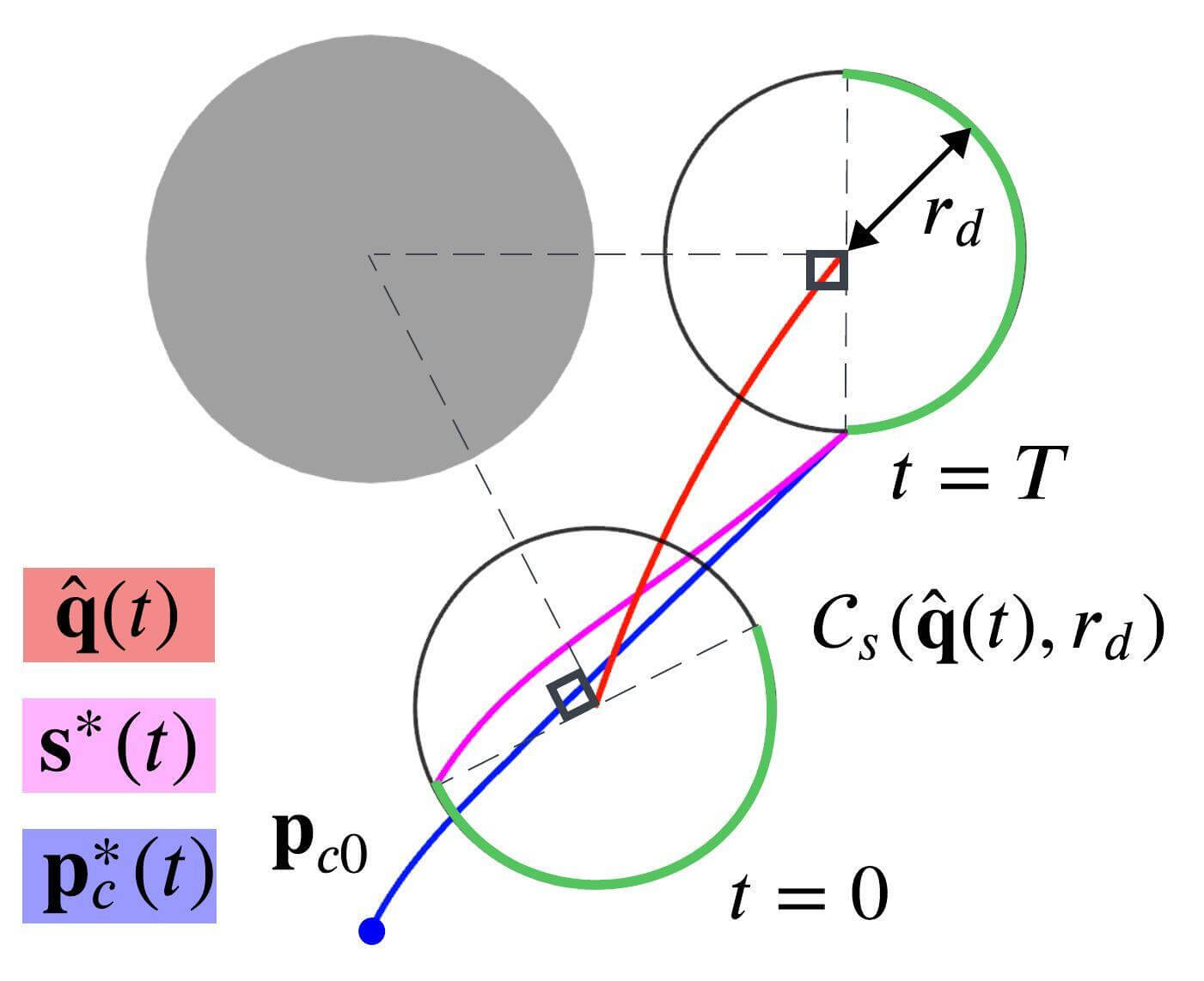
In order to keep the projected size of the target on the camera image, we set the desired shooting distance $r_{d}$ . With the desired shooting distance $r_{d}$ , a viewpoint candidate set can be defined as $\mathcal{C}_{s}(\hat{\textbf{q}}(t),r_{d})$ $=\partial\mathcal{B}(\hat{\textbf{q}}(t),r_{d})$ . Under the assumption that the environment consists of cylindrical obstacles, half-circumference of $\mathcal{C}_{s}(\hat{\textbf{q}}(t),r_{d})$ acquires the maximum visibility score, as illustrated in green in Fig. 7(a). Therefore, the following trajectory maintains the maximum $\psi(\textbf{p}_{c}(t);\hat{\textbf{q}}(t),\mathcal{O}_{j})$ .

\textbf{s}_{j}(t)=\textbf{q}(t)+r_{d}[\cos{\delta_{j}(t)},\sin{\delta_{j}(t)}]^{\top}

(30)

where $\delta_{j}(t)=\tan^{-1}({}_{\hat{\textbf{o}}_{j}}\hat{\textbf{q}}_{(y)}(t))/{}_{\hat{\textbf{o}}_{j}}\hat{\textbf{q}}_{(x)}(t))\mp\frac{\pi}{2}$ . The upper and lower signs are for Class O1 and Class O2, respectively. We define the reference trajectory as a weighted sum of $\textbf{s}_{j}(t)$ .

\textbf{s}^{*}(t)=\Big{(}\sum_{j=1}^{N_{o}}w_{s,j}\Big{)}^{-1}\sum_{j=1}^{N_{o}}w_{s,j}\textbf{s}_{j}(t)

(31)

$w_{s,j}$ ’s are weight functions that are inversely proportional to the current distance between the target and each obstacle.

VI-D2 Dual-target case

In order to make aesthetically pleasing scenes, we aim to place two targets in a ratio of $1:\gamma_{c}:1$ on the camera image. To do so, the drone must be within a set $\mathcal{C}_{d}^{\gamma_{c}}(\hat{\textbf{q}}_{1}(t),\hat{\textbf{q}}_{2}(t))$ , which is defined as follows and illustrated as a black circle in Fig. 7(b).

		$\displaystyle\mathcal{C}_{d}^{\gamma_{c}}(\hat{\textbf{q}}_{1}(t),\hat{\textbf{q}}_{2}(t))=\partial\mathcal{B}(\textbf{f}_{c}(t),r_{f,c}(t)),$		(32)
		$\displaystyle\textbf{f}_{c}(t)=\frac{1}{2}(\hat{\textbf{q}}_{1}(t)+\hat{\textbf{q}}_{2}(t))\pm$
		$\displaystyle\quad\frac{\gamma_{c}+2}{4\gamma_{c}}\cot{\frac{\theta_{f}}{2}}\Big{(}1-\frac{\gamma_{c}^{2}}{(\gamma_{c}+2)^{2}}\tan^{2}{\frac{\theta_{f}}{2}}\Big{)}\begin{bmatrix}0&1\\ -1&0\end{bmatrix}{}_{\hat{\textbf{q}}_{1}}\hat{\textbf{q}}_{2}(t),$
		$\displaystyle r_{f,c}(t)=\frac{\gamma_{c}+2}{4\gamma_{c}}\cot{\frac{\theta_{f}}{2}}\Big{(}1+\frac{\gamma_{c}^{2}}{(\gamma_{c}+2)^{2}}\tan^{2}{\frac{\theta_{f}}{2}}\Big{)}\\|{}_{\hat{\textbf{q}}_{1}}\hat{\textbf{q}}_{2}(t)\\|_{2}$

The upper and lower signs are for Class F1 and Class F2. We define the reference trajectory to acquire a high visibility score $\psi$ while maintaining the ratio.

		$\displaystyle\textbf{d}^{*}(t)=\textbf{f}_{c}(t)+r_{f,c}(t)[\cos{\delta_{d}}(t),\sin{\delta_{d}(t)}]^{\top},$		(33)
		$\displaystyle\delta_{d}(t)=\tan^{-1}{\frac{\sum_{j=1}^{2N_{o}}w_{s,j}\sin{\delta_{j}(t)}+w_{b}\sin{\delta_{b}(t)}}{\sum_{j=1}^{2N_{o}}w_{s,j}\cos{\delta_{j}(t)}+w_{b}\cos{\delta_{b}(t)}}}$		(33)

$\delta_{b}(t)=\tan^{-1}({}_{\hat{\textbf{q}}_{1}}\hat{\textbf{q}}_{2(y)}(t))/{}_{\hat{\textbf{q}}_{1}}\hat{\textbf{q}}_{2(x)}(t))\mp\frac{\pi}{2}$ , and $w_{s,j}$ and $\delta_{j}(t)$ are defined as in (30), for two targets. The upper and lower signs are for Class F1 and Class F2, respectively. $\delta_{b}(t)$ is defined as the farthest direction from the two targets to maximize a metric, $\psi(\textbf{p}_{c}(t);\hat{\textbf{q}}_{1}(t),\hat{\textbf{q}}_{2}(t))$ + $\psi(\textbf{p}_{c}(t);\hat{\textbf{q}}_{2}(t),\hat{\textbf{q}}_{1}(t))$ , representing the visibility score between two targets.

For the numerical stability of the QP solver, the reference trajectory is redefined by interpolating between $\boldsymbol{\mu}^{*}(t)$ , $\boldsymbol{\mu}=\textbf{s},\textbf{d}$ and the current drone’s position $\textbf{p}_{c0}$ . With a non-decreasing polynomial function $\alpha(t)$ that satisfies $\alpha(0)=0$ and $\alpha(T)=1$ , the reference trajectory is defined as follows.

\textbf{p}_{c}^{*}(t)=\big{(}1-\alpha(t)\big{)}\textbf{p}_{c0}+\alpha(t)\boldsymbol{\mu}^{*}(t)

(34)

Since trigonometric terms for $\boldsymbol{\mu}^{*}(t)$ , $\boldsymbol{\mu}=$ s or d in (31), (33) are non-polynomial, the Lagrange interpolation is used as (20). The approximated $\textbf{p}_{c}^{*}(t)$ is denoted as $\tilde{\textbf{p}}_{c}^{*}(t)$ . Based on the construction of reference trajectory and the target visibility constraints, we formulate the trajectory optimization problem as a QP problem.

VI-E QP Formulation

VI-E1 Trajectory segmentation

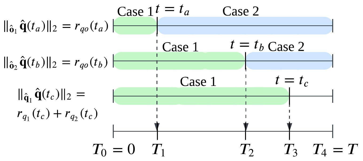
The constraint (21) is divided into the cases: when the reachable sets are separated and when they overlap. To apply (21) according to the situation, the roots of two equations $\|{}_{\hat{\textbf{o}}}\hat{\textbf{q}}(t)\|_{2}=r_{qo}(t)$ and $\|{}_{\hat{\textbf{q}}_{1}}\hat{\textbf{q}}_{2}(t)\|_{2}=r_{q1}(t)+r_{q2}(t)$ should be investigated for $t\in(0,T)$ . We define $[T_{0},\ldots,T_{M}]$ by arranging the roots of the above equations in ascending order, and we set $M$ time intervals, as stated in (5). Fig. 8 visualizes the above process. Thanks to De Casteljau’s algorithm [29], the single Bernstein polynomial such as $\hat{\textbf{q}}(t),\hat{\textbf{o}}(t),r_{q}(t),r_{o}(t)$ can be divided into $M$ Bernstein polynomials. Using an $M$ -segment-polynomial representation, we formulate a QP problem.

VI-E2 Constraints

The drone’s trajectory should be dynamically feasible, (3e) and (3f), while maintaining the target visibility, (3b) and (3c), and avoiding collision, (3d). To construct the QP problem, we formulate the constraints to be affine with respect to $\underline{\textbf{c}}$ . By leveraging the properties of Bernstein polynomials, which include P1) the first and last coefficients corresponding to the endpoints and P2) the convex hull property, we can effectively formulate dynamic constraints. Also, the $l$ -th derivative of an $n$ -th order Bernstein polynomial is an $(n-l)$ -th order polynomial. The coefficients of the $l$ -th derivative of a polynomial are obtained by multiplying the coefficients of the original polynomial by the following matrix.

	$\displaystyle E_{n,m}^{(l)}$	$\displaystyle=\begin{cases}\frac{n-l+1}{T_{m}-T_{m-1}}E_{n-l}E_{n,m}^{(l-1)}&\text{if}\ l\geq 1\\ \textbf{I}_{(n+1)\times(n+1)}&\text{if}\ l=0\end{cases},\ n\geq l\geq 0,$		(35)
	$\displaystyle E_{l}$	$\displaystyle=\begin{bmatrix}-1&1&0&\dotsi&0\\ 0&\ddots&\ddots&\ddots&\vdots\\ \vdots&\ddots&\ddots&\ddots&0\\ 0&\dotsi&0&-1&1\end{bmatrix}\in\mathbb{R}^{l\times(l+1)}$		(35)

First, the trajectory is made to satisfy the initial condition, (3e): current position and velocity. Using P1), we can get


	$\displaystyle\textbf{e}_{n_{c}+1,1}^{\top}E_{n_{c},m}^{(0)}\textbf{C}_{m}=\textbf{p}_{c0}^{\top},$		(36a)
	$\displaystyle\textbf{e}_{n_{c},1}^{\top}E_{n_{c},m}^{(1)}\textbf{C}_{m}=\textbf{p}_{c0}^{\prime\top},$		(36b)

where $\textbf{e}_{n,l}$ is an $n\times 1$ one-hot vector where the $l$ -th element is 1, and all other elements are 0. Second, by using P1), the $\mathcal{C}_{2}$ continuity between consecutive segments is achieved by the following constraints.

		$\displaystyle\textbf{e}_{n_{c}+1-l,n_{c}+1-l}^{\top}E_{n_{c},m}^{(l)}\textbf{C}_{m}=\textbf{e}_{n_{c}+1-l,1}^{\top}E_{n_{c},m+1}^{(l)}\textbf{C}_{m+1},$		(37)
		$\displaystyle l=0,1,2,\ m=1,2,\ldots,M-1$		(37)

Third, by using P2), the constraints of velocity and acceleration limits, (3f), are formulated as follows.


	$\displaystyle\\|\textbf{e}_{n_{c},k}^{\top}E_{n_{c},m}^{(1)}\textbf{C}_{m}\\|_{\infty}\leq\frac{1}{\sqrt{2}}v_{\max},$		(38a)
	$\displaystyle\\|\textbf{e}_{n_{c}-1,l}^{\top}E_{n_{c},m}^{(2)}\textbf{C}_{m}\\|_{\infty}\leq\frac{1}{\sqrt{2}}a_{\max},$		(38b)
	$\displaystyle k=1,\ldots,n_{c},\ l=1,\ldots,n_{c}-1,\ m=1,\ldots,M$

Since $\underline{\textbf{c}}$ can be acquired by flattening $[\textbf{C}_{1},\ldots,\textbf{C}_{M}]$ , the dynamic constraints (36)-(38) are affine with respect to $\underline{\textbf{c}}$ . Then, the constraints in (28) are applied to ensure the target visibility and the drone’s safety.

VI-E3 Costs

As stated in (3), the cost function $J$ is divided into two terms: $J_{j}$ and $J_{e}$ . First, $J_{j}$ penalizes the jerkiness of the drone’s path.

		$\displaystyle J_{j}=\int_{0}^{T}\\|\textbf{p}_{c}^{\prime\prime\prime}(t)\\|_{2}^{2}dt,$		(39)
		$\displaystyle\ \ \ =\sum_{m=1}^{M}\int_{0}^{T}\\|\textbf{b}^{\top}_{n_{c}-3,m}(t)E_{n_{c},m}^{(3)}\textbf{C}_{m}\\|_{2}^{2}dt$
		$\displaystyle\ \ \ =\sum_{m=1}^{M}\text{tr}(\textbf{C}_{m}^{\top}Q_{n_{c},m}^{\int_{j}}\textbf{C}_{m})$
		$\displaystyle\text{where}\ Q_{n_{c},m}^{\int_{j}}=\frac{T_{m}-T_{m-1}}{2n_{c}-5}(E_{n_{c},m}^{(3)})^{\top}Q_{n_{c}}^{\int_{j}}E_{n_{c},m}^{(3)},$
		$\displaystyle Q_{n_{c}}^{\int_{j}}=\{{q_{k,l}^{\int_{j}}}\}\in\mathbb{R}^{(n_{c}-2)\times(n_{c}-2)},q_{k,l}^{\int_{j}}=\frac{\begin{pmatrix}n_{c}-3\\ k\end{pmatrix}\begin{pmatrix}n_{c}-3\\ l\end{pmatrix}}{\begin{pmatrix}2n_{c}-6\\ k+l\end{pmatrix}}$

Second, $J_{e}$ mimimizes tracking error to the designed reference trajectory $\tilde{\textbf{p}}_{c}^{*}(t)$ .

		$\displaystyle J_{e}=\int_{0}^{T}\\|\textbf{p}_{c}(t)-\tilde{\textbf{p}}_{c}^{*}(t)\\|_{2}^{2}dt$		(40)
		$\displaystyle\ \ \ =\sum_{m=1}^{M}\int_{0}^{T}\\|\textbf{b}^{\top}_{n_{c},m}(t)(\textbf{C}_{m}-\tilde{\textbf{C}}_{m}^{*})\\|_{2}^{2}dt$
		$\displaystyle\ \ \ =\sum_{m=1}^{M}\text{tr}\big{(}(\textbf{C}_{m}-\tilde{\textbf{C}}_{m}^{})^{\top}Q_{n_{c},m}^{\int_{e}}(\textbf{C}_{m}-\tilde{\textbf{C}}_{m}^{})\big{)}$
		$\displaystyle\text{where}\ Q_{n_{c},m}^{\int_{e}}=\frac{T_{m}-T_{m-1}}{2n_{c}+1}Q_{n_{c}}^{\int_{e}},$
		$\displaystyle Q_{n_{c}}^{\int_{e}}=\{{q_{k,l}^{\int_{e}}}\}\in\mathbb{R}^{(n_{c}+1)\times(n_{c}+1)},\ q_{k,l}^{\int_{e}}=\frac{\begin{pmatrix}n_{c}\\ k\end{pmatrix}\begin{pmatrix}n_{c}\\ l\end{pmatrix}}{\begin{pmatrix}2n_{c}\\ k+l\end{pmatrix}}$

Similarly to the constraint formulation, the cost, $w_{j}J_{j}+w_{e}J_{e}$ , can be expressed with c and becomes quadratic in c.

Since all the constraints are affine, the cost is quadratic with respect to $\underline{\textbf{c}}$ , and Hessian matrices of the cost, $w_{j}Q_{n_{c},m}^{\int_{j}}+w_{e}Q_{n_{c},m}^{\int_{e}}$ , $m=1,\ldots,M$ , are positive semi-definite, Chasing problem (3) can be formulated as a convex QP problem.

		$\displaystyle\underset{\underline{\textbf{c}}}{\text{min}}$		$\displaystyle\underline{\textbf{c}}^{\top}Q_{c}\underline{\textbf{c}}+\textbf{g}_{c}^{\top}\underline{\textbf{c}}$		(41)
		s.t.		$\displaystyle A_{c}\underline{\textbf{c}}\geq\textbf{b}_{c}$		(41)

TABLE IV: Computation time in QP solver

	Computation		$n_{c}=4$					$n_{c}=5$					$n_{c}=6$
	time [ms]		# polynomial segment $(M)$					# polynomial segment $(M)$					# polynomial segment $(M)$
			1	2	3	4	5	1	2	3	4	5	1	2	3	4	5
Single	# obstacle	1	$0.17$	$0.54$	$\cdot$	$\cdot$	$\cdot$	$0.19$	$0.77$	$\cdot$	$\cdot$	$\cdot$	$0.21$	$1.16$	$\cdot$	$\cdot$	$\cdot$
	$(N_{o})$	2	$0.18$	$0.71$	$2.07$	$\cdot$	$\cdot$	$0.22$	$1.12$	$2.95$	$\cdot$	$\cdot$	$0.24$	$1.66$	$4.45$	$\cdot$	$\cdot$
		3	$0.29$	$0.98$	$2.91$	$6.05$	$\cdot$	$0.34$	$1.23$	$4.58$	$8.05$	$\cdot$	$0.43$	$1.82$	$5.62$	$12.3$	$\cdot$
		4	$0.32$	$1.01$	$2.75$	$7.81$	$12.2$	$0.39$	$1.38$	$4.24$	$12.6$	$18.8$	$0.55$	$1.88$	$6.81$	$16.8$	$24.8$
Dual	# obstacle	1	$0.18$	$0.66$	$1.94$	$5.34$	$\cdot$	$0.20$	$0.91$	$2.95$	$7.61$	$\cdot$	$0.26$	$1.38$	$4.46$	$10.5$	$\cdot$
	$(N_{o})$	2	$0.21$	$1.21$	$3.94$	$5.82$	$13.6$	$0.46$	$1.72$	$6.78$	$9.48$	$21.4$	$0.55$	$2.41$	$10.8$	$17.8$	$36.3$
		3	$0.43$	$1.67$	$3.86$	$8.54$	$17.8$	$0.78$	$2.51$	$5.62$	$13.5$	$28.6$	$0.81$	$3.72$	$8.91$	$21.8$	$43.6$

TABLE V: Chasing Planner Comparison

[3]

[5]

[13]

Proposed

Avg. of jerk [

\text{m}/\text{s}^{3}

]

733.9

430.4

774.1

2.379

(Safe duration)

(Total duration)

1.0

0.986

0.938

1.0

(Visible duration)

(Total duration)

0.587

0.092

0.046

1.0

Computation time [ms]

15.5

5.67

28.7

0.42

VI-F Evaluation

VI-F1 Computation time

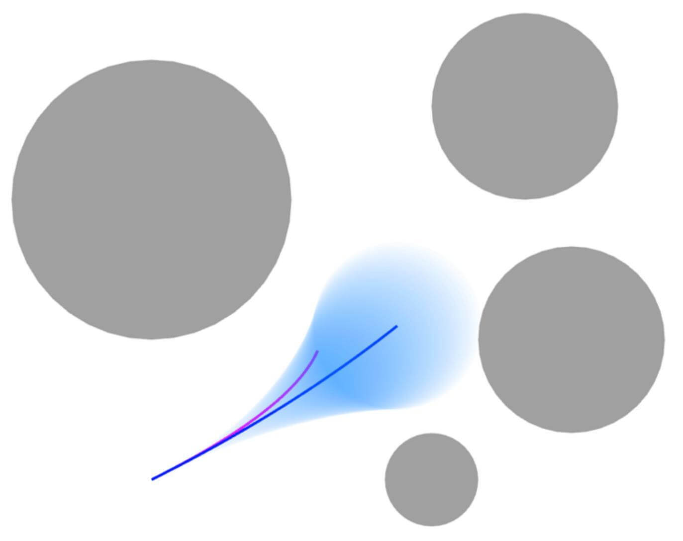
We set $n_{c}$ as 4, 5, 6 and test 5000 times for different scenarios $N_{o}$ $=1,2,3,4$ . qpOASES [30] is utilized as a QP solver, and the execution time to solve the QP problem is summarized in Table IV. As shown in the table, the computation time increases as the number of segments and obstacles increases. To satisfy real-time criteria (10 Hz) even as $N_{o}$ increases, we reduce $r_{q}(t)$ by defining $N_{\epsilon}$ furthest primitives as outliers, removing them from $\mathcal{P}_{s}$ , and recalculating $\mathcal{R}_{\textbf{q}}(t)$ . We determine the number of outliers $N_{\epsilon}=\epsilon_{p}|\mathcal{P}_{s}|$ with a factor $\epsilon_{p}$ . The effect of $\epsilon_{p}$ is visualized in Fig. 4(d), and it can lower the number of segments $M$ . With this strategy, real-time planning is possible even in complex and dense environments.

VI-F2 Benchmark test

We now demonstrate the proposed trajectory planner’s capability to maintain the target visibility against dynamic obstacles. The advantages of the proposed planner are analyzed by comparing it with non-convex optimization-based planners: [3], [5], and [13]. We consider a scenario where the target is static and a dynamic obstacle cuts in between the target and the drone. The total duration of the scenario is 10 seconds, and the position and velocity of the obstacle are updated every 20 milliseconds. We set $n_{c}$ as 5 and the planning horizon as 1.5 seconds for all planners. Fig. 9 visualizes the history of the positions of the target, the drone, and the obstacles, and Table V summarizes the performance indices related to jerkiness, collisions, and occlusions.

All other planners fail to avoid occlusion and collision because constraint violations can occur to some degree in non-convex optimization. In contrast, our planner considers future obstacle movements and successfully finds trajectories by treating the drone’s safety and the target visibility as hard constraints in a single QP. In addition, the computation efficiency of our method is an order of magnitude greater than other methods.

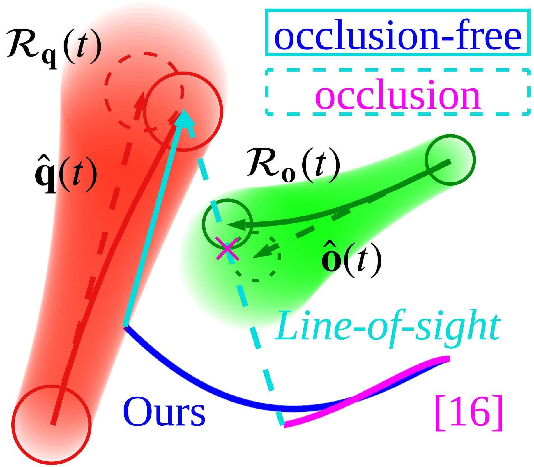
We also compare our planner with a motion-primitive-based planner [16] that does not account for the path prediction error. Fig. 10 illustrates a situation where occlusion may occur, highlighting that the success of planning can depend on whether the prediction error is considered. Even if the results of the planning method that does not consider the error are updated quickly, occlusion can still occur if the error accumulates. In contrast, our planner generates relatively large movements, which are suitable for maintaining the target visibility when obstacles approach.

VI-F3 Critical analysis

We now study the harsh situations that can fail to maintain the target visibility. The optimization cannot be solved for the following reasons: 1) conflicts between the target visibility constraints and actuator limit constraints and 2) incompatibility among the target visibility constraints. For example, when a dynamic obstacle cuts in between the target and the drone at high speed, the huge variation in the TVR over time conflicts with the actuator limits. Next, a situation where two dynamic obstacles cut in simultaneously from opposite directions may incur conflicts between the target visibility constraints. These obstacles force the drone to move in opposite directions. Target occlusion inevitably occurs when the target and obstacles align. In these cases, we formulate the optimization problem considering constraints, excluding the target visibility constraint. While occlusion may occur, drone safety is the top priority, and planning considering the target visibility resumes once conditions return to normal.

VII Chasing Scenario Validation

In this section, the presented method is validated through realistic simulators and real-world experiments.

VII-A Implementation Details

We perform AirSim [31] simulations for a benchmark test of our method with [16] and [17]. In real-world experiments, we install two ZED2 cameras facing opposite directions. The front-view camera is used for object detection and tracking, while the rear-view camera is used for the localization of the robot. Since the rear-view camera does not capture multiple moving objects in the camera image, the localization system is free from visual interference caused by dynamic objects, thereby preventing degradation in localization performance. Additionally, we utilize 3D human pose estimation to determine the positions of the humans. The humans in experiments are distinguished by color as described in [17]. By using depth information and an algorithm from [32], we build a static map. To distribute the computational burden, we use the Jetson Xavier NX to process data from the ZED2 cameras and the Intel NUC to build maps and run the QP-Chaser algorithm. To manage the payload on the drone, we utilize a coaxial octocopter and deploy Pixhawk4 as the flight controller. For consistent acquisition of positional and scale data of the target and the interrupter, the drone looks between them, and it adjusts its altitude to the height of the target. The parameters used in validations are summarized in Table VI. Since the pipeline is updated at short intervals, the time horizon $T$ is set to 1.5 seconds, which is relatively short. The desired distance, $r_{d}$ , is set to 4 meters for the ZED2 camera setup to ensure a visually pleasing capture of the target. Additionally, we set the screen ratio, $\gamma_{c}$ , to 1 to pursue the rule of thirds in cinematography.

VII-B Evaluation Metrics

TABLE VI: Problem Settings

Scenario Settings
Name	Single Target	Dual Target
drone radius ( $r_{c}$ ) [m]	0.4	0.4
camera FOV $(\theta_{f})$ $[{}^{\circ}]$	120	120
Prediction Parameters
Name	Single Target	Dual Target
time horizon ( $T$ ) [s]	1.5	1.5
$\#$ sampled points ( $N_{samp}$ )	2000	2000
Planning Parameters
Name	Single Target	Dual Target
polynomial degree $(n_{c})$	6	6
max velocity ( $v_{\text{max}}$ ) [m/s]	4.0	4.0
max acceleration ( $a_{\text{max}}$ ) [ $\text{m}/\text{s}^{2}$ ]	5.0	5.0
shooting distance ( $r_{d}$ ) [m]	$4.0$	$\cdot$
screen ratio ( $\gamma_{c}$ )	$\cdot$	1.0
tracking weight ( $w_{e}$ )	10.0	10.0
jerk weight ( $w_{j}$ )	0.01	0.01

In the validations, we evaluate the performance of the proposed planner using the following metrics: drone safety and target visibility. We measure the distances between the drone and targets, the minimum distance between the drone and obstacles, and the visibility score defined as follows:


		$\displaystyle\chi_{1}(t):=\\|{}_{\textbf{q}}\textbf{p}_{c}(t)\\|_{2}-r_{c}-r_{q}$		(42a)
		$\displaystyle\chi_{2}(t):=\underset{j:\mathcal{O}_{j}\in\mathcal{O}}{\min}\\|{}_{\textbf{o}_{j}}\textbf{p}_{c}(t)\\|_{2}-r_{o_{j}}-r_{c}$		(42b)
		$\displaystyle\psi_{1}(t):=\underset{j:\mathcal{O}_{j}\in\mathcal{O}}{\min}\psi(\textbf{p}_{c}(t);\textbf{q}(t),\mathcal{O}_{j})$		(42c)

Also, we assess the tracking performance in the image plane. First, we measure multi-object tracking accuracy (MOTA) and IDF1 to evaluate tracking accuracy. Then, we measure the visibility proportion, which is defined as follows:

\psi_{2}(t):=\begin{cases}1-\frac{b_{q}(t)\cap b_{o}(t)}{b_{q}(t)}\ (\text{if}\ \|{}_{\textbf{q}}\textbf{p}_{c}(t)\|_{2}\geq\|{}_{\textbf{o}}\textbf{p}_{c}(t)\|_{2})\\ 1\quad\ \ \qquad\qquad\text{(otherwise)}\end{cases}

(43)

where $b_{q}(t)$ and $b_{o}(t)$ represent the bounding boxes of the targets and obstacles in the camera image, respectively. The score $\psi_{2}(t)$ means the proportion of the unoccluded part of the targets’ bounding box. In the dual-target chasing scenarios, one target can be an obstacle occluding the other target, and the above metrics are measured accordingly. Throughout all validations, we use YOLO11 [33] for the object tracking.

TABLE VII: Comparison Between the Proposed Planner and Baselines (Simulation)

Metrics	Planner	Single Target		Dual Target
Metrics	Planner	Scenario 1	Scenario 2	Scenario 3	Scenario 4
Target Distance (42a) [m] $(\dagger)$	proposed	1.595/3.726	0.995/2.562	1.213/2.204	1.505/3.135
Target Distance (42a) [m] $(\dagger)$	baseline	1.198/3.298	-0.131/3.280	1.060/3.610	0.890/2.611
Obstacle Distance (42b) [m] $(\dagger)$	proposed	0.872/4.070	0.714/3.320	0.428/1.873	0.315/2.847
Obstacle Distance (42b) [m] $(\dagger)$	baseline	-0.264/1.715	-0.364/2.520	0.302/1.901	0.059/3.207
Visibility Score (42c) [m] $(\dagger)$	proposed	0.687/2.369	0.028/2.529	0.193/1.187	0.151/1.975
Visibility Score (42c) [m] $(\dagger)$	baseline	-0.397/1.183	-0.379/1.649	-0.260/0.834	-0.214/2.103
MOTA $(\uparrow)$	proposed	0.987	0.917	0.913	0.934
MOTA $(\uparrow)$	baseline	0.939	0.808	0.882	0.879
IDF1 $(\uparrow)$	proposed	0.994	0.990	0.997	0.997
IDF1 $(\uparrow)$	baseline	0.969	0.894	0.974	0.972
Visibility Proportion (43) $(\uparrow)$	proposed	1.0/1.0	0.523/0.996	0.726/0.998	0.951/0.999
Visibility Proportion (43) $(\uparrow)$	baseline	0.0/0.954	0.0/0.926	0.0/0.942	0.0/0.951
Computation Time [ms]	proposed	13.64	15.41	20.53	21.22
Computation Time [ms]	baseline	29.45	32.12	79.61	81.37

The upper and lower data in each metric represent the reported metrics of the proposed planner and the baselines (single target: [16], dual target: [17]), respectively. The values for the first, second, third, and sixth metrics indicate the (minimum/mean) performance. $\dagger$ means that a value below 0 indicates a collision or occlusion. $\uparrow$ means that higher is better.

VII-C Simulations

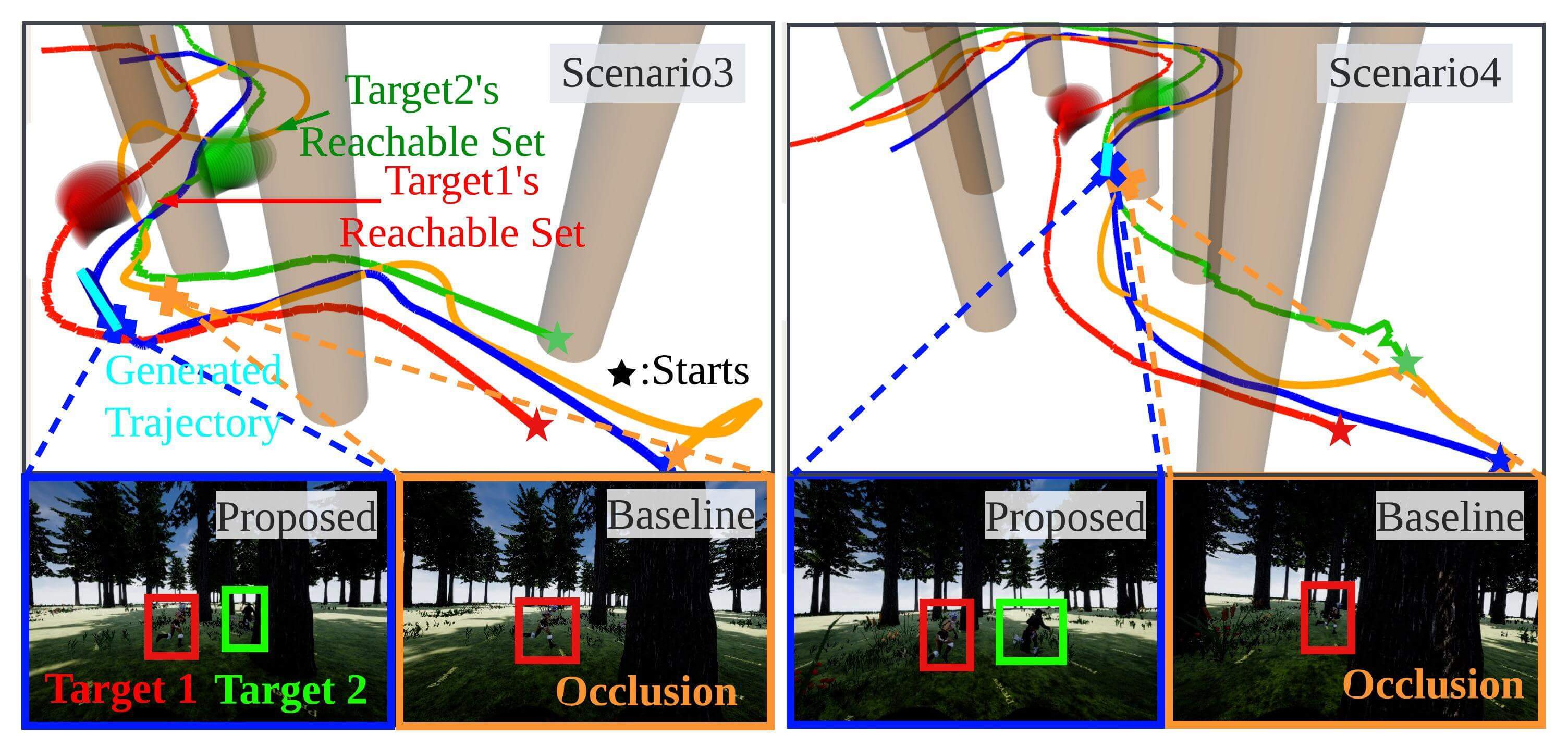
We test the proposed planner in scenarios where two actors run in the forest. To show the robust performance of the planner, we bring the following four scenarios. In the first two scenarios, one actor is the target and the other is the interrupter. In the remaining two scenarios, both actors are targets.

•

Scenario 1: The interrupter runs around the target, ceaselessly disrupting the shooting.
•

Scenario 2: The interrupter intermittently cuts in between the target and the drone.
•

Scenario 3: The two targets run while maintaining a short distance between them.
•

Scenario 4: The two targets run while varying the distance between them.

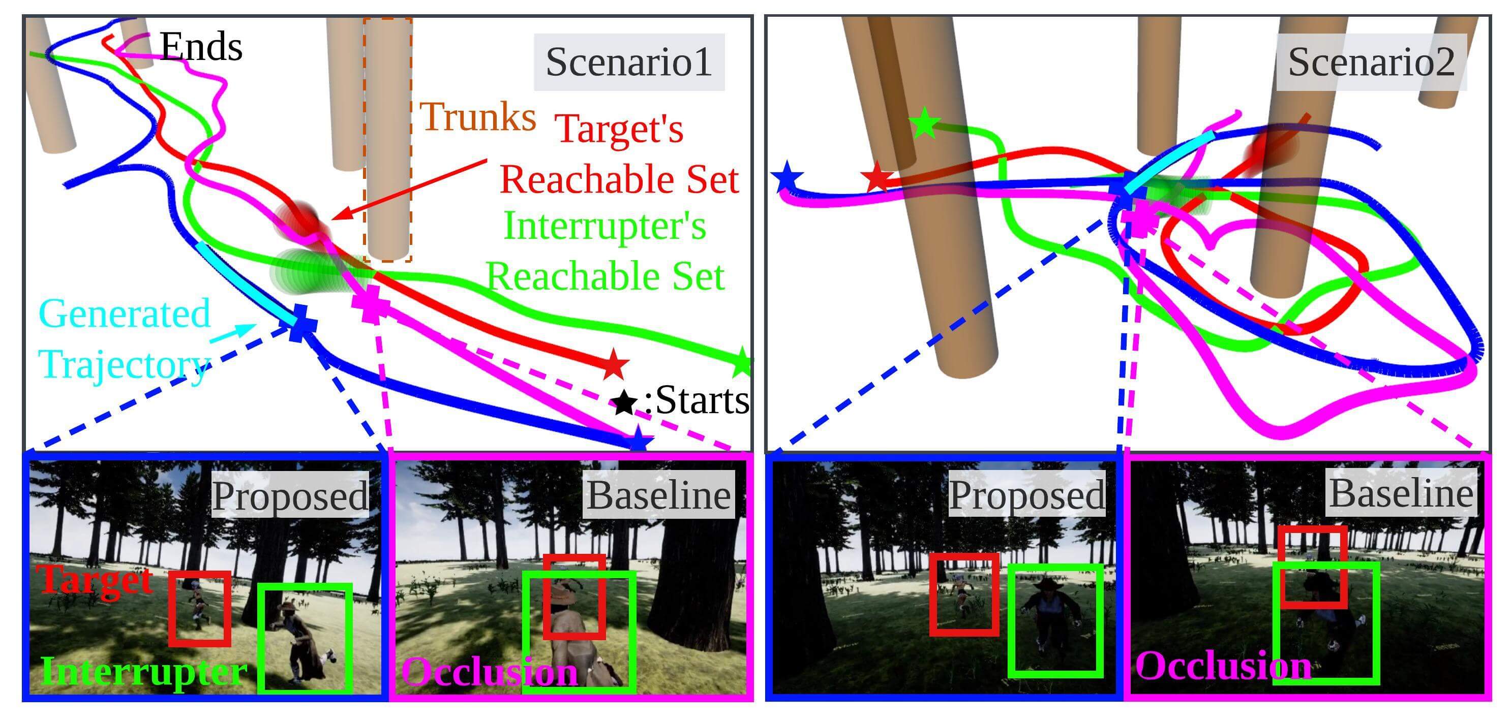
Of the many flight tests, we extract and report some of the 30-40 seconds long flights. We compare the proposed planner with the other state-of-the-art planners [16] in single-target chasing scenarios and [17] in dual-target chasing scenarios. Figs. 11 and 12 show the comparative results with key snapshots, and Table VII shows that the proposed approach makes the drone follow the target while maintaining the target visibility safely, whereas the baselines cause collisions and occlusions. There are rare cases in which partial occlusion occurs with our planner due to the limitations of the PD controller provided by the Airsim simulator. However, in the same situation, full occlusions occur with the baselines.

In single-target scenarios, [16] fails because it alters the chasing path topology when obstacles are close to the drone. In dual-target scenarios, [17] calculates good viewpoints considering the visibility score (42c) and camera FOV, but the path between these viewpoints does not guarantee the target visibility. In contrast, our planner succeeds in chasing because we consider these factors as hard constraints. Moreover, despite the heavy computational demands of the physics engine, the planning pipeline is executed within 25 milliseconds, which is faster than the baselines.

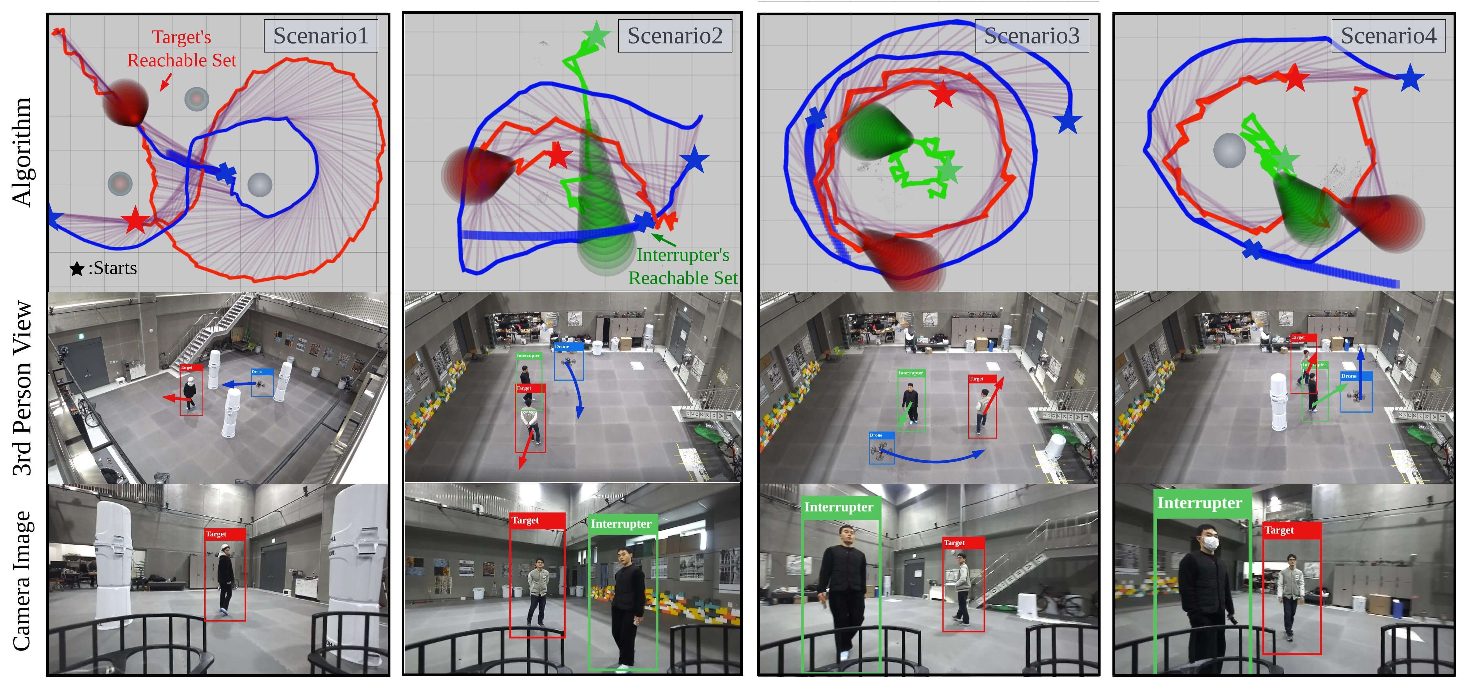
VII-D Experiments

To validate our chasing strategy, we conduct real-world experiments with several single- and dual-target tracking scenarios. Two actors move in an $8\times 11$ [m²] indoor space with stacked bins. As in the simulations, one actor is the target, and the other is the interrupter in single-target scenarios, while the two actors are both targets in dual-target scenarios.
For the single-target chasing, we bring the following scenarios.

•

Scenario S1: The drone senses the bins as static obstacles and follows the target.
•

Scenario S2: The target moves away from the drone, and the interrupter cuts in between the target and the drone.
•

Scenario S3: Two actors rotate in a circular way, causing the target to move away from the drone, while the interrupter consistently disrupts the visibility of the target.
•

Scenario S4: The interrupter intentionally hides behind bins and appears abruptly to obstruct the target.

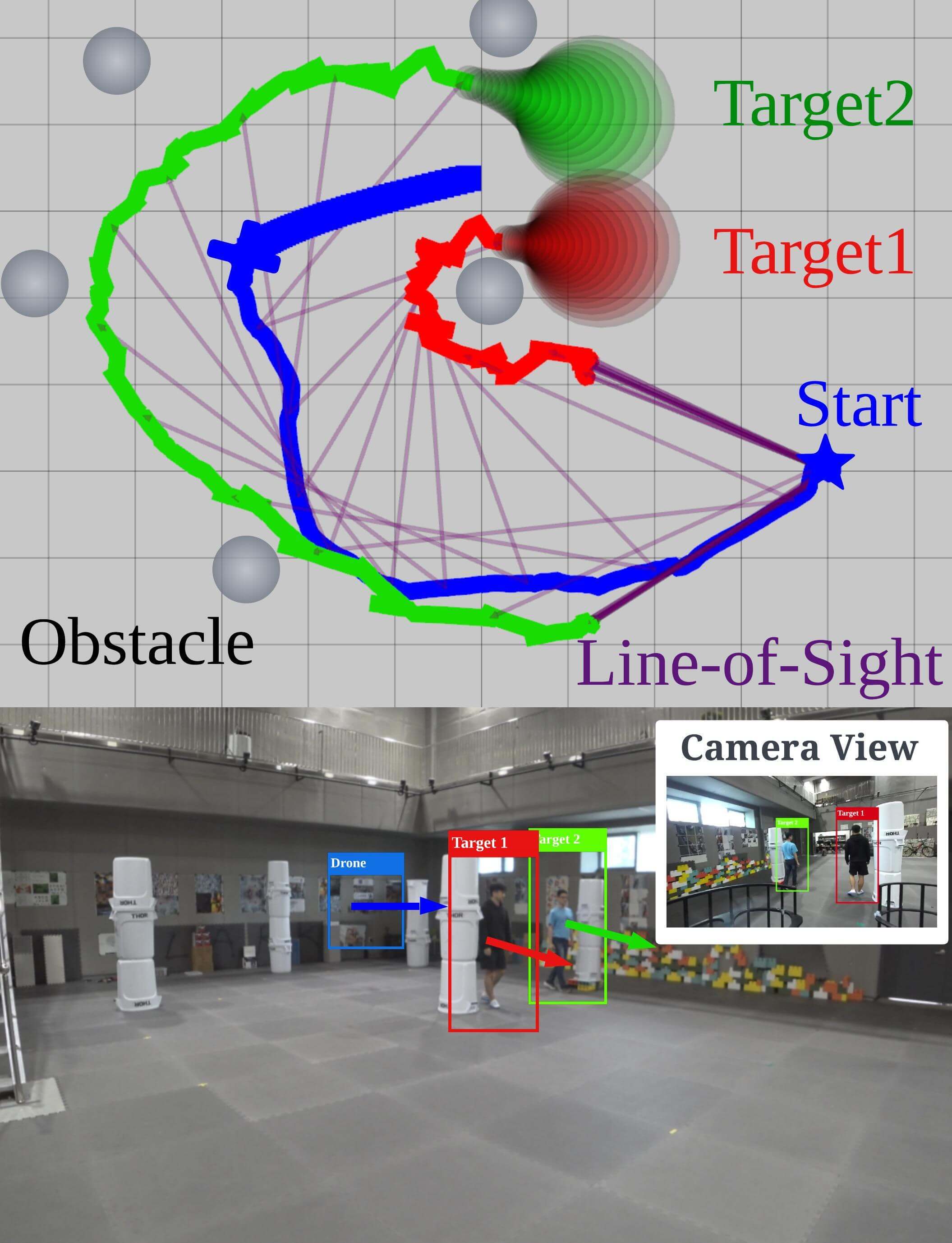
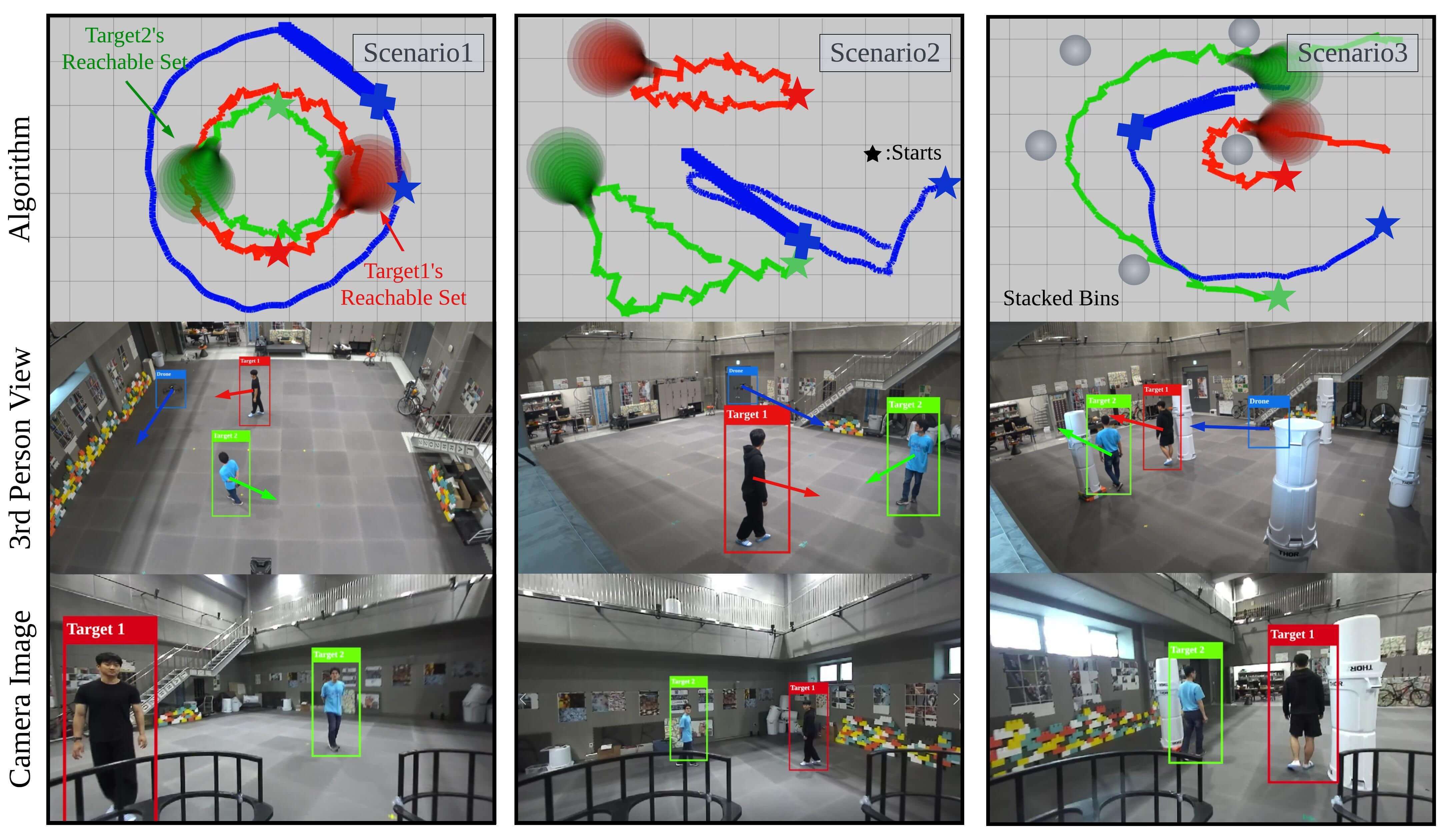
For the dual-target chasing, we bring the following scenarios.

•

Scenario D1: The targets move in a circular pattern. To capture both targets in the camera view, the drone also moves in circles.
•

Scenario D2: The targets move while repeatedly increasing and reducing their relative distance. The drone adjusts its distance from the targets to keep them within the image.
•

Scenario D3: The drone detects the bins and follows the targets among them.

Figs. 13 and 14 show the histories with key snapshots of the single- and dual-target experiments, respectively. The planner generates chasing trajectories in response to the targets’ diverse movements and obstacles’ interference. Table VIII confirms that the drone successfully followed the targets without collision and occlusion.

TABLE VIII: Reported Performance in Experiments

Metrics	Single Target				Dual Target
Metrics	Scenario S1	Scenario S2	Scenario S3	Scenario S4	Scenario D1	Scenario D2	Scenario D3
Target Distance (42a) [m] ( $\dagger$ )	1.668/2.303	1.301/2.153	1.793/2.382	0.805/1.739	1.336/2.037	1.061/3.349	1.567/2.358
Obstacle Distance (42b) [m] ( $\dagger$ )	0.534/2.289	0.701/2.285	1.405/2.109	0.545/1.862	2.316/2.877	1.094/3.277	0.209/1.889
Visibility Score (42c) [m] ( $\dagger$ )	0.393/2.111	1.020/1.678	1.302/1.831	0.765/1.461	2.403/2.809	1.397/3.099	0.534/2.289
MOTA ( $\uparrow$ )	0.998	0.990	0.987	0.990	0.991	0.844	0.990
IDF1 ( $\uparrow$ )	0.999	0.995	0.995	0.993	0.996	0.990	1.0
Visibility Proportion (43) ( $\uparrow$ )	1.0/1.0	1.0/1.0	1.0/1.0	1.0/1.0	1.0/1.0	1.0/1.0	0.901/0.995
Computation Time [ms]	12.61	14.63	16.12	15.32	14.61	13.94	20.81

The values for the first, second, third, and sixth metrics indicate the minimum/mean performance. $\dagger$ means that a value below 0 indicates a collision or occlusion. $\uparrow$ means that higher is better.

We use compressed RGB and depth images in the pipeline to record the camera images in limited onboard computer storage and to transfer images between computers. Since the compressed data is acquired at a slow rate, information about moving objects is updated slowly. Therefore, trajectories of moving objects drawn in Figs. 13 and 14 seem jerky. Nevertheless, the drone keeps the target visible and ensures its own safety by quickly updating the chasing trajectory.

VII-E Adaptability and Scalability

As shown in the validations, our planner can be used in environments such as forests or crowds, where obstacles can be modeled as cylinders. Extension to environments with ellipsoidal objects is manageable, but the QP-based approach that can handle unstructured obstacles should be studied further. Extension to multi-target chasing is also feasible. As in dual-target missions, we apply occlusion avoidance and FOV constraints to all pairs of targets, but the reference trajectory to keep high visibility of all targets needs further study.

VII-F Practicality

From a practical perspective, the proposed pipeline can be used in various applications, including the following:

•

Surveillance: tracking a suspicious person in crowds
•

Search and rescue: providing a missing person’s location in the forest until the rescue team arrives
•

Cinematography: producing smooth tracking shots of the main character in scenes with many background actors

In real-world experiments, we confirmed that despite the path prediction error, the drone successfully tracked the targets by quickly updating its chasing trajectory. However, to handle greater sensor noise and more severe unexpected target behaviors, not only is a fast planning algorithm required, but also greater maneuverability of the drone. Two cameras used for stable localization and two onboard computers to meet the pipeline’s real-time constraints significantly increase the overall weight of our system. Reducing the drone’s weight will be beneficial for its agility.

VIII Conclusion

We propose a real-time target-chasing planner among static and dynamic obstacles. First, we calculate the reachable sets of moving objects in obstacle environments using Bernstein polynomial primitives. Then, to prevent target occlusion, we define a continuous-time target-visible region (TVR) based on path homotopy while considering the camera field-of-view limit. The reference trajectory for target tracking is designed and utilized with TVR to formulate trajectory optimization as a single QP problem. The proposed QP formulation can generate dynamically feasible, collision-free, and occlusion-free chasing trajectories in real-time. We extensively demonstrate the effectiveness of the proposed planner through challenging scenarios, including realistic simulations and indoor experiments. In the future, we plan to extend our work to chase multiple targets in environments with moving unstructured obstacles.

Appendix A Implementation of Collision Check

The collision between the trajectories of the moving object and the $j$ -th obstacle in (12) can be determined using coefficients of Bernstein polynomials.

		$\displaystyle\\|\hat{\textbf{p}}_{i}(t)-\textbf{o}_{j}(t)\\|_{2}^{2}-(r_{p0}+r_{o_{j}}(t))^{2}\geq 0\Longleftrightarrow$		(44)
		$\displaystyle\sum_{k=0}^{2n_{p}}\begin{pmatrix}2n_{p}\\ k\end{pmatrix}^{-1}{}^{ij}C_{k}b_{k,2n_{p}}(t,0,T)\geq 0,\ {}^{\forall}j\in\{1,\ldots,\|\mathcal{O}\|\},$
		where
		$\displaystyle{}^{ij}C_{k}\ =\sum_{l=\max(0,k-n_{p})}^{\min(k,n_{p})}\begin{pmatrix}n_{p}\\ l\end{pmatrix}\begin{pmatrix}n_{p}\\ k-l\end{pmatrix}\Big{(}{}^{ij}_{o}\textbf{p}_{(x)}[l]\ {}^{ij}_{o}\textbf{p}_{(x)}[k-l]$
		$\displaystyle\quad\quad\quad\quad\quad\quad\quad+{}^{ij}_{o}\textbf{p}_{(y)}[l]\ {}^{ij}_{o}\textbf{p}_{(y)}[k-l]-{}^{ij}_{o}\textbf{r}[l]\ {}^{ij}_{o}\textbf{r}[k-l]\Big{)},$
		$\displaystyle{}^{ij}_{o}\textbf{p}_{(x)}=\textbf{p}_{i(x)}-\textbf{o}_{j(x)},{}^{ij}_{o}\textbf{p}_{(y)}=\textbf{p}_{i(y)}-\textbf{o}_{j(y)},{}^{ij}_{o}\textbf{r}=\textbf{r}_{o_{j}}+r_{p0}$

$[l]$ represents $l$ -th elements of a vector, and $\textbf{r}_{o_{j}}$ is the Bernstein coefficient representing the radius of the $j$ -th obstacle. The condition ${}^{ij}C_{k}\geq 0,\ k=0,\ldots,2n_{p}$ makes the moving objects not collide with obstacles during $[0,T]$ .

Appendix B Proof of the Proposition1

Motion primitives for object prediction derived from (9) are represented as follows.

		$\displaystyle\hat{\textbf{p}}_{i}(t)=\textbf{P}_{i,n_{p}}^{\top}\textbf{b}_{n_{p}}(t,T)$		(45)
		$\displaystyle\text{where}\ \textbf{P}_{i,n_{p}}=U_{3,n_{p}}^{\top}\textbf{P}_{i,3}^{*},$
		$\displaystyle\textbf{P}_{3}^{*}=[\hat{\textbf{p}}_{0},\hat{\textbf{p}}_{0}+\frac{1}{3}\hat{\textbf{p}}_{0}^{\prime}T,\frac{2}{3}\hat{\textbf{p}}_{0}+\frac{1}{3}\textbf{s}_{p,i}+\frac{1}{3}\hat{\textbf{p}}_{0}^{\prime}T,\textbf{s}_{p,i}]^{\top},$
		$\displaystyle\textbf{b}_{n_{p}}(t,T)=[b_{0,n_{p}}(t,0,T),\ldots,b_{n_{p},n_{p}}(t,0,T)]^{\top},\ n_{p}\geq 3,$
		$\displaystyle U_{m,n}=\{u_{j,k}\}\in\mathbb{R}^{(n+1)\times(m+1)},\ m\geq n,$
		$\displaystyle u_{j,j+k}=\frac{\begin{pmatrix}n\\ j\end{pmatrix}\begin{pmatrix}m-n\\ k\end{pmatrix}}{\begin{pmatrix}m\\ j+k\end{pmatrix}}$

The difference between $\hat{\textbf{p}}_{i}(t)$ and $\hat{\textbf{p}}_{j}(t)$ , $\|\hat{\textbf{p}}_{i}(t)-\hat{\textbf{p}}_{j}(t)\|=\|\textbf{s}_{p,i}-\textbf{s}_{p,j}\|\frac{t^{2}}{T^{2}}$ . Therefore, in order to minimize distance sum in (14), it is sufficient to investigate sampled endpoints $\textbf{s}_{p,i}$ .

Appendix C TVR Formulation

We derive TVR-O, which are represented as (18) and (19), and TVR-F, which are represented as (24). For the mathematical simplicity, we omit time $t$ to represent variables.

C-A TVR-O Formulation

As mentioned in Section. VI-B, there are two cases where the reachable sets of the target and obstacles Case 1: do not overlap and Case 2: overlap.

C-A1 Case 1: Non-overlap

Fig. 15(a) shows the TVR-O, when the relation between the target, the obstacle, and the drone corresponds to Class O1. TVR-O is made by the tangential line, and its normal vector is represented as $\textbf{n}_{qo}$ . TVR-O is represented as follows:

\textbf{n}_{qo}^{\top}(\textbf{x}-\hat{\textbf{o}})\geq r_{o}

(46)

$\textbf{n}_{qo}$ is perpendicular to the tangential line, and the line is rotated by $\theta_{qo}$ from a segment connecting the centers of the reachable sets. By using rotation matrices, $\textbf{n}_{qo}$ becomes as follows.


	$\displaystyle\textbf{n}_{qo}=\begin{bmatrix}0&1\\ -1&0\end{bmatrix}\begin{bmatrix}\cos\theta_{q0}&-\sin\theta_{qo}\\ \sin\theta_{qo}&\cos\theta_{q0}\end{bmatrix}\frac{\hat{\textbf{q}}-\hat{\textbf{o}}}{\\|\hat{\textbf{q}}-\hat{\textbf{o}}\\|}$		(47a)
	$\displaystyle\sin\theta_{qo}=\frac{r_{q}+r_{o}}{\\|\hat{\textbf{q}}-\hat{\textbf{o}}\\|},\ \cos\theta_{qo}=\sqrt{1-\sin^{2}\theta_{qo}}$		(47b)

By multiplying $\|\hat{\textbf{q}}-\hat{\textbf{o}}\|^{2}_{2}$ to (46), we can acquire (18).

C-A2 Case 2: Overlap

Fig. 15(b) shows the TVR-O, when the reachable sets overlap. TVR-O is made by the tangential line that is perpendicular to the segment connecting the centers of the reachable sets. TVR-O is represented as follows:


		$\displaystyle\textbf{n}_{qo}^{\top}(\textbf{x}-\hat{\textbf{q}})+r_{q}\geq 0,$		(48a)
		$\displaystyle\textbf{n}_{qo}=\frac{\hat{\textbf{q}}-\hat{\textbf{o}}}{\\|\hat{\textbf{q}}-\hat{\textbf{o}}\\|}$		(48b)

By multiplying $\|\hat{\textbf{q}}-\hat{\textbf{o}}\|$ to (48a), we can acquire (19).

C-B TVR-F Formulation

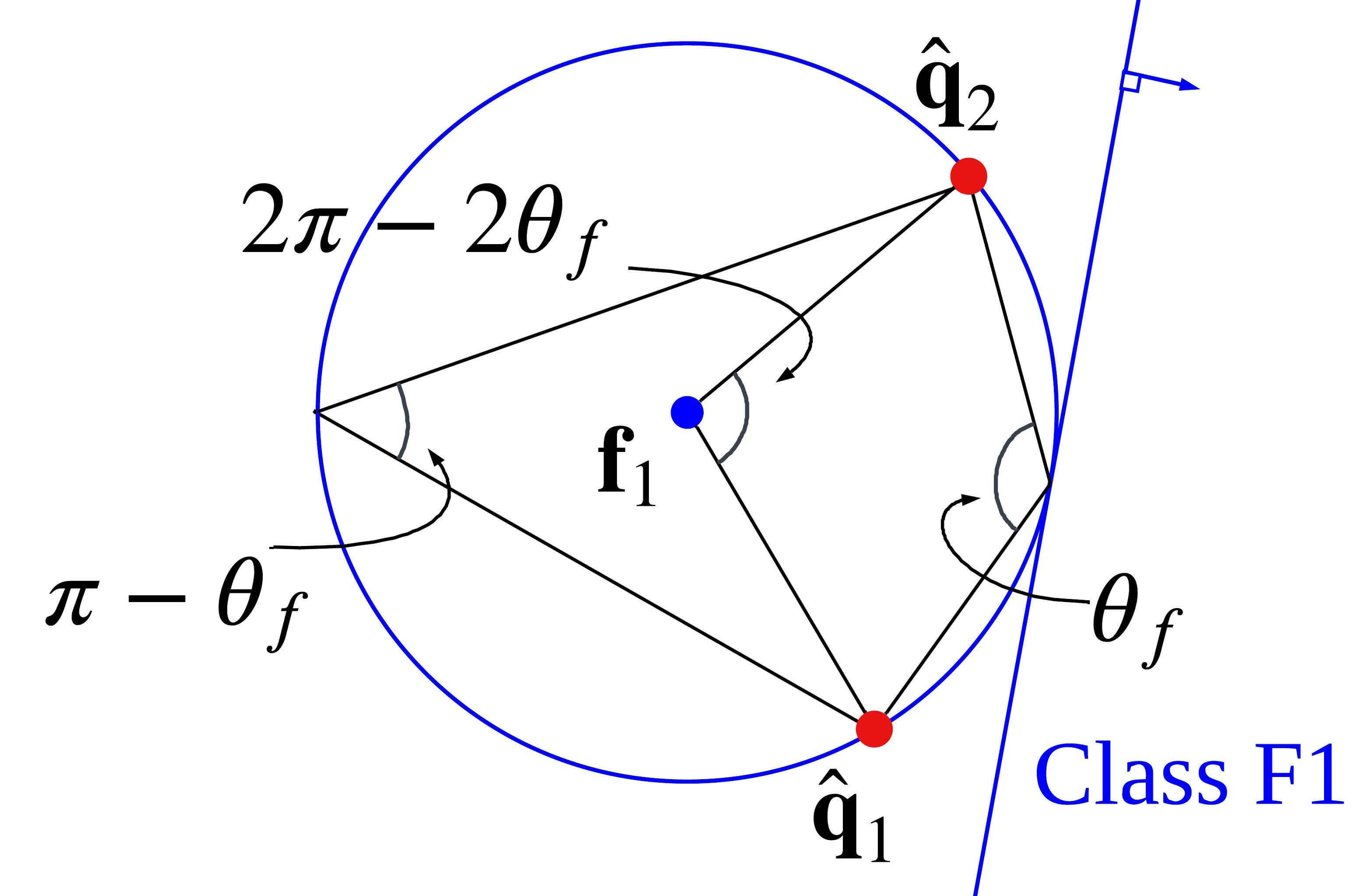
Fig. 16 shows the TVR-F, when the relation between the targets and the drone corresponds to Class F1. The blue circle has inscribed angles of an arc tracing two points at $\hat{\textbf{q}}_{1}$ and $\hat{\textbf{q}}_{2}$ equals camera FOV $\theta_{f}$ . The position of its center, $\textbf{f}_{1}$ , is obtained by a relation: rotation of the segment connecting $\textbf{f}_{1}$ and $\hat{\textbf{q}}_{1}$ by an angle $2\pi-2\theta_{f}$ becomes the segment connecting $\textbf{f}_{1}$ and $\hat{\textbf{q}}_{2}$ .

\begin{bmatrix}\cos(2\pi-2\theta_{f})&-\sin(2\pi-2\theta_{f})\\ \sin(2\pi-2\theta_{f})&\cos(2\pi-2\theta_{f})\end{bmatrix}(\hat{\textbf{q}}_{1}-\textbf{f}_{1})=\hat{\textbf{q}}_{2}-\textbf{f}_{1}

(49)

The angle $2\pi-2\theta_{f}$ comes from the property of the inscribed angle. The radius of the circle. $r_{f}$ , is equal to the distance between the points at $\hat{\textbf{q}}_{1}$ and $\textbf{f}_{1}$ .

	$\displaystyle r_{f}$	$\displaystyle=\\|\textbf{f}_{1}-\hat{\textbf{q}}_{1}\\|=\frac{1}{2}\bigg{\\|}\begin{bmatrix}1&\cot{\theta_{f}}\\ -\cot{\theta_{f}}&1\end{bmatrix}(\hat{\textbf{q}}_{2}-\hat{\textbf{q}}_{1})\bigg{\\|}$		(50)
		$\displaystyle=\frac{1}{2\sin{\theta_{f}}}\\|{}_{\hat{\textbf{q}}_{1}}\hat{\textbf{q}}_{2}\\|$		(50)

TVR-F is made by the tangential line that is parallel to the segments connecting the two targets, and is represented as follows:

(\textbf{x}-\textbf{f}_{1})^{\top}\begin{bmatrix}0&1\\ -1&0\end{bmatrix}\frac{\hat{\textbf{q}}_{2}-\hat{\textbf{q}}_{1}}{\|\hat{\textbf{q}}_{2}-\textbf{q}_{1}\|}\geq r_{f}

(51)

By substituting $\textbf{f}_{1}$ and $r_{f}$ in (51) with terms represented by $\hat{\textbf{q}}_{1}$ and $\hat{\textbf{q}}_{2}$ , we can acquire (24).

References

[1] M. Aranda, G. López-Nicolás, C. Sagüés, and Y. Mezouar, “Formation control of mobile robots using multiple aerial cameras,” IEEE Transactions on Robotics, vol. 31, no. 4, pp. 1064–1071, 2015.
[2] A. Alcántara, J. Capitán, R. Cunha, and A. Ollero, “Optimal trajectory planning for cinematography with multiple unmanned aerial vehicles,” Robotics and Autonomous Systems, vol. 140, p. 103778, 2021.
[3] B. Penin, P. R. Giordano, and F. Chaumette, “Vision-based reactive planning for aggressive target tracking while avoiding collisions and occlusions,” IEEE Robotics and Automation Letters, vol. 3, no. 4, pp. 3725–3732, 2018.
[4] H. Huang, A. V. Savkin, and W. Ni, “Online uav trajectory planning for covert video surveillance of mobile targets,” IEEE Transactions on Automation Science and Engineering, vol. 19, no. 2, pp. 735–746, 2022.
[5] R. Bonatti, W. Wang, C. Ho, A. Ahuja, M. Gschwindt, E. Camci, E. Kayacan, S. Choudhury, and S. Scherer, “Autonomous aerial cinematography in unstructured environments with learned artistic decision‐making,” Journal of Field Robotics, vol. 37, no. 4, pp. 606 – 641, June 2020.
[6] H. Wang, X. Zhang, Y. Liu, X. Zhang, and Y. Zhuang, “Svpto: Safe visibility-guided perception-aware trajectory optimization for aerial tracking,” IEEE Transactions on Industrial Electronics, vol. 71, no. 3, pp. 2716–2725, 2024.
[7] J. Ji, N. Pan, C. Xu, and F. Gao, “Elastic tracker: A spatio-temporal trajectory planner flexible aerial tracking,” ArXiv, vol. abs/2109.07111, 2021.
[8] Z. Zhang, Y. Zhong, J. Guo, Q. Wang, C. Xu, and F. Gao, “Auto filmer: Autonomous aerial videography under human interaction,” IEEE Robotics and Automation Letters, vol. 8, no. 2, pp. 784–791, 2023.
[9] Z. Han, R. Zhang, N. Pan, C. Xu, and F. Gao, “Fast-tracker: A robust aerial system for tracking agile target in cluttered environments,” in 2021 IEEE International Conference on Robotics and Automation (ICRA), 2021, pp. 328–334.
[10] N. Pan, R. Zhang, T. Yang, C. Cui, C. Xu, and F. Gao, “Fast‐tracker 2.0: Improving autonomy of aerial tracking with active vision and human location regression,” IET Cyber-Systems and Robotics, vol. 3, 11 2021.
[11] S. Cui, Y. Chen, and X. Li, “A robust and efficient uav path planning approach for tracking agile targets in complex environments,” Machines, vol. 10, no. 10, 2022. [Online]. Available: https://www.mdpi.com/2075-1702/10/10/931
[12] B. Jeon, Y. Lee, and H. J. Kim, “Integrated motion planner for real-time aerial videography with a drone in a dense environment,” in 2020 IEEE International Conference on Robotics and Automation (ICRA), 2020, pp. 1243–1249.
[13] T. Nägeli, J. Alonso-Mora, A. Domahidi, D. Rus, and O. Hilliges, “Real-time motion planning for aerial videography with dynamic obstacle avoidance and viewpoint optimization,” IEEE Robotics and Automation Letters, vol. 2, no. 3, pp. 1696–1703, 2017.
[14] H. Masnavi, J. Shrestha, M. Mishra, P. B. Sujit, K. Kruusamäe, and A. K. Singh, “Visibility-aware navigation with batch projection augmented cross-entropy method over a learned occlusion cost,” IEEE Robotics and Automation Letters, vol. 7, no. 4, pp. 9366–9373, 2022.
[15] H. Masnavi, V. K. Adajania, K. Kruusamäe, and A. K. Singh, “Real-time multi-convex model predictive control for occlusion-free target tracking with quadrotors,” IEEE Access, vol. 10, pp. 29 009–29 031, 2022.
[16] B. F. Jeon, C. Kim, H. Shin, and H. J. Kim, “Aerial chasing of a dynamic target in complex environments,” International Journal of Control, Automation, and Systems, vol. 20, no. 6, pp. 2032–2042, 2022.
[17] B. F. Jeon, Y. Lee, J. Choi, J. Park, and H. J. Kim, “Autonomous aerial dual-target following among obstacles,” IEEE Access, vol. 9, pp. 143 104–143 120, 2021.
[18] P. Pueyo, J. Dendarieta, E. Montijano, A. Murillo, and M. Schwager, “Cinempc: A fully autonomous drone cinematography system incorporating zoom, focus, pose, and scene composition,” IEEE Transactions on Robotics, vol. PP, pp. 1–18, 01 2024.
[19] N. R. Gans, G. Hu, K. Nagarajan, and W. E. Dixon, “Keeping multiple moving targets in the field of view of a mobile camera,” IEEE Transactions on Robotics, vol. 27, no. 4, pp. 822–828, 2011.
[20] M. Zarudzki, H.-S. Shin, and C.-H. Lee, “An image based visual servoing approach for multi-target tracking using an quad-tilt rotor uav,” in 2017 International Conference on Unmanned Aircraft Systems (ICUAS), 2017, pp. 781–790.
[21] J. Chen, T. Liu, and S. Shen, “Tracking a moving target in cluttered environments using a quadrotor,” in 2016 IEEE/RSJ International Conference on Intelligent Robots and Systems (IROS). IEEE, 2016, pp. 446–453.
[22] S. Bhattacharya, M. Likhachev, and V. Kumar, “Topological constraints in search-based robot path planning,” Autonomous Robots, vol. 33, 10 2012.
[23] J. R. Munkres, “Topology prentice hall,” Inc., Upper Saddle River, 2000.
[24] D. Mellinger and V. Kumar, “Minimum snap trajectory generation and control for quadrotors,” in 2011 IEEE International Conference on Robotics and Automation, 2011, pp. 2520–2525.
[25] L. F. L. et al, “Optimal and robust estimation: With an introduction to stochastic control theory, second edition,” CRC Press., 2008.
[26] G. Collins et al., “Fundamental numerical methods and data analysis,” Fundamental Numerical Methods and Data Analysis, by George Collins, II., 1990.
[27] A. Marco, J.-J. Martı et al., “A fast and accurate algorithm for solving bernstein–vandermonde linear systems,” Linear algebra and its applications, vol. 422, no. 2-3, pp. 616–628, 2007.
[28] B. F. Jeon and H. J. Kim, “Online trajectory generation of a mav for chasing a moving target in 3d dense environments,” in 2019 IEEE/RSJ International Conference on Intelligent Robots and Systems (IROS), 2019, pp. 1115–1121.
[29] C. Kielas-Jensen and V. Cichella, “Bebot: Bernstein polynomial toolkit for trajectory generation,” in 2019 IEEE/RSJ International Conference on Intelligent Robots and Systems (IROS), 2019, pp. 3288–3293.
[30] H. J. Ferreau, C. Kirches, A. Potschka, H. G. Bock, and M. Diehl, “qpoases: A parametric active-set algorithm for quadratic programming,” Mathematical Programming Computation, vol. 6, no. 4, pp. 327–363, 2014.
[31] S. Shah, D. Dey, C. Lovett, and A. Kapoor, “Airsim: High-fidelity visual and physical simulation for autonomous vehicles,” in Field and Service Robotics, 2017. [Online]. Available: https://arxiv.org/abs/1705.05065
[32] M. Przybyła, “Detection and tracking of 2d geometric obstacles from lrf data,” in 2017 11th International Workshop on Robot Motion and Control (RoMoCo). IEEE, 2017, pp. 135–141.
[33] G. Jocher and J. Qiu, “Ultralytics yolo11,” 2024. [Online]. Available: https://github.com/ultralytics/ultralytics