QM abelian varieties, hypergeometric character sums and modular forms

(Reference: [85]). A Fuchsian subgroup of the first kind is a discrete subgroup $\Gamma\subset\mathrm{SL}_{2}(\mathbf{R})$ such that the invariant volume $\Gamma\backslash\mathrm{SL}_{2}(\mathbf{R})$ is finite. This acts on the upper half-plane $\mathfrak{H}$ by

The upper half-plane is conformally equivalent to the open unit disk $\mathfrak{D}$, via the map $z\mapsto w=(z-i)/(z+i)$. This reflects the isomorphism $\mathrm{SU}(1,1)\cong\mathrm{SL}_{2}(\mathbf{R})$, where

There are isomorphisms $\mathrm{SL}_{2}(\mathbf{R})/\mathrm{SO}(2)\cong\mathfrak{H\cong}\mathfrak{D}$ where

For a Fuchsian subgroup $\Gamma$ of first kind, let $X_{\Gamma}^{an}=\Gamma\backslash\mathfrak{H}$ or $\Gamma\backslash\mathfrak{H}^{*}$ according to whether $\Gamma$ cocompact or not. Here $\mathfrak{H}^{*}$ is the union of $\mathfrak{H}$ and the cusps of $\Gamma$, if any. We have a finite set $S=S_{c}\cup S_{e}\subset X_{\Gamma}$ of points which are cusps or elliptic points, that is, their preimages in $\mathfrak{H}^{*}$ are cusps or elliptic points of $\Gamma$, respectively. Let

the complement of the set of cusps and elliptic points, and the complement of the set of cusps, respectively. Note that $p:\mathfrak{H}-\{\text{elliptic points of \ }\Gamma\}\to X_{\Gamma}^{\circ}$ is a covering space in the sense of topology. In particular, if $\Gamma$ has no elliptic points, then $p:\mathfrak{H}\to Y_{\Gamma}$ is the universal covering of $Y_{\Gamma}$. The action of $\Gamma$ on $\mathfrak{H}^{*}$ is via the quotient $\bar{\Gamma}$ in $\mathrm{PSL}_{2}(\mathbf{R})$. For the groups in this paper, $\bar{\Gamma}=\Gamma/\Gamma\cap\{\pm I\}$. Therefore, if $\Gamma$ torsion-free, then $p:\mathfrak{H}\to Y_{\Gamma}$ is the universal covering of $Y_{\Gamma}$, and the fundamental group at any base-point $x$

an isomorphism unique up to inner automorphism. In the quaternion cases this is $\pi_{1}(X_{\Gamma},x)\cong\Gamma$ for $\Gamma$ without torsion. In general, there is an epimorphism

If $\Gamma\subset\mathrm{SL}_{2}(\mathbf{R})$ is a Fuchsian subgroup of the first kind, and $k\geq 0$ is an integer, we recall that a modular form of weight $k$ is a holomorphic function $f(z)$ for $z\in\mathfrak{H}$ such that

which satisfies a growth condition at the cusps. For each cusp $c$ of $\Gamma$ there is a parameter $q_{c}$ such that a modular form has an expansion at $c$: $f=a_{0}+a_{1}q_{c}+a_{2}q_{c}^{2}+...$. A cusp form is one that vanishes at every cusp i.e., $a_{0}=0$ at every cusp of $\Gamma$. The space of cusp forms $S_{k}(\Gamma)$ is finite dimensional over $\mathbf{C}$. We assume the reader is familiar with the standard subgroups $\Gamma(N),\Gamma_{0}(N)\subset\mathrm{SL}_{2}(\mathbf{Z})$ as well as the Hecke operators $T(p)$ (the latter only defined in the case of arithmetically defined Fuchsian subgroups).

In our work, we consider those $\Gamma$ which are arithmetically defined subgroups. There are two cases:

• 1.

  Elliptic modular case. $\Gamma$ is commensurable with $\mathrm{SL}_{2}(\mathbf{Z})$. Then the cusps of $\Gamma$ is the set of rational numbers and the point $\infty$.

• 2.

  Quaternion case. $\Gamma$ is commensurable to the set $O_{B}^{1}$ of norm 1 elements in a maximal order $O_{B}$ of an indefinite quaternion algebra $B$ over $\mathbf{Q}$. That is, we choose once and for all an embedding $B\subset M_{2}(\mathbf{R})$, which induces an embedding $\theta:O_{B}^{1}\subset\mathrm{SL}_{2}(\mathbf{R})$. In this case, the set of cusps is empty, so $\mathfrak{H}^{*}=\mathfrak{H}$.

In both these cases, Shumura’s theory of canonical models shows that these Riemann surfaces are the $\mathbf{C}$-points of an algebraic curve, denoted $X_{\Gamma}$ defined over a number field $k_{\Gamma}$. We will use the notation $X_{\Gamma}$ for the corresponding Riemann surface, if there is no ambiguity. If necessary, we use $X^{an}_{\Gamma}$ to denote the analytic space.

These curves are (in general coarse) moduli spaces. If $\Gamma$ has no torsion, then there are universal families of abelian varieties $f:A_{\Gamma}\to Y_{\Gamma}$ with additional structures. In the elliptic modular cases these are families of elliptic curves $f:E_{\Gamma}\to Y_{\Gamma}$. In the quaternion cases, $Y_{\Gamma}=X_{\Gamma}$, these are families of 2-dimensional abelian varieties with an action of the quaternion algebra, that is, with a homomorphism

and additional structure.

The quaternion case with $D=6$ will be discussed in detail in section 7.

In this work, we consider those $\Gamma$ that are (or are closely related to) triangle groups. We recall the definition: Let $a,b,c\in\mathbf{Z}_{\geq 2}\cup\{\infty\}$, with $a\leq b\leq c$. Define

and refer to $(a,b,c)$ as spherical, Euclidean, hyperbolic, depending on whether $\chi(a,b,c)$ is $>0$, $=0$ or $<0$ respectively. In each of these three cases we associate a geometry

Spherical triples: $(2,3,3)$, $(2,3,4)$, $(2,3,5)$, $(2,2,c)$, for $c\geq 2$. Euclidean triples: $(2,2,\infty)$, $(2,3,6)$, $(2,4,4)$, $(3,3,3)$. The rest are hyperbolic. Among them, there are finitely many arithmetic triangle groups, which were enumerated by Takeuchi, see [89], [90]. To each triple we have the associated triangle group, defined as

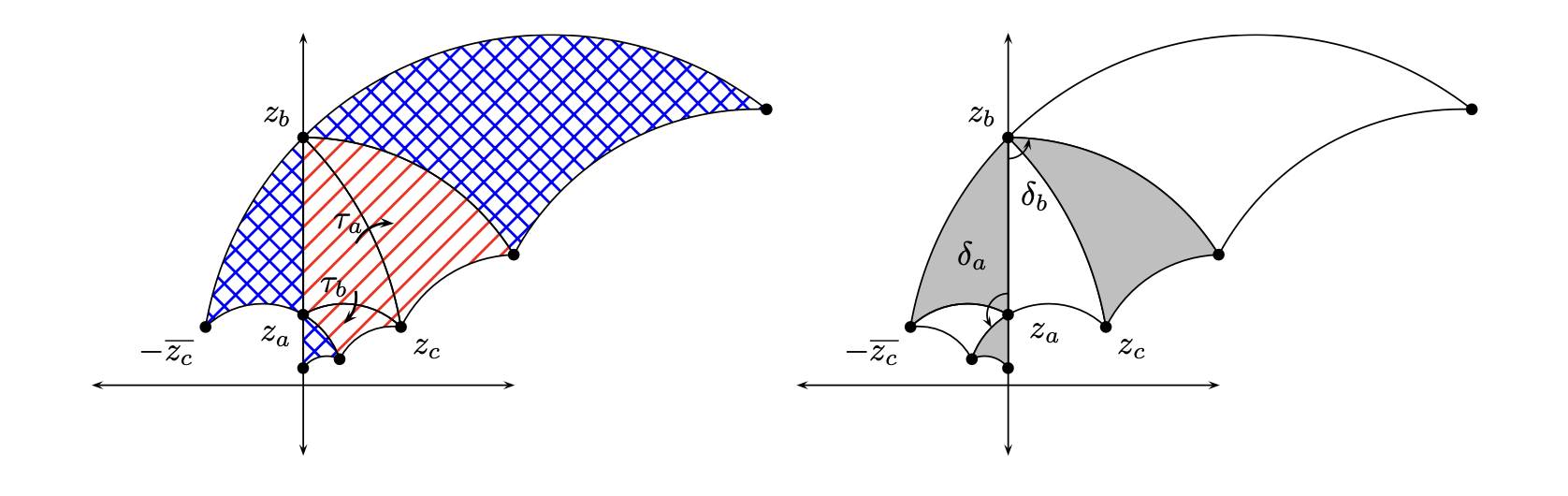
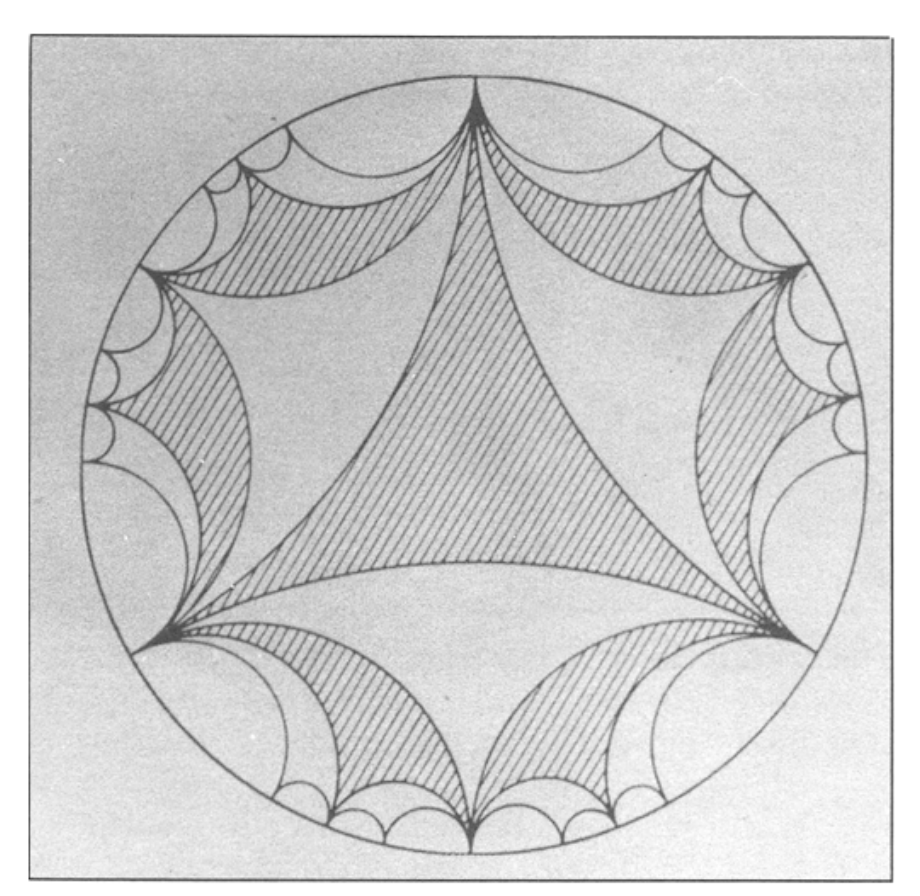
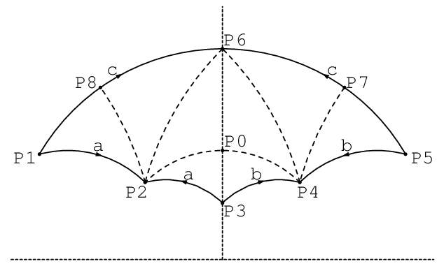
We have representation of $\Delta(a,b,c)$ via isometries of the associated geometry $H$ as follows. Let $T$ be a geodesic triangle in $H$ with angles $\pi/a,\pi/b,\pi/c$. Let $\tau_{a}$, $\tau_{b}$, $\tau_{c}$ be reflections in the three sides of $T$. The group generated by $\tau_{a},\tau_{b},\tau_{c}$ is a discrete group with fundamental domain $T$. The subgroup of orientation-preserving isometries is generated by

satisfies the relations of $\Delta(a,b,c)$ with $\delta_{p}$ a counterclockwise rotation at the vertex with angle $2\pi i/p$. The quotient space $X(\Delta(a,b,c)):=\Delta(a,b,c)\backslash H$ is a Riemann orbifold of genus zero. The fundamental domain $D_{\Delta}$ is then a union of $T$ and a reflected image of $T$.

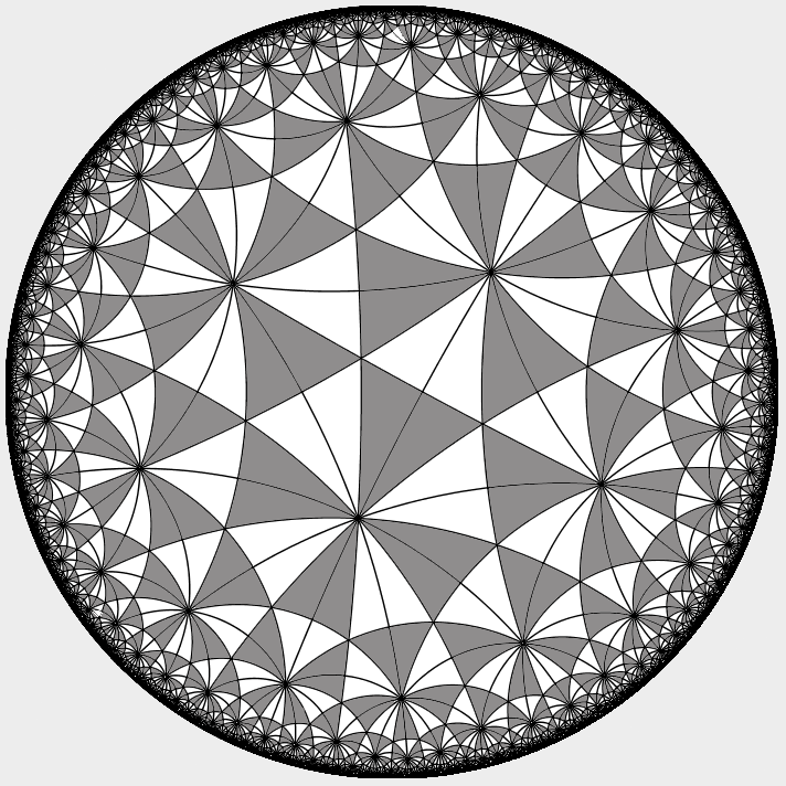
The relevance of triangle groups for hypergeometric equations arises from the fundamental theorem of H. A. Schwarz [80]. Given two independent solutions $y_{1}$ and $y_{2}$ to a hypergeometric differential equation, the ratio $\eta=y_{1}/y_{2}$ maps the complex upper half-plane conformally onto a region $T$ in the extended complex plane which is bounded by circular arcs. For the function

the angles are $p\pi$, $q\pi$, $r\pi$ where $p=|1-c|$, $q=|c-a-b|$, $r=|a-b|$. Schwarz observed that the monodromy of the differential equation gave rise to isometries of the associated geometry $H$. In some cases, one obtains by analytic continuation a tessellation of $H$. For this to extend to a tesselation we must have that $p,p,r$ are all in the shape $1/n$ where $n\in\mathbf{Z}_{\geq 2}\cup\{\infty\}$. We can denote the angles of this triangle by $\pi/a,\pi/b,\pi/c$ and classify the triples $(a,b,c)$ as above. He was especially interested in the spherical case, where the monodromy group is necessarily finite, and he managed to completely classify these.

Given a triangle group $\Gamma=(e_{0},e_{1},e_{\infty})$, following Theorem 9 of [92] by Y. Yang we introduce the following hypergeometric parameters:

and

Using these Yang wrote down an explicit basis for $S_{k}(\Gamma)$ in terms of $\,{}_{2}F_{1}\left[\begin{matrix}a&b\vskip 3.0pt plus 1.0pt minus 1.0pt\\ &c\end{matrix}\;;\;t\right]$ and $\,{}_{2}F_{1}\left[\begin{matrix}\tilde{a}&\tilde{b}\vskip 3.0pt plus 1.0pt minus 1.0pt\\ &\tilde{c}\end{matrix}\;;\;t\right]$.

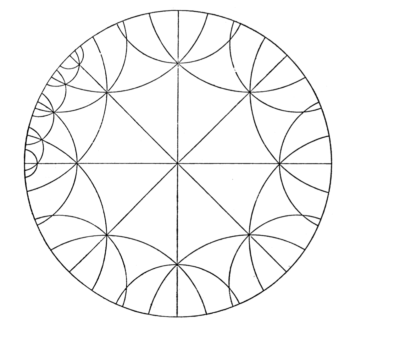
There are now extensive resources on the web for exploring hyperbolic tesselations. This had several major later developments. On the one hand, Poincaré extended this analysis to conformal maps given by second-order linear differential equations with $n$ regular singular points. The conformal image is an $n$-gon bounded by circular arcs. By studying the transformations of these under analytic continuation, Poincaré made the link with non-Euclidean geometry and initiated the modern theories of hyperbolic geometry and automorphic forms. For hypergeometric differential equations of several variables, including those studied by Picard, and Appell and Lauricella, see the works of Deligne and Mostow, [21].

Riemann introduced the idea of monodromy into the study of analytic differential equations. Given a representation of the fundamental group

there is a unique second order rational differential equation with regular singular points $z=0,1,\infty$ with the property that if $f_{1}(z),f_{2}(z)$ is a basis of holomorphic solutions at $x$ then analytic continuation around a loop $\gamma\in\pi_{1}(\mathbb{P}^{1}(\mathbb{C})-\{0,1,\infty\},x)$ yields the linear transformation

Since

to give the monodromy representation is equivalent to giving two-by-two matrices $T_{0},T_{1},T_{\infty}$ such that $T_{0}T_{1}T_{\infty}=1$. These are well-defined up to simultaneous conjugation by an element of $\mathrm{GL}_{2}(\mathbf{C})$. As Katz observes, Riemann proved a stronger result. Namely, it suffices to give the Jordan canonical forms of $T_{0},T_{1},T_{\infty}$ to reconstruct the hypergeometric differential equation. Actually Riemann only considered the case when these were semisimple, so equivalent to diagonal matrices, with eigenvalues $\exp(2\pi i\alpha)$ and $\exp(2\pi i\alpha^{\prime})$; he called the $\alpha,\alpha^{\prime}$ the exponents at the singular point. They are well-defined up to permutation and adding $\mathbf{Z}$. This stronger property, that a differential equation is determined by the Jordan forms of the monodromies at the singular points, is what Katz ([53]) calls rigidity. Rigidity plays an important role in our work.

If $X$ is a connected nonsingular algebraic variety over $\mathbf{C}$ and

is a representation, we get a local system V on the analytic space $X^{an}$. By the Riemann-Hilbert correspondence, this is the solution sheaf to a differential equation, unique up to isomorphism,

with regular singular points at infinity ([16], [51]). If $X$ is a nonsingular algebraic variety over $\mathbf{C}$ we let $X^{an}=X(\mathbf{C})$ be the set of complex points with the classical topology. Assume that $X$ is quasi-projective and connected. Recall the following dictionary: The following categories are equivalent:

• 1.

  Local systems of finite-dimensional $\mathbf{C}$-vector spaces V on $X^{an}$.

• 2.

  Representations $\rho:\pi_{1}(X^{an},x)\to\mathrm{GL}(V)$ on finite-dimensional $\mathbf{C}$-vector spaces $V$.

• 3.

  Holomorphic integrable connections

  $$\nabla:\mathcal{V}^{an}\to\Omega^{1}_{X^{an}/\mathbf{C}}\otimes_{\mathcal{O}_{X^{an}}}\mathcal{V}^{an}$$

  where $\mathcal{V}^{an}$ is a locally free $\mathcal{O}_{X}^{an}$-module of finite rank.

• 4.

  Integrable algebraic connections

  $$\nabla:\mathcal{V}\to\Omega^{1}_{X/\mathbf{C}}\otimes_{\mathcal{O}_{X}}\mathcal{V}$$

  where $\mathcal{V}$ is a locally free $\mathcal{O}_{X}$-module of finite rank, and which have regular singular points “at infinity”.

A reference: [18], [20]. Fix a prime number $\ell$. In this section: scheme = a separated noetherian scheme on which $\ell$ is invertible. We are interested in constructible $\bar{\mathbf{Q}}_{\ell}$-sheaves on $X$, in particular, those that are lisse. In this section: the étale topology is understood. An $\ell$-adic representation of a profinite group $\pi$ on a $\bar{\mathbf{Q}}_{\ell}$-vector space $V$ is a homomorphism

such that there is a finite subextension $E/\mathbf{Q}_{\ell}$ and an $E$-structure $V_{E}$ on $V$ such that $\sigma$ factorizes in a continuous homomorphism $\pi\to\mathrm{GL}(V_{E})$. Recall that a geometric point $\bar{x}$ of a scheme $X$ is a morphism of the spectrum of an algebraically closed field denoted $k(\bar{x})$ to $X$. It is localized in $x\in X$ if its image is $x$. If $X$ is connected and pointed by a geometric point $\bar{x}$, the functor

is an equivalence between the categories of

• 1.

  lisse $\bar{\mathbf{Q}}_{\ell}$-sheaves on $X$;

• 2.

  $\ell$-adic continuous representations of $\pi_{1}(X,\bar{x})$.

Here $\pi_{1}(X,\bar{x})$ is Grothendieck’s fundamental group. Especially if $X=\mathrm{Spec}(k)$ is a field, the category of lisse $\bar{\mathbf{Q}}_{\ell}$-sheaves on $X$ is equivalent to the category of $\ell$-adic representations of $\mathrm{Gal}(\bar{k}/k)$.

If one is working in the category of schemes $X$ of finite type over a perfect field $k$ with algebraic closure $\bar{k}$, and $x\in X(k)$ is a $k$-rational point, by convention we let $\bar{x}$ be the geometric point of $X$ which is the composite $\mathrm{Spec}(\bar{k})\to\mathrm{Spec}(k)\to X$.

More generally, let $S$ be an irreducible scheme of finite type over a field $k$. Then a lisse sheaf $\mathcal{V}$ on $S$ is equivalent to a representation

where $\bar{\eta}$ is a geometric generic point. That is, $\bar{\eta}=\mathrm{Spec}(\overline{k(S)})$ where $\eta$ is the generic point of $S$, and $k(S)=\mathcal{O}_{S,\eta}$ is the function field of $S$.

Recall that there is a canonical exact sequence

Moreover if $k$ has characteristic $0$ and we choose an embedding $k\hookrightarrow\mathbf{C}$, $\pi_{1}(S_{\bar{k}},\bar{\eta})$ is isomorphic to the profinite completion of the Poincaré fundamental group, $\pi_{1}(S^{an},x)$ so this includes the geometric monodromy of $\mathcal{F}$.

Now let $k=\mathbf{F}_{q}$ be a be a finite field of characteristic $p>0$. If $X_{0}$ is a scheme of finite type, we define $X=X_{0}\otimes_{\mathbf{F}_{q}}\bar{\mathbf{F}}_{q}$ and recall that there is a morphism $F:X\to X$ which sends a point with coordinates $x$ to the point with coordinates $x^{q}$. The set of closed points $|X|$ is canonically identified with $X_{0}(\bar{\mathbf{F}}_{q})$, and the Frobenius fixed points $|X|^{F}=X({\mathbf{F}_{q}})$. The set of closed points $|X_{0}|$ is isomorphic to the set of orbits $|X|_{F}$ of $F$; for $x_{0}\in|X_{0}|$ the size of the corresponding orbit $Z$ is $\mathrm{deg}(x_{0})$, which is also the degree of the extension field $k(x)/\mathbf{F}_{q}$. If $\mathcal{F}_{0}$ is a constructible $\bar{\mathbf{Q}}_{\ell}$-sheaf on $X_{0}$ for the étale topology, we let $(X,\mathcal{F})$ be deduced from $(X_{0},\mathcal{F}_{0})$ by extension to the algebraic closure. If $\bar{x}\in|X|$ is a geometric point localized in $x\in|X_{0}|$, we define

The stalk $\mathcal{F}_{\bar{x}}$ is a $\bar{\mathbf{Q}}_{\ell}$-vector space of finite dimension on which $\mathrm{Gal}(k(\bar{x})/k(x))$ acts and therefore

is defined. It is independent of the geometric point $\bar{x}$ localized in $x$, so we can simply denote it by $\det\left(1-t.\mathrm{Frob}_{x}\mid\mathcal{F}_{0}\right)$. The coefficient of $-t$ in this polynomial is the trace $\mathrm{Tr}(\mathrm{Frob}_{x}\mid\mathcal{F}_{0})$. The Grothendieck-Lefschetz trace formula reads:

where $d$ is the dimension of $X$ and $H^{i}_{c}$ is cohomology with proper support. We define the $L$-function

The trace formula is equivalent to the factorization

Let $f:X\to S$ be a proper smooth morphism of algebraic varieties. Then we get local systems:

• 1.

  Over $\mathbf{C}$: $R^{i}f_{*}\mathbf{C}=\mathrm{Ker}(\nabla^{an})$ where

  $$\nabla:H^{i}_{dR}(X/S)\to\Omega^{1}_{S/\mathbf{C}}\otimes_{\mathcal{O}_{S}}H^{i}_{dR}(X/S),\quad H^{i}_{dR}(X/S):=\mathbf{R}^{i}f_{*}\Omega^{\bullet}_{X/S}$$

  is the Gauss-Manin connection on the relative deRham cohomology. Then $(R^{i}f_{*}\mathbf{C})_{s}=H^{i}(X_{s}^{an},\mathbf{C})$. This has regular singular points (Griffiths; see [49]).

• 2.

  $\ell$-adic: $R^{i}f_{*}\mathbf{Q}_{\ell}$ is a lisse $\mathbf{Q}_{\ell}$-sheaf on the étale topology of $S$. The stalk in a geometric point $(R^{i}f_{*}\mathbf{Q}_{\ell})_{\bar{s}}=H^{i}_{et}(X_{s}\otimes_{\kappa(s)}\kappa(\bar{s}),\mathbf{Q}_{\ell})$, which has an action of the Galois group $\mathrm{Gal}(\kappa(\bar{s})/\kappa(s))$.

Let $S=\mathrm{Spec}\,\mathbf{Z}[1/2,\lambda,(\lambda(1-\lambda))^{-1}]$. This is the open subset

For each $\lambda$ we let $E_{\lambda}$ be the projective nonsingular model of the affine curve

This is an elliptic curve with origin at infinity $(x,y,z)=(0,1,0)$ in the projective plane. We get a proper smooth morphism $f:E\to S$ defined over $\mathbf{Z}[1/2]$ with these fibers.

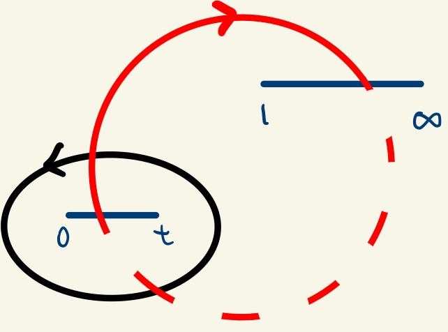
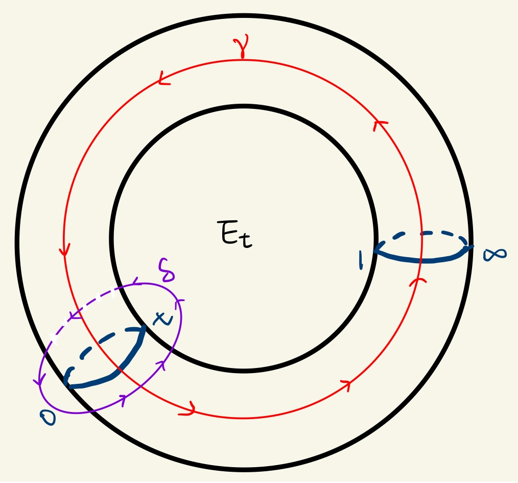
The local system over $\mathbf{C}$ topologically is the flat bundle of $H^{1}(E_{\lambda},\mathbf{C})$ for $\lambda\in\mathbb{P}^{1}(\mathbf{C})-\{0,1,\infty\}$. This latter is the sphere with 3 points removed. We have

isomorphic to a free group on 2 generators. We can represent these by loops starting at the base-point $\lambda_{0}$ and circling once around $0,1,\infty$, respectively. The monodromy can be represented topologically by following the generators of $H^{1}(E_{\lambda},\mathbf{Z})\sim\mathbf{Z}^{2}$ as $\lambda$ moves along these loops. This can be viewed by analytically continuing the period matrix of $E_{\lambda}$ relative to a basis of differential forms. The deRham cohomology $H^{1}_{dR}(E/S)$ is a free $\mathcal{O}_{S}$-module of rank 2. We can take as basis

which is a basis of meromorphic 1-forms of the first and second kind modulo exact forms.

We have the following equation in $H^{1}_{dR}(E/S)$:

Note that $H^{1}_{dR}(E^{an}/S^{an})^{\nabla=0}=R^{1}f_{*}\mathbf{Z}\otimes\mathbf{C}$, where $R^{1}f_{*}\mathbf{Z}$ is a local system of free $\mathbf{Z}$-modules of rank 2 on $S^{an}=\mathbb{P}^{1}(\mathbf{C})-\{0,1,\infty\}$ with a nondegenerate symplectic pairing on it. The dual local system $R_{1}f_{*}\mathbf{Z}$ is the homology local system: $H_{1}(E^{\mathrm{an}}_{\lambda},\mathbf{Z})$. For any local horizontal section $\gamma$ of the dual $R_{1}f_{*}\mathbf{Z}$ of $R^{1}f_{*}\mathbf{Z}$, it follows easily from this that the period $f(\lambda)=\int_{\gamma}dx/y$ is a solution to the differential equation

which is the differential equation satisfied by $\,{}_{2}F_{1}\left[\begin{matrix}1/2&1/2\vskip 3.0pt plus 1.0pt minus 1.0pt\\ &1\end{matrix}\;;\;\lambda\right]$. In fact,

We view a small loop around the interval $[1,\infty]$ as topological cycle $\gamma$ on the Riemann surface $E_{\lambda}$ which is a branched cover of $\mathbb{P}^{1}(\mathbf{C})$ of degree 2.

The monodromy group of this differential equation is projectively equivalent to the principal congruence subgroup $\Gamma(2)\subset\mathrm{SL}_{2}(\mathbf{Z})$. In a suitable basis (we can take so-called vanishing cycles at $1$ and $0$) $\gamma,\delta$ of $H^{1}(E_{t},\mathbf{Z})$ the monodromy matrices are

These generate a subgroup $\Gamma$ of index 2 inside $\Gamma(2)$ acting on the upper half plane with quotient

This map is induced by $\lambda:\mathfrak{H}\to\mathbf{C}\cup\{\infty\}$ where $\lambda(\tau)$ is a generator of the field of modular functions for $\Gamma(2)$. The inverse of this is the multivalued function on $\mathbb{P}^{1}(\mathbf{C})-\{0,1,\infty\}$ given by the period ratio $\tau(\lambda)=\int_{\alpha}\omega_{1}/\int_{\beta}\omega_{1}$ of two independent solutions to this differential equation. The above quotient space, denoted $M_{2}$, is the coarse moduli space of elliptic curves with a level 2 structure.

The $\ell$-adic local system $R^{1}f_{*}\mathbf{Q}_{\ell}$ gives zeta functions of the elliptic curves in the family. For instance, let $\lambda\in\mathbf{F}_{p}$ for an odd prime $p$, $\lambda\neq 0,1$. Then this gives a geometric point $\bar{\lambda}$ of the scheme $S$, and we can identify the fiber

which is the dual of the Tate module of the curve $E_{\lambda}$. Then

For any ring $R$, we denote by $\lambda$ the coordinate on $\mathbb{A}^{1}_{R}$ and by $S$ the open set where $\lambda(1-\lambda)$ is invertible. Given any elements $a,b,c\in R$ we denote by $E(a,b,c)$ the free $\mathcal{O}_{S}$-module of rank 2 with basis $e_{0}$, $e_{1}$, and integrable $R$-connection

Horizontal sections of the dual of $E(a,b,c)$ over an open set $U\subset S$ can be identified with $f\in\Gamma(U,\mathcal{O}_{U})$ which satisfy the differential equation

These hypergeometric equations are two-dimensional factors of the the cohomology of the family of curves $y^{N}=x^{a}(x-1)^{b}(x-\lambda)^{c}$. In effect, the Euler integral representation

shows that the solutions to the differential equation are given by periods of those curves. Given integers $N,a,b,c$ greater that zero, let $Y(N;a,b,c)_{\lambda}$ be the nonsingular projective model of the affine curve in $(x,y)$-space defined by the equation $y^{N}=x^{a}(x-1)^{b}(x-\lambda)^{c}$. We consider this as a family of curves

We have the Gauss-Manin connection

The following theorem gives the structure of this, at least in the generic fiber $\mathrm{Spec}(\mathbf{C}(\lambda))\hookrightarrow U$. Choose an embedding $R\to\mathbf{C}$. Let

This is the open affine subset where $y$ is invertible. It is affine and smooth of relative dimension one over $\mathbf{C}(\lambda)$. The map $(x,y)\to x$ is a finite étale covering

For any root of unity $\xi\in\mu_{n}$ there is an automorphism of $X(N;a,b,c)$ given by $(x,y)\mapsto(x,\xi y)$. This gives the Galois group of the covering $\pi$. Note that the $dx/y^{m}$ defines an element in the character eigenspace $H^{1}_{DR}(X(N;a,b,c)/\mathbf{C}(\lambda))^{\chi(-m)}$ where $\chi(t)(\xi)=\xi^{t}$.

References

- [1] Scott Ahlgren. Gaussian hypergeometric series and combinatorial congruences. In Symbolic computation, number theory, special functions, physics and combinatorics (Gainesville, FL, 1999), volume 4 of Dev. Math., pages 1–12. Kluwer Acad. Publ., Dordrecht, 2001.
- [2] Scott Ahlgren and Ken Ono. A Gaussian hypergeometric series evaluation and Apéry number congruences. J. Reine Angew. Math., 518:187–212, 2000.
- [3] George E. Andrews, Richard Askey, and Ranjan Roy. Special functions, volume 71 of Encyclopedia of Mathematics and its Applications. Cambridge University Press, Cambridge, 1999.
- [4] Donu Arapura. An abelian category of motivic sheaves. Adv. Math., 233:135–195, 2013.
- [5] Donu Arapura. Motivic sheaves revisited. J. Pure Appl. Algebra, 227(8):Paper No. 107125, 22, 2023.
- [6] A. O. L. Atkin, Wen-Ching Winnie Li, Tong Liu, and Ling Long. Galois representations with quaternion multiplication associated to noncongruence modular forms. Trans. Amer. Math. Soc., 365(12):6217–6242, 2013.
- [7] Joseph Ayoub. Les six opérations de Grothendieck et le formalisme des cycles évanescents dans le monde motivique. I. Astérisque, (314):x+466, 2007.
- [8] Joseph Ayoub. Les six opérations de Grothendieck et le formalisme des cycles évanescents dans le monde motivique. II. Astérisque, (315):vi+364, 2007.
- [9] Srinath Baba and Håkan Granath. Genus 2 curves with quaternionic multiplication. Canad. J. Math., 60(4):734–757, 2008.
- [10] Pilar Báyer and Jürgen Neukirch. On automorphic forms and Hodge theory. Math. Ann., 257(2):137–155, 1981.
- [11] Pilar Báyer and Artur Travesa. Uniformizing functions for certain Shimura curves, in the case . Acta Arith., 126(4):315–339, 2007.
- [12] Frits Beukers, Henri Cohen, and Anton Mellit. Finite hypergeometric functions. Pure Appl. Math. Q., 11(4):559–589, 2015.
- [13] Frits Beukers and Gerrit Heckman. Monodromy for the hypergeometric function . Invent. Math., 95(2):325–354, 1989.
- [14] Christina Birkenhake and Herbert Lange. Complex Abelian Varieties, volume 302 of Grundlehren der mathematischen Wissenschaften [Fundamental Principles of Mathematical Sciences]. Springer-Verlag, Berlin, second edition, 2004.
- [15] Alyson Deines, Jenny G. Fuselier, Ling Long, Holly Swisher, and Fang-Ting Tu. Generalized Legendre curves and quaternionic multiplication. J. Number Theory, 161:175–203, 2016.
- [16] Pierre Deligne. Équations différentielles à points singuliers réguliers. Lecture Notes in Mathematics, Vol. 163. Springer-Verlag, Berlin-New York, 1970.
- [17] Pierre Deligne. Formes modulaires et représentations -adiques. In Séminaire Bourbaki. Vol. 1968/69: Exposés 347–363, volume 175 of Lecture Notes in Math., pages Exp. No. 355, 139–172. Springer, Berlin, 1971.
- [18] Pierre Deligne. La conjecture de Weil. I. Inst. Hautes Études Sci. Publ. Math., (43):273–307, 1974.
- [19] Pierre Deligne. Variétés de Shimura: interprétation modulaire, et techniques de construction de modèles canoniques. In Automorphic forms, representations and -functions (Proc. Sympos. Pure Math., Oregon State Univ., Corvallis, Ore., 1977), Part 2, Proc. Sympos. Pure Math., XXXIII, pages 247–289. 1979.
- [20] Pierre Deligne. La conjecture de Weil. II. Inst. Hautes Études Sci. Publ. Math., (52):137–252, 1980.
- [21] Pierre Deligne and George D. Mostow. Monodromy of hypergeometric functions and nonlattice integral monodromy. Inst. Hautes Études Sci. Publ. Math., (63):5–89, 1986.
- [22] Pierre Deligne and Michael Rapoport. Les schémas de modules de courbes elliptiques. In Modular functions of one variable, II (Proc. Internat. Summer School, Univ. Antwerp, Antwerp, 1972), Lecture Notes in Math., Vol. 349, pages 143–316. Springer, Berlin, 1973.
- [23] NIST Digital Library of Mathematical Functions. http://dlmf.nist.gov/, Release 1.1.0 of 2020-12-15. F. W. J. Olver, A. B. Olde Daalhuis, D. W. Lozier, B. I. Schneider, R. F. Boisvert, C. W. Clark, B. R. Miller, B. V. Saunders, H. S. Cohl, and M. A. McClain, eds.
- [24] Bernard Dwork and François Loeser. Hypergeometric series. Japan. J. Math. (N.S.), 19(1):81–129, 1993.
- [25] Bernard Dwork and François Loeser. Hypergeometric series and functions as periods of exponential modules. In Barsotti Symposium in Algebraic Geometry (Abano Terme, 1991), volume 15 of Perspect. Math., pages 153–174. Academic Press, San Diego, CA, 1994.
- [26] Martin Eichler. Quaternäre quadratische Formen und die Riemannsche Vermutung für die Kongruenzzetafunktion. Arch. Math., 5:355–366, 1954.
- [27] Martin Eichler. Eine Verallgemeinerung der Abelschen Integrale. Math. Z., 67:267–298, 1957.
- [28] Noam D. Elkies. Shimura curve computations. In Algorithmic number theory (Portland, OR, 1998), volume 1423 of Lecture Notes in Comput. Sci., pages 1–47. Springer, Berlin, 1998.
- [29] Noam D. Elkies. The Klein quartic in number theory. In The eightfold way, volume 35 of Math. Sci. Res. Inst. Publ., pages 51–101. Cambridge Univ. Press, Cambridge, 1999.
- [30] Ron Evans and John Greene. Clausen’s theorem and hypergeometric functions over finite fields. Finite Fields Appl., 15(1):97–109, 2009.
- [31] Sharon Frechette, Ken Ono, and Matthew Papanikolas. Gaussian hypergeometric functions and traces of Hecke operators. Int. Math. Res. Not., (60):3233–3262, 2004.
- [32] Sharon Frechette, Holly Swisher, and Fang-Ting Tu. A cubic transformation formula for Appell–Lauricella hypergeometric functions over finite fields. Res. Number Theory, 4(2):4:27, 2018.
- [33] Javier Fresán, Claude Sabbah, and Jeng-Daw Yu. Hodge theory of Kloosterman connections. Duke Math. J., 171(8):1649–1747, 2022.
- [34] Lei Fu. -adic GKZ hypergeometric sheaves and exponential sums. Adv. Math., 298:51–88, 2016.
- [35] Lei Fu, Wan Daqing, and Hao Zhang. The -adic Gelfand-Kapranov-Zelevinsky complex. arXiv:1804.05297, to appear, Mathematische Annalen.
- [36] Jenny Fuselier, Ling Long, Ravi Ramakrishna, Holly Swisher, and Fang-Ting Tu. Hypergeometric functions over finite fields. Mem. Amer. Math. Soc., 280(1382), 2022.
- [37] Jenny G. Fuselier. Hypergeometric functions over and relations to elliptic curves and modular forms. Proc. Amer. Math. Soc., 138(1):109–123, 2010.
- [38] Ofer Gabber and François Loeser. Faisceaux pervers -adiques sur un tore. Duke Math. J., 83(3):501–606, 1996.
- [39] Izrail M. Gelfand, Mikhail M. Kapranov, and Andrey V. Zelevinsky. Generalized Euler integrals and -hypergeometric functions. Adv. Math., 84(2):255–271, 1990.
- [40] Matthew Greenberg and John Voight. Computing systems of Hecke eigenvalues associated to Hilbert modular forms. Math. Comp., 80(274):1071–1092, 2011.
- [41] John Greene. Hypergeometric functions over finite fields. Trans. Amer. Math. Soc., 301(1):77–101, 1987.
- [42] Ki-ichiro Hashimoto. Explicit form of quaternion modular embeddings. Osaka J. Math., 32(3):533–546, 1995.
- [43] Jerome W. Hoffman, Wen-Ching Winnie Li, Ling Long, and Fang-Ting Tu. Traces of Hecke Operators via Hypergeometric Character Sums, 2024; arXiv: 2408.02918.
- [44] Rolf-Peter Holzapfel. Geometry and arithmetic around Euler partial differential equations, volume 11 of Mathematics and its Applications (East European Series). D. Reidel Publishing Co., Dordrecht, 1986.
- [45] Jun-ichi Igusa. Arithmetic variety of moduli for genus two. Ann. of Math. (2), 72:612–649, 1960.
- [46] Yasutaka Ihara. Hecke polynomials as congruence functions in elliptic modular case. Ann. of Math. (2), 85:267–295, 1967.
- [47] Hervé Jacquet and Robert P. Langlands. Automorphic forms on . Lecture Notes in Mathematics, Vol. 114. Springer-Verlag, Berlin-New York, 1970.
- [48] Bruce W. Jordan. On the Diophantine arithmetic of Shimura curves, thesis, Harvard University, 1981.
- [49] Nicholas M. Katz. The regularity theorem in algebraic geometry. In Actes du Congrès International des Mathématiciens (Nice, 1970), Tome 1, pages 437–443. 1971.
- [50] Nicholas M. Katz. Algebraic solutions of differential equations (-curvature and the Hodge filtration). Invent. Math., 18:1–118, 1972.
- [51] Nicholas M. Katz. An overview of Deligne’s work on Hilbert’s twenty-first problem. In Mathematical developments arising from Hilbert problems (Proc. Sympos. Pure Math., Northern Illinois Univ., De Kalb, Ill., 1974), volume Vol. XXVIII of Proc. Sympos. Pure Math., pages 537–557. Amer. Math. Soc., Providence, RI, 1976.
- [52] Nicholas M. Katz. Exponential Sums and Differential Equations, volume 124 of Annals of Mathematics Studies. Princeton University Press, Princeton, NJ, 1990.
- [53] Nicholas M. Katz. Rigid local systems, volume 139 of Annals of Mathematics Studies. Princeton University Press, Princeton, NJ, 1996.
- [54] Nicholas M. Katz. Another look at the Dwork family. In Algebra, arithmetic, and geometry: in honor of Yu. I. Manin. Vol. II, volume 270 of Progr. Math., pages 89–126. Birkhäuser Boston, Boston, MA, 2009.
- [55] Michael Klug, Michael Musty, Sam Schiavone, and John Voight. Numerical calculation of three-point branched covers of the projective line. LMS J. Comput. Math., 17(1):379–430, 2014.
- [56] Maxim Kontsevich and Don Zagier. Periods. In Mathematics unlimited—2001 and beyond, pages 771–808. Springer, Berlin, 2001.
- [57] Michio Kuga. Kuga varieties, volume 9 of CTM. Classical Topics in Mathematics. Higher Education Press, Beijing, 2018. Fiber varieties over a symmetric space whose fibers are Abelian varieties, Appendices including a letter by André Weil and an essay by I. Satake.
- [58] Michio Kuga and Goro Shimura. On the zeta function of a fibre variety whose fibres are abelian varieties. Ann. of Math. (2), 82:478–539, 1965.
- [59] Robert P. Langlands. Modular forms and -adic representations. In Modular functions of one variable, II (Proc. Internat. Summer School, Univ. Antwerp, Antwerp, 1972), Lecture Notes in Math., Vol. 349, pages 361–500. Springer, Berlin, 1973.
- [60] Robert P. Langlands. On the zeta functions of some simple Shimura varieties. Canadian J. Math., 31(6):1121–1216, 1979.
- [61] Catherine Lennon. Gaussian hypergeometric evaluations of traces of Frobenius for elliptic curves. Proc. Amer. Math. Soc., 139(6):1931–1938, 2011.
- [62] Catherine Lennon. Trace formulas for Hecke operators, Gaussian hypergeometric functions, and the modularity of a threefold. J. Number Theory, 131(12):2320–2351, 2011.
- [63] Wen-Ching W. Li, Ling Long, and Fang-Ting Tu. A Whipple formula revisited. Matematica, 1(2):480–530, 2022.
- [64] Yi-Hsuan Lin and Yifan Yang. Quaternionic loci in Siegel’s modular threefold. Math. Z., 295(1-2):775–819, 2020.
- [65] Qing Liu. Modèles minimaux des courbes de genre deux. J. Reine Angew. Math., 453:137–164, 1994.
- [66] François Loeser and Claude Sabbah. Caractérisation des -modules hypergéométriques irréductibles sur le tore. C. R. Acad. Sci. Paris Sér. I Math., 312(10):735–738, 1991.
- [67] François Loeser and Claude Sabbah. Équations aux différences finies et déterminants d’intégrales de fonctions multiformes. Comment. Math. Helv., 66(3):458–503, 1991.
- [68] François Loeser and Claude Sabbah. Caractérisation des -modules hypergéométriques irréductibles sur le tore. II. C. R. Acad. Sci. Paris Sér. I Math., 315(12):1263–1264, 1992.
- [69] Ju. I. Manin. Parabolic points and zeta functions of modular curves. Izv. Akad. Nauk SSSR Ser. Mat., pages 19–66, 1972.
- [70] Ju. I. Manin. Periods of cusp forms, and -adic Hecke series. Mat. Sb. (N.S.), pages 378–401, 503, 1973.
- [71] James S. Milne. Introduction to Shimura varieties. In Harmonic analysis, the trace formula, and Shimura varieties, volume 4 of Clay Math. Proc., pages 265–378. Amer. Math. Soc., Providence, RI, 2005.
- [72] Masami Ohta. On -adic representations attached to automorphic forms. Japan. J. Math. (N.S.), 8(1):1–47, 1982.
- [73] Masami Ohta. On the zeta function of an abelian scheme over the Shimura curve. Japan. J. Math. (N.S.), 9(1):1–25, 1983.
- [74] Masami Ohta. On the zeta function of an abelian scheme over the Shimura curve. II. In Galois groups and their representations (Nagoya, 1981), volume 2 of Adv. Stud. Pure Math., pages 37–54. North-Holland, Amsterdam, 1983.
- [75] Maria Petkova and Hironori Shiga. A new interpretation of the Shimura curve with discriminant 6 in terms of Picard modular forms. Arch. Math. (Basel), 96(4):335–348, 2011.
- [76] David P. Roberts and Fernando Rodriguez Villegas. Hypergeometric motives. Notices Amer. Math. Soc., 69(6):914–929, 2022.
- [77] Victor Rotger. Modular Shimura varieties and forgetful maps. Trans. Amer. Math. Soc., 356(4):1535–1550, 2004.
- [78] Anthony J. Scholl. The -adic representations attached to a certain noncongruence subgroup. J. Reine Angew. Math., 392:1–15, 1988.
- [79] René Schoof. Counting points on elliptic curves over finite fields. volume 7, pages 219–254. 1995. Les Dix-huitièmes Journées Arithmétiques (Bordeaux, 1993).
- [80] Hermann A. Schwarz. Ueber diejenigen Fälle, in welchen die Gaussische hypergeometrische Reihe eine algebraische Function ihres vierten Elementes darstellt. J. Reine Angew. Math., 75:292–335, 1873.
- [81] Goro Shimura. Correspondances modulaires et les fonctions de courbes algébriques. J. Math. Soc. Japan, 10:1–28, 1958.
- [82] Goro Shimura. Sur les intégrales attachées aux formes automorphes. J. Math. Soc. Japan, 11:291–311, 1959.
- [83] Goro Shimura. On the zeta-functions of the algebraic curves uniformized by certain automorphic functions. J. Math. Soc. Japan, 13:275–331, 1961.
- [84] Goro Shimura. An -adic method in the theory of automorphic forms. Collected Papers, II:237–272, 1968.
- [85] Goro Shimura. Introduction to the arithmetic theory of automorphic functions, volume 11 of Publications of the Mathematical Society of Japan. Princeton University Press, Princeton, NJ, 1994. Reprint of the 1971 original, Kanô Memorial Lectures, 1.
- [86] Tetsuji Shioda. On rational points of the generic elliptic curve with level structure over the field of modular functions of level . J. Math. Soc. Japan, 25:144–157, 1973.
- [87] Lucy Joan Slater. Generalized hypergeometric functions. Cambridge University Press, Cambridge, 1966.
- [88] Peter Stiller. Special values of Dirichlet series, monodromy, and the periods of automorphic forms. Mem. Amer. Math. Soc., 49(299):iv+116, 1984.
- [89] Kisao Takeuchi. Arithmetic triangle groups. J. Math. Soc. Japan, 29(1):91–106, 1977.
- [90] Kisao Takeuchi. Commensurability classes of arithmetic triangle groups. J. Fac. Sci. Univ. Tokyo Sect. IA Math., 24(1):201–212, 1977.
- [91] John Voight. Quaternion algebras, volume 288 of Graduate Texts in Mathematics. Springer, Cham, [2021] ©2021.
- [92] Yifan Yang. Schwarzian differential equations and Hecke eigenforms on Shimura curves. Compos. Math., 149(1):1–31, 2013.
- [93] Don Zagier. The arithmetic and topology of differential equations. In European Congress of Mathematics, pages 717–776. Eur. Math. Soc., Zürich, 2018.