QED effects on phase transition and Ruppeiner geometry of Euler-Heisenberg-AdS black holes
Abstract
Taking the quantum electrodynamics (QED) effect into account, we study the black hole phase transition and Ruppeiner geometry for the Euler-Heisenberg anti-de Sitter black hole in the extended phase space. For negative and small positive QED parameter, we observe a small/large black hole phase transition and reentrant phase transition, respectively. While a large positive value of the QED parameter ruins the phase transition. The phase diagrams for each case are explicitly exhibited. Then we construct the Ruppeiner geometry in the thermodynamic parameter space. Different features of the corresponding scalar curvature are shown for both the small/large black hole phase transition and reentrant phase transition cases. Of particular interest is that an additional region of positive scalar curvature indicating dominated repulsive interaction among black hole microstructure is present for the black hole with a small positive QED parameter. Furthermore, the universal critical phenomena are also observed for the scalar curvature of the Ruppeiner geometry. These results indicate that the QED parameter has a crucial influence on the black hole phase transition and microstructure.
pacs:
04.70.Dy, 05.70.Ce, 04.50.KdI Introduction
Due to the earliest pioneering work of Hawking and Bekenstein on the temperature and entropy of black holes, it has shown that there is a deep connection between gravity, quantum mechanics, and thermodynamics Bekensteing73 ; hawking1975particle ; hawking1976black . Equipped with the established four laws of black hole thermodynamics bardeen1973four , the study of the thermodynamics becomes one of the increasingly active areas in black hole physics. Motivated by the anti-de Sitter/conformal field theory (AdS/CFT) correspondence witten1998anti ; maldacena1998large , the Hawking-Page phase transition hawking1983thermodynamics between the stable large Schwarzschild AdS black hole and thermal space was interpreted as the confinement/deconfinement phase transition of the gauge field witten1998thermal . The phase transition was also extended to the charged and rotating AdS black hole cases chamblin1999charged ; chamblin1999holography ; caldarelli2000thermodynamics .
Recently, it was found in the AdS space that, by interpreting the cosmological constant as thermodynamic pressure kastor2009enthalpy ; dolan2011pressure ; cvetivc2011black , the black hole systems are analog to everyday thermodynamical systems. In this extended thermodynamic phase space, the charged small/large AdS black hole phase transition is similar to the gas-liquid phase transition of Van der Waals (VdW) fluid Kubiznak:2012wp . Subsequently, more interesting black hole phase transitions and phase structures, such as reentrant phase transition NaveenaKumara:2020biu ; altamirano2013reentrant , isolated critical point dolan2014isolated , triple point altamirano2014kerr ; wei2014triple ; frassino2014multiple , and superfluid black hole phase hennigar2017superfluid , have been uncovered.
Understanding black hole microstructure has to be a huge challenge. Although the string theory Strominger:1996sh ; Maldacena:1996gb ; Callan:1996dv ; Horowitz:1996fn , fuzzy ball model Lunin:2001jy ; Lunin:2002qf , and pierced horizons Rovelli:1996dv have made great progress, more questions remain to be solved. As proposed in Refs. Wei:2015iwa ; Wei:2019uqg , the study of black hole phase transition can also be applied to this challenge with the assumption that the micro-degree of freedom is measured by the underlying molecules of the black hole. Combining with the Ruppeiner geometry ruppeiner1995riemannian , the characteristic black hole microstructure was tested. Its scalar curvature of the corresponding geometry is an important tool for exploring the microstructure of a black hole. Via the empirical observation that the positive or negative scalar curvature corresponds to the repulsive or attractive interaction among these underlying black hole molecules. Such empirical result was supported by many studies of different fluid systems, such as ideal fluids ingarden1978information , Van der Waals (VdW) fluids janyszek1990riemannian , one-dimensional Ising models, quantum gases ruppeiner1981application ; janyszek1989magnetic . More significantly, when considering the microscopic model and the equation of state, a possible interpretation of the empirical observation was given and the corresponding molecular potential is constructed in Ref. Wei:2021hva .
In view of the ”hard-core” model, there is only the dominated attractive interaction for the VdW fluid. However for the charged AdS black holes, the dominated repulsive interaction emerges for the small black hole with high temperature Wei:2019yvs , which uncovers an interesting phenomenon for the black hole microstructure. After generalizing the study to the modified gravity Wei:2019ctz , it was found that the dominated repulsive interaction may not emerge, while the attractive interaction is universal.
On the other hand, black hole solutions with nonlinear electrodynamics gain great interest. In particular, this theory can be viewed as a low-energy limit from string theory or D-brane physics, where Abelian and non-Abelian nonlinear electrodynamic Lagrangians could be produced. The thermodynamics of the charged Born-Infeld (BI) AdS black holes was considered in Ref. Gunasekaran:2012dq . The present of the BI vacuum polarization governs a rich black hole phase transition. The study was also extended to higher dimensions, and the small/large black hole phase transition was found to be universal Zou:2013owa . Another widely concerned nonperturbative one-loop effective Lagrangian of nonlinear electromagnetic fields originates from Heisenberg and Euler heisenberg1936folgerungen . Within the QED framework, it was reformulated by Schwinger schwinger1951gauge . The black hole solutions corresponding to the effective Lagrangian have been worked out ruffini2013einstein . In Refs. Magos:2020ykt ; Li:2021ygi , the first law of black hole thermodynamics and Smarr formula were found to be consistent with each other when the vacuum polarization parameter is included in. The phase transition was preliminarily studied. At the critical point, the standard mean field theory exponents were obtained.
Motivated by it, we in this paper will thoroughly study the phase transition for the charged Euler-Heisenberg (EH)-AdS black holes by taking the QED effect into account. The small/large black hole phase transition and reentrant phase transition are found to exist in different regions of the parameter space. The phase diagrams and phase structures are completely exhibited. Then based on its phase diagram, we constructed the Ruppeiner geometry for the charged EH-AdS black hole. The feature of the scalar curvature is also obtained. Further employing with the empirical observation of the Ruppeiner geometry, we disclose the particular interesting property of the microstructure for the black holes.
This article is organized as follows. In Sec. II, we firstly review the thermodynamics for the charged EH-AdS black hole. Then in different regions of the parameter space, we study the small/large black hole phase transition and reentrant phase transition, respectively. The phase diagrams are clearly exhibited. In Sec. III, the Ruppeiner geometry is constructed. Employing with the corresponding scalar curvature, we explore the characteristic black hole microstructure under the small/large black hole phase transition and reentrant phase transition. Novel properties are found. Finally, the conclusions and discussions are given in Sec. IV.
II Thermodynamics and phase transition of Euler-Heisenberg-AdS black hole
In this section, we would like to briefly review the thermodynamics for the charged EH-AdS black hole with the QED correction ruffini2013einstein , and then study its phase transition in a complete parameter space, where the small/large black hole phase transition, reentrant phase transition will be clearly exhibited.
II.1 Thermodynamics and critical points
The action of the EH theory with cosmological constant in four-dimensional spacetime is salazar1987duality
| (1) |
| (2) |
Here , , and are the determinant of the metric tensor, cosmological constant, and Ricci curvature tensor, respectively. The term is the Lagrangian of the nonlinear electrodynamics which depends on the electromagnetic invariants and . The Maxwell field strength , and is the corresponding vector potential. The parameter appearing in formula (2) can be used to measure the strength of the QED correction, which is related to the mass and charge of the electron, and thus we call it the QED parameter. When =0, the influence of the QED term will vanish.
For a static spherically symmetric charged EH-AdS black hole solution, the line element is Magos:2020ykt
| (3) |
where the metric function is given by
| (4) |
where and are the mass and electric charge of the black hole, respectively. When , this solution reduces to the Reissner-Nordström (RN) AdS black hole solution.
The radius of the outer black hole event horizon is the largest root of , which can be obtained by solving
| (5) |
In term of , the mass can be expressed as
| (6) |
Using the “Euclidean trick”, the Hawking temperature is
| (7) |
In the extended phase space, the cosmological constants was interpreted as the pressure via kastor2009enthalpy . Accordingly, the black hole mass will act as the enthalpy of the thermodynamic system rather than the internal energy. Then the first law has the following form
| (8) |
where is the conjugate quantity to the QED parameter . The entropy , thermodynamic volume , electric potential , and can be calculated as
| (9) | ||||
| (10) | ||||
| (11) | ||||
| (12) |
It is straightforward to confirm the following Smarr formula holds
| (13) |
From Eq. (7), the equation of state can be written as
| (14) |
In term of thermodynamic volume , the equation of state reads
| (15) |
We plot the pressure as a function of the specific volume for fixed temperature in Fig. 1 with () and () being two representative examples, respectively. In Fig. 1, we can see that there are two extremal points (marked with red dots) for . And these points divide the isothermal curve into three branches. Two of them are the small black hole and large black hole locating at the left and right sides of the isothermal curve respectively, while the middle branch is for the intermediate black hole. According to the heat capacity, these black hole branches with negative slope are thermodynamic stable, while those with positive slope are unstable. Thus the small and large black holes are stable and the intermediate black hole is unstable. Making the use of the Maxwell equal area law, one can construct two equal areas along each isothermal curve to obtain the phase transition point. On the other hand, with the increase of the temperature, these two extremal points get closer and coincide with each other at . When , there is no extremal point anymore. Quite differently, for a positive QED parameter, i.e., , there are three extremal points in Fig. 1 for . When the temperature approaches its critical value, two of them coincide, while the other one continues to exist even when the temperature is above its critical value. Below the critical temperature, the nonmonotonic behavior of the isothermal curve also allows one to construct two equal areas indicating the existence of the black hole phase transition.


The critical point can be determined by the following conditions
| (16) |
These conditions gives a third degree equation for
| (17) |
When , the equation (17) has three real roots Magos:2020ykt
| (18) |
One notes that gives a negative volume, and it should be excluded. Therefore, only =0 and 1 is allowed, and the critical temperature and pressure are given by
| (19) |
The critical volume is defined as depending on the charge and QED parameter . It is worth noting that when the QED parameter , the equation (17) has no real root, and thus no critical point exists. For , there is a real root (=0) giving one critical point.
In summary, there are two characteristic types of phase transition. The first type is for , which admits one critical point, and the phase transition is the similar to the gas-liquid phase transition of VdW fluid. For the other type with QED parameter , two critical points can be found, and we shall see there exists the reentrant phase transition.
In the extended phase space, we can introduce the reduced quantities , , ,
| (20) |
Then the equation of state (15) takes the following form
| (21) |
where . In the canonical ensemble, the Gibbs free energy , which reads
| (22) |
In general, the first-order phase transition can be determined by the swallow tail behavior of the Gibbs free energy. In the following sections, we shall study the phase transition via the behavior of the Gibbs free energy.
II.2 Van der Waals type phase transition with
For this case, we take and for example. The Gibbs free energy is plotted as the temperature in Fig. 2 for different values of the pressure. When , we observe the characteristic swallow tail behavior indicating the coexistence of the black hole phase transition. As the pressure increases, the shape of the swallowtail becomes smaller, and it shrinks to a point when . Further increasing the temperature, the behavior completely disappears. Then the Gibbs free energy turns to a smooth function of the temperature.


In order to clearly show the phase transition, we describe the Gibbs free energy in Fig. 2 with . After a simple calculation, we find that the small and large black hole branches in blue and red solid curves have positive heat capacity, and thus they are thermodynamic stable. Whereas these branches in dashed curve are unstable or metastable. Considering that a system always prefers a state of low Gibbs free energy, the system will undergo a first-order phase transition from a small black hole (SBH) phase to a large black hole (LBH) phase with the increase of the temperature. The phase transition point exactly locates at the intersection of the swallow tail behavior. Thus it is easy to see that this phase transition is similar to the liquid-gas phase transition of a VdW fluid.
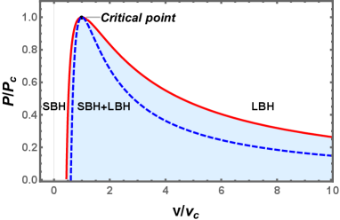
The phase structures of the charged EH-AdS black hole are given in Fig. 3, from which we find that it shares a similar phase diagram with the VdW fluid. In the - diagram, the first-order coexistence curve of the small and large black holes starts at and ends at the critical point, which divides the plane into two regions corresponding to the small and large black hole phases, respectively. Considering that the equation of state is not applicable in the shadow region, we use the spinodal curve marked with the blue dashed curve to distinguish the metastable phase from the coexistence phase of the black hole. The spinodal curve is determined by
| (23) |
Obviously, the spinodal curve meets the coexistence curve at the critical point.
II.3 Reentrant phase transition case with
For this case, two critical points can be found. The corresponding phase transition is the reentrant phase transition including a zeroth-order and a first-order phase transitions at a certain region of the temperature or pressure. Here we shall study the reentrant phase transition for the charged EH-AdS black hole.
As expected, the first-order phase transition can be determined by constructing two equal areas according to the Maxwell’s equal area law. As we shown in Fig. 1, the isotherm curves exhibit a nonmonotonic behavior in - plane. So we can construct two equal areas between two stable black hole branches. However, as pointed out in Ref. wei2015clapeyron , the equal areas should be constructed in - plane rather than - plane. Alternatively, the Maxwell’s equal area law also holds in the - plane for giving pressure both in ordinary or reduced parameter space
| (24) |
where denotes the reduced temperature of phase transition and and are the reduced entropy of the corresponding coexistence small and large black holes. Taking =0.4 as an example, the Maxwell’s equal area law is fulfilled in the - plane in Fig. 4. The black curves denote the small black hole and large black hole branches, respectively. The red curves are for the two metastable branches, the superheated small black hole branch and the supercooled large black hole branch. The blue curve with a negative slope is an unstable branch, and it is substituted by a horizontal line according to the equal area law. The area under the isobaric curve from to is required to equal the area enclosed by the rectangle under the isothermal horizontal line, so the areas of the two shadow regions are equal. These two black dots are the spinodal points, which separate the metastable branches from the unstable branch. Then the pressure and temperature corresponding to the isothermal horizontal line are just that of the phase transition point.


We depict the Gibbs free energy for these two types of phase transitions in Fig. 5. In Fig. 5, the small/large black hole phase transition is analyzed for the reduced pressure . As the temperature increases, the system jumps directly from the SBH phase (red solid line) to the LBH phase (blue solid line), and the volume of the black hole directly undergoes a sudden change when the temperature is equal to the phase transition temperature. For the black hole branches described by the black dashed lines, their heat capacity is negative indicating thermodynamically instability. Note that although these black hole branches described by the dotdashed lines in the Fig. 5 have a positive heat capacity, they do not have the lowest free energy for a fixed temperature, and thus they are metastable black hole branches. In addition to the small/large black hole phase transition, another new zeroth-order phase transition emerges in Fig. 5. When the zeroth-order phase transition occurs, the black hole system jumps from the LBH phase to the SBH phase. Moreover, not only the volume of a black hole will undergo sudden changes, but the Gibbs free energy will also change drastically. In short, the black hole system firstly undergoes a zeroth-order phase transition from LBH phase to SBH phase and then returns to LBH phase through the small/large black hole phase transition with the increase of the temperature. This phase transition of such pattern is called the reentrant (large/small/large BH) phase transition.


The phase diagrams of reentrant phase transition are shown in Fig. 6. Similar to the case of the VdW phase transition type, the coexistence curve (red solid line) divides the parameter space into two regions in Fig. 6. Above and below the coexistence curve are the SBH phase and the LBH phase, respectively. The zeroth-order phase transition line marked with green solid line connects the first-order coexistence curve and the minimum temperature curve. The phase diagram is also exhibited in - plane in Fig. 6. The critical point divides the coexistence curve into left and right parts corresponding to the coexistence small black hole and the large black hole, respectively. The small and large black hole regions locate at the left and right.
In Fig. 7, we plot the difference of the volume among the first-order phase transition as a function of the temperature and pressure, respectively. It is obvious that below the critical point, has a finite value indicating a sudden change during the black hole phase transition. However, when the critical point is reached, vanishes, which means that one could not distinguish the small and large black holes anymore. Considering the behavior of , it can be regarded as an order parameter to characterize the phase transition.


Near the critical point, the critical exponent of can be calculated, see Ref. Magos:2020ykt . However, in the calculation, the specific volume is used in constructing the equal area law, which as we pointed out is inappropriate. Here we would like to make use of the thermodynamic volume instead, and to see whether the result keeps unchanged. Using the relationship between thermodynamic volume and specific volume , we get . Then the formula (21) can be expressed as
| (25) |
where . Let the first term in the previous equation be the function , so (25) can be written as
| (26) |
The Taylor expansion in the vicinity of the critical point at and is written as
| (27) |
From the definition of the critical point, the equation (II.3) must meet the following conditions
| (28) |
Therefore, Eq. (II.3) can be simplified to
| (29) |
Taking and , the previous expression become
| (30) |
where we have defined . From Maxwell’s equal area law we obtained
| (31) |
where and are the volumes of the coexistence small and large black hole respectively. For an isothermal process, the pressure is equal to , i.e. , which reads
| (32) |
Combining (31) and (32), we have
| (33) |
The critical exponent is related to the order parameter , namely with the change of volume at the phase transition for a given isotherm process,
| (34) |
Therefore the critical exponent is
| (35) |
As a result, we can see that the choose of the specific volume or thermodynamic volume does not change the value of the critical exponent . However when applying the Maxwell equal area law, we should choose the thermodynamic volume rather than the specific volume.
III Ruppeiner geometry and microstructure
In this section, we would like to construct the Ruppeiner geometry for the charged EH-AdS black hole. Via the curvature scalar, the microstructure will be tested.
III.1 Ruppeiner geometry
Here, we firstly give a brief introduction for the Ruppeiner geometry and then calculate the curvature scalar for the charged EH-AdS black hole.
Let us consider a thermodynamically isolated system in equilibrium with the total entropy . The system is divided into two subsystems, the small system we consider and its large environment. Their entropies are denoted by and with . We suppose that the total entropy of the system is described by two independent thermodynamic variables and . The total entropy of the system can be written as
For an equilibrium system, the entropy reaches its maximum locally. We perform Taylor expansion in the neighborhood of this local maximum
| (36) |
where a zeroth-order term is the local maximum of entropy at . The entropy of an isolated system in equilibrium is conserved under virtual change. This shows that the first derivative of the entropy vanishes, and thus we get
| (37) |
It is worth noting that is a thermodynamic extensive quantity, and it is the same order of magnitude as the entropy of the entire system. Therefore, its derivative with respect to the intensive quantity is much smaller than the derivative of , which can be ignored. Therefore, the probability of finding the system in the internals (, ) and (, ) will be
| (38) |
where is Boltzmann’s constant. With (37), the line element of Ruppeiner geometry measuring the distance between two neighboring fluctuation states can be written as
| (39) | ||||
| (40) |
Because can measure the distance between two neighboring fluctuation states, the thermodynamic metric potentially contains some information about the microstructure of the system.
When we choose the thermodynamic coordinates to be the temperature and the volume , the Helmholtz free energy is the thermodynamic potential. The corresponding line element can be written as follows Wei:2019uqg
| (41) |
where is the heat capacity at constant volume. Using the convention in the literature ruppeiner1995riemannian , we can directly calculate the corresponding scalar curvature of the line element
| (42) |
It should be noted that the sign of scalar curvature characterizes the type of interaction between two microscopic molecules in a given system ruppeiner2010thermodynamic , i.e. and represent dominated repulsive interaction and attractive interaction, respectively. For VdW fluid, the study shows that it has a negative scalar curvature indicating the dominated attractive interaction among these underlying molecules. In addition, when , the interaction of repulsion and attraction reaches equilibrium dolan2015intrinsic .
For the charged EH-AdS black hole, the heat capacity at constant volume vanishes. We adopt the treatment of Ref. Wei:2019yvs , the new normalized scalar curvature is
| (43) |
Using the equation of state (15), the normalized scalar curvature of the charged EH-AdS black hole reads
| (44) |
where
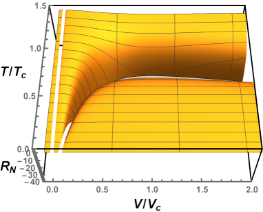
We plotted the scalar curvature as a function of and in Fig. 8 for the small/large black hole phase transition and reentrant phase transition. It can be observed that the surface of the normalized scalar curvature is concave where the scalar curvature diverges. Besides, compared with the VdW type phase transition, a new divergence occurs in the reentrant phase transition when the reduced volume is close to zero.

III.2 Van der Waals type phase transition with
As we shown above, there is the small/large black hole phase transition of VdW-like for the case.
In order to show the details, we take and , and illustrate the normalized scalar curvature as a function of for fixed reduce temperature = 0.4, 0.8, 1.0 and 1.2 in Fig. 9. For , there are two divergent points of the normalized scalar curvature . It can be found that these two points will come closer as the temperature increases. When the critical temperature is approached, these two points merge. When , the normalized scalar curvature does not diverge while keeps finite values. In most of the parameter space, is negative, while in a small region of for = 0.4 shown in the inset of Fig. 9, is positive. This phenomenon indicates that the dominated repulsive interaction may exist in some parameter regions.


From the analysis of the normalized scalar curvature , it is easy to know that the divergent point of satisfies the spinodal point condition , which gives
| (45) |
After a simple calculation, the specific expression of the sign changing curve corresponding to reads
| (46) |
which indicates that the temperature of the sign changing curve is half of the temperature of the spinodal curve Wei:2019uqg ; Wei:2019yvs .
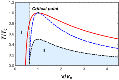
In Fig. 10, the sign changing curve (black dotdashed), spinodal curve (blue dashed), and the coexistence curve (red solid) are displayed. The shadow regions I and II have positive scalar curvature, while the other regions are for negative scalar curvature. Considering that the equation of state for the charged EH-AdS black hole in region II is no longer valid, this region needs to be excluded. However, in region I, the small black hole with high temperature still admits the dominated repulsive interaction. This is similar to the situation of the charged RN-AdS black holes, while different from the neutral black hole in Gauss-Bonnet gravity Wei:2019ctz ; Zhou:2020vzf .
We show the behavior of along the coexistence small and large black holes in Fig. 10. It is easy to see that both them go to negative infinity at the critical temperature indicating the existence of the critical exponent. Moreover, we can also find that of the coexistence small black hole is always above that of the large black hole. At low temperature, the coexistence small black hole has a positive value, which is consistent with that of Fig. 10.

Since the critical exponent can provide us with some universal properties, we now turn to calculate it for the scalar curvature at the critical point. Here it is natural to assume the normalized scalar curvature near the critical point has the following form johnston2014advances
| (47) |
or equivalently,
| (48) |
Via calculating near the critical point, we obtain the following fitting results
| (49) | |||||
| (50) |


The numerical results (small red dots) and fitting results (blue solid lines) are shown in Fig. 11. It is obvious that the numerical and fitting results are highly consistent with each other. The slopes obtained by fitting the coexistence curves of small and large black holes are respectively =2.0365 and =1.9636. Taking into account the error of the numerical calculation, we can say that the critical exponent is , which is the same as that of the VdW fluid.
Moreover, using the intercept obtained by fitting results, we obtain a dimensionless constant
| (51) |
It is the same value with the charged AdS black holes and VdW fluids, and is also consistent with the result obtained in Ref. Magos:2020ykt via expanding the equation of state near the critical point at the first leading term.
III.3 Reentrant phase transition case with
We explore the underlying microstructure of the black hole that results in reentrant phase transition with =1 and =1 by using the similar method. The behavior of against the reduced thermodynamic volume for a fixed temperature is shown in Fig. 12. Comparing with the VdW phase transition, we observe that the scalar curvature of the reentrant phase transition has an additional divergent point near the origin. The reason is when , there are three extremal points on each isothermal curve, see Fig. 1. As the temperature increases, the evolution behavior of other two divergent points is very similar to the case of the VdW-like phase transition. Furthermore, when the temperature is higher than its critical value, the additional divergent point still exists. On the other hand, when the reduced volume is close to the origin, one observes a positive scalar curvature as expected.


The first-order coexistence curve, zeroth-order phase transition curve, spinodal curve, and sign changing curve are depicted in Fig. 13. In the shadow regions I, II, and III, the scalar curvature takes positive values. Compared with the VdW-like phase transition, the number of the shadow regions is three instead of two. It can be seen that the leftmost of the coexistence curve of small black hole ends at the spinodal curve and it indicates that there is a divergence. On the other hand, one should note that the black hole does not exist in region I.
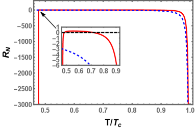
We also plot the normalized scalar curvature along the coexistence small and large black hole curves as a function of temperature in Fig. 13. Along the coexistence curve, negatively diverges at the critical point for both the small and large black holes. However, different from the previous VdW-like phase transition, the scalar curvature of the small black hole gains a new divergence when the reduce temperature is around 0.48. While for the coexistence large black hole, there is no such phenomenon. The reason for this new divergence is that the leftmost of the coexistence small black hole curve is located on the spinodal curve, but the large black hole is not.

Near the critical point, the fitting results for the coexistence small and large black holes are given by
| (52) | |||||
| (53) |


The numerical results and the fitting results are shown in Fig. 14 with highly consistent with each other. The fitting coefficients of the small and large black holes are respectively =1.9536, =2.0426. Taking into account the error of the calculation, we get the critical exponent . The dimensionless constant is
| (54) |
which is the same as that of the VdW-like phase transition.
IV conclusion
In this paper, We have studied the phase transition and Ruppeiner geometry in different ranges of QED parameter in the extended phase space. For and , we observed the small/large black hole phase transition and reentrant phase transition respectively. While for , there will be no the first-order phase transition. In these different ranges, we explored the black hole microstructure and different potential interactions are uncovered for the charged EH-AdS black hole.
In the first part, we investigated the thermodynamic properties of the black hole phase transition. Treating the cosmological constant and QED parameter as two new variables, we got the first law of the black hole thermodynamics and the Smarr formula hold. We also confirmed that they are consistent with each other in the extended phase space. Further, via the Hawking temperature, we obtained the equation of state. Employing it, the critical point is obtained. It is shown that for , , and , one, two, and zero critical points can be observed. According to it, we studied the phase transition in these parameter ranges.
For negative QED parameter , we observed a characteristic swallow tail behavior of the Gibbs free energy below the critical point, which indicates there is the typical first-order black hole phase transition. The phase diagrams are also explicitly shown. When , two critical points observed indicate a rich phase transition beyond the small/large black hole phase transition. For some certain values of the temperature or pressure, four black hole branches are found with two of them being unstable and the other two stable. From the behavior of the Gibbs free energy, these two stable branches form a reentrant phase transition. We then exhibited its phase diagrams, which is quite different from the small/large black hole phase transition of the VdW type. When the QED parameter has a large value such that , only one black hole branch is stable, and thus no black hole phase transition exists.
The second part is devoted to the study of microstructure by using the Ruppeiner geometry. Taking (, ) as two fluctuation coordinates in thermodynamic phase space, we constructed the Ruppeiner geometry and calculated the corresponding normalized scalar curvature for the charged EH-AdS black holes. The scalar curvature behaves quite differently for the small/large black hole phase transition and reentrant phase transition, which may be due to the fact that they have different phase structures. For the small/large black hole phase transition, the normalized scalar curvature has two divergent points for each isothermal curve at most. While for the reentrant phase transition, an additional divergent point near small volume is observed.
Via the empirical observation of the Ruppeiner geometry, we found that for the black hole with negative QED parameter, the repulsive interaction among its microstructure will dominate for the small black hole with high temperature, while the attractive interaction dominates for other black holes. This result is similar to that of the charged AdS black hole without the QED parameter. For the charged EH-AdS black hole with small QED parameter, another region of positive scalar curvature emerges. It is below while not surrounded by the coexistence curve of the first-order phase transition. So for this case, different from the small/large black hole phase transition, the equation of state is applicable. Therefore, the low temperature black hole could have dominated repulsive interaction.
Furthermore, the behavior of the scalar curvature along the first-order coexistence curve of small and large black holes is carefully analyzed. For the case =-1.5 and =1, the scalar curvature for both the coexistence small and large black holes decreases and goes to negative infinity at the critical temperature. However for =1 and =1, a reentrant phase transition is present. Except for the divergent point near the critical point, the scalar curvature of the coexistence small black hole also diverges near =0.48, which is mainly because that the starting point of the coexistence small black hole is on the spinodal curve. This is also one of the novel features for the reentrant phase transition.
In particular, through the numerical calculation, we observed a critical exponent 2 and a dimensionless constant near the critical point for the scalar curvature. This result is the same as that of other black holes and VdW fluid suggesting a result of the mean field theory.
Our work gives a complete study of the phase transition and microstructure for the charged EH-AdS black hole. The effects of the QED parameter on the black hole thermodynamics are examined in detail. Via the geometric method, the interaction among the microstructures is uncovered. These results help us peek into the nature of the black hole with a QED correction from the viewpoint of thermodynamics.
Acknowledgements
This work was supported by the National Natural Science Foundation of China (Grants No. 12075103, No. 11675064, and No. 12047501).
References
- (1) J. D. Bekenstein, Black holes and entropy, Phys. Rev. D 7, 2333 (1973).
- (2) S. W. Hawking, Particle creation by black holes, Commun. Math. Phys. 43, 199 (1975), [Erratum: Commun. Math. Phys. 46, 206 (1976)].
- (3) S. W. Hawking, Black holes and thermodynamics, Phys. Rev. D 13, 191 (1976).
- (4) J. M. Bardeen, B. Carter, and S. W. Hawking, The Four laws of black hole mechanics, Commun. Math. Phys. 31, 161 (1973).
- (5) E. Witten, Anti-de Sitter space and holography, Adv. Theor. Math. Phys. 2, 253 (1998), [arXiv:hep-th/9802150].
- (6) J. M. Maldacena, The large N limit of superconformal field theories and supergravity, Adv. Theor. Math. Phys. 2, 231 (1998), [arXiv:hep-th/9711200].
- (7) S. W. Hawking and D. N. Page, Thermodynamics of black holes in anti-de Sitter space, Commun. Math. Phys. 87, 577 (1983).
- (8) E. Witten, Anti-de Sitter space, thermal phase transition, and confinement in gauge theories, Adv. Theor. Math. Phys. 2, 505 (1998), [arXiv:hep-th/9803131].
- (9) A. Chamblin, R. Emparan, C. V. Johnson, and R. C. Myers, Charged AdS black holes and catastrophic holography, Phys. Rev. D 60, 064018 (1999), [arXiv:hep-th/9902170].
- (10) A. Chamblin, R. Emparan, C. V. Johnson, and R. C. Myers, Holography, thermodynamics and fluctuations of charged AdS black holes, Phys. Rev. D 60, 104026 (1999), [arXiv:hep-th/9904197].
- (11) M. M. Caldarelli, G. Cognola, and D. Klemm, Thermodynamics of Kerr-Newman-AdS black holes and conformal field theories, Class. Quant. Grav. 17, 399 (2000), [arXiv:hep-th/9908022].
- (12) D. Kastor, S. Ray, and J. Traschen, Enthalpy and the mechanics of AdS black holes, Class. Quant. Grav. 26, 195011 (2009), [arXiv:0904.2765 [hep-th]].
- (13) B. P. Dolan, Pressure and volume in the first law of black hole thermodynamics, Class. Quant. Grav. 28, 235017 (2011), [arXiv:1106.6260 [gr-qc]].
- (14) M. Cvetic, G. W. Gibbons, D. Kubiznak, and C. N. Pope, Black hole enthalpy and an entropy inequality for the thermodynamic volume, Phys. Rev. D 84, 024037 (2011), [arXiv:1012.2888 [hep-th]].
- (15) D. Kubiznak and R. B. Mann, - criticality of charged AdS black holes, JHEP 07, 033 (2012), [arXiv:1205.0559 [hep-th]].
- (16) A. Naveena Kumara, C. L. Ahmed Rizwan, K. Hegde, M. S. Ali, and K. M. Ajith, Ruppeiner geometry, reentrant phase transition, and microstructure of Born-Infeld AdS black hole, Phys. Rev. D 103, 044025 (2021), [arXiv:2007.07861 [gr-qc]].
- (17) N. Altamirano, D. Kubiznak, and R. B. Mann, Reentrant phase transitions in rotating anti de Sitter black holes, Phys. Rev. D 88, 101502 (2013), [arXiv:1306.5756 [hep-th]].
- (18) B. P. Dolan, A. Kostouki, D. Kubiznak, and R. B. Mann, Isolated critical point from Lovelock gravity, Class. Quant. Grav. 31, 242001 (2014), [arXiv:1407.4783 [hep-th]].
- (19) N. Altamirano, D. Kubiznak, R. B. Mann, and Z. Sherkatghanad, Kerr-AdS analogue of triple point and solid/liquid/gas phase transition, Class. Quant. Grav. 31, 042001 (2014), [arXiv:1308.2672 [hep-th]].
- (20) S.-W. Wei and Y.-X. Liu, Triple points and phase diagrams in the extended phase space of charged Gauss-Bonnet black holes in AdS space, Phys. Rev. D 90, 044057 (2014), [arXiv:1402.2837 [hep-th]].
- (21) A. M. Frassino, D. Kubiznak, R. B. Mann, and F. Simovic, Multiple reentrant phase transitions and triple points in lovelock thermodynamics, JHEP 09, 080 (2014), [arXiv:1406.7015 [hep-th]].
- (22) R. A. Hennigar, R. B. Mann, and E. Tjoa, Superfluid black holes, Phys. Rev. Lett. 118, 021301 (2017), [arXiv:1609.02564 [hep-th]].
- (23) A. Strominger and C. Vafa, Microscopic origin of the Bekenstein-Hawking entropy, Phys. Lett. B 379, 99 (1996), [arXiv:hep-th/9601029 [hep-th]].
- (24) J. M. Maldacena and A. Strominger, Statistical entropy of four-dimensional extremal black holes, Phys. Rev. Lett. 77, 428 (1996), [arXiv:hep-th/9603060 [hep-th]].
- (25) C. G. Callan and J. M. Maldacena, D-brane approach to black hole quantum mechanics, Nucl. Phys. B 472, 591 (1996), [arXiv:hep-th/9602043 [hep-th]].
- (26) G. T. Horowitz and A. Strominger, Counting states of near extremal black holes, Phys. Rev. Lett. 77, 2368 (1996), [arXiv:hep-th/9602051 [hep-th]].
- (27) O. Lunin and S. D. Mathur, AdS/CFT duality and the black hole information paradox, Nucl. Phys. B 623, 342 (2002), [arXiv:hep-th/0109154 [hep-th]].
- (28) O. Lunin and S. D. Mathur, Statistical interpretation of Bekenstein entropy for systems with a stretched horizon, Phys. Rev. Lett. 88, 211303 (2002), [arXiv:hep-th/0202072 [hep-th]].
- (29) C. Rovelli, Black hole entropy from loop quantum gravity, Phys. Rev. Lett. 77, 3288 (1996), [arXiv:gr-qc/9603063 [gr-qc]].
- (30) S.-W. Wei and Y.-X. Liu, Insight into the microscopic structure of an AdS black hole from a thermodynamical phase transition, Phys. Rev. Lett. 115, 111302 (2015), [arXiv:1502.00386 [gr-qc]].
- (31) S.-W. Wei, Y.-X. Liu, and R. B. Mann, Repulsive interactions and universal properties of charged Anti–de Sitter black hole microstructures, Phys. Rev. Lett. 123, 071103 (2019), [arXiv:1906.10840 [gr-qc]].
- (32) G. Ruppeiner, Riemannian geometry in thermodynamic fluctuation theory, Rev. Mod. Phys. 67, 605 (1995).
- (33) R. Ingarden, Information thermodynamics and differential geometry, Tensor, NS 33, 347 (1978).
- (34) H. Janyszek, Riemannian geometry and stability of thermodynamical equilibrium systems, Journal of Physics A: Mathematical and General, 23, 477 (1990).
- (35) G. Ruppeiner, Application of Riemannian geometry to the thermodynamics of a simple fluctuating magnetic system, Phys. Rev. A 24, 488 (1981).
- (36) H. Janyszek and R. Mrugala, Riemannian geometry and the thermodynamics of model magnetic systems, Phys. Rev. A 39, 6515 (1989).
- (37) S.-W. Wei, Y.-X. Liu, and R. B. Mann, Characteristic interaction potential of black hole molecules from the microscopic interpretation of Ruppeiner geometry, [arXiv:2108.07655 [gr-qc]].
- (38) S.-W. Wei, Y.-X. Liu and R. B. Mann, Ruppeiner geometry, phase transitions, and the microstructure of charged AdS black holes, Phys. Rev. D 100, 124033 (2019), [arXiv:1909.03887 [gr-qc]].
- (39) S.-W. Wei and Y.-X. Liu, Intriguing microstructures of five-dimensional neutral Gauss-Bonnet AdS black hole, Phys. Lett. B 803, 135287 (2020), [arXiv:1910.04528 [gr-qc]].
- (40) S. Gunasekaran, R. B. Mann, and D. Kubiznak, Extended phase space thermodynamics for charged and rotating black holes and Born-Infeld vacuum polarization, JHEP 11, 110 (2012), [arXiv:1208.6251 [hep-th]].
- (41) D.-C. Zou, S.-J. Zhang, and B. Wang, Critical behavior of Born-Infeld AdS black holes in the extended phase space thermodynamics, Phys. Rev. D 89, 044002 (2014), [arXiv:1311.7299 [hep-th]].
- (42) W. Heisenberg and H. Euler, Consequences of Dirac theory of positrons, Z. Phys. 98, 714 (1936), [arXiv:physics/0605038].
- (43) J. Schwinger, On Gauge Invariance and Vacuum Polarization, Phys. Rev. 82, 664 (1951).
- (44) R. Ruffini, Y.-B. Wu, and S.-S. Xue, Einstein-Euler-Heisenberg theory and charged black holes, Phys. Rev. D 88, 085004 (2013), [arXiv:1307.4951 [hep-th]].
- (45) G.-R. Li, S. Guo, and E.-W. Liang, Physical origins of two phase transitions of Euler-Heisenberg AdS black hole, [arXiv:2111.10812v2 [hep-th]].
- (46) D. Magos and N. Bretón, Thermodynamics of the Euler-Heisenberg-AdS black hole, Phys. Rev. D 102, 084011 (2020), [arXiv:2009.05904 [gr-qc]].
- (47) I. H. Salazar, A. Garcia, and J. Plebanski, Duality rotations and type D solutions to Einstein equations with nonlinear electromagnetic sources, J. Math. Phys. 28, 2171 (1987).
- (48) S.-W. Wei and Y.-X. Liu, Clapeyron equations and fitting formula of the coexistence curve in the extended phase space of charged AdS black holes, Phys. Rev. D 91, 044018 (2015), [arXiv:1411.5749 [hep-th]].
- (49) G. Ruppeiner, Thermodynamic curvature measures interactions, American Journal of Physics 78, 1170 (2010).
- (50) B. P. Dolan, Intrinsic curvature of thermodynamic potentials for black holes with critical points, Phys. Rev. D 92, 044013 (2015), [arXiv:1504.02951 [gr-qc]].
- (51) R. Zhou, Y.-X. Liu, and S.-W. Wei, Phase transition and microstructures of five-dimensional charged Gauss-Bonnet-AdS black holes in the grand canonical ensemble, Phys. Rev. D 102, 124015 (2020), [arXiv:2008.08301 [gr-qc]].
- (52) D. C. Johnston, Advances in Thermodynamics of the van der Waals Fluid, (Morgan & Claypool San Rafael, CA, 2014).