QCD sum rules analysis of weak decays of doubly heavy baryons: the processes
Abstract
A comprehensive study of weak decays of doubly heavy baryons is presented in this paper. The transition form factors as well as the pole residues of the initial and final states are respectively obtained by investigating the three-point and two-point correlation functions in QCD sum rules. Contributions from up to dimension-6 operators are respectively considered for the two-point and three-point correlation functions. The obtained form factors are then applied to a phenomenological analysis of semi-leptonic decays.
I Introduction
Quark model has achieved brilliant success in the study of hadron spectroscopy. However, the existence of doubly heavy baryons had become a long-standing problem in experiments until LHCb reported the observation of LHCb:2017iph . The discovery of the doubly charmed baryon has triggered many related theoretical researches on the masses, lifetimes, strong coupling constants, and decay widths of doubly heavy baryons. They are based on various model calculationsYu:2017zst ; Luchinsky:2020fdf ; Gerasimov:2019jwp ; Wang:2017mqp ; Meng:2017udf ; Gutsche:2017hux ; Xiao:2017udy ; Lu:2017meb ; Xiao:2017dly ; Zhao:2018mrg ; Xing:2018lre ; Dhir:2018twm ; Jiang:2018oak ; Gutsche:2018msz ; Gutsche:2019wgu ; Yu:2019yfr ; Gutsche:2019iac ; Berezhnoy:2019zwu ; Ke:2019lcf ; Cheng:2020wmk ; Hu:2020mxk ; Rahmani:2020pol ; Ivanov:2020xmw ; Li:2020qrh ; Han:2021gkl , SU(3) symmetry analysisWang:2017azm ; Shi:2017dto ; Zhang:2018llc , effective theoriesBerezhnoy:2018bde ; Li:2017pxa ; Guo:2017vcf ; Ma:2017nik ; Yao:2018zze ; Yao:2018ifh ; Meng:2018zbl ; Shi:2020qde ; Qiu:2020omj ; Olamaei:2021hjd ; Qin:2021dqo , QCD sum rulesHu:2017dzi ; Li:2018epz ; Shi:2019hbf and light-cone sum rules Cui:2017udv ; Shi:2019fph ; Hu:2019bqj ; Olamaei:2020bvw ; Alrebdi:2020rev ; Rostami:2020euc ; Aliev:2020aon ; Aliev:2021hqq ; Azizi:2020zin . For a recent review, see Yu:2019lxw . It is promising that more doubly heavy baryons will be discovered in the near future.
In Wang:2017mqp , we performed an analysis of weak decays of doubly heavy baryons using the approach of light-front quark model. However, model-dependent parameters are inevitably introduced. In view of this, in Shi:2019hbf , we investigated the weak decays of doubly heavy baryons to singly heavy baryons using QCD sum rules (QCDSR). QCDSR is a QCD-based approach to deal with the hadron parameters. It reveals a connection between hadron phenomenology and QCD vacuum via a few universal condensate parameters. However, the processes induced by the transition were not considered in Shi:2019hbf . In particular, these processes are considered to be important for the search of other doubly heavy baryons. This work aims to fill this gap. Specifically, we will consider the following processes ():
-
•
the sector,
-
•
the sector,
The transition matrix element can be parametrized by the so-called helicity form factors and Feldmann:2011xf :
| (1) | |||||
with . These form factors can be extracted using the three-point correlation functions in QCDSR.
The leading logarithmic corrections are also considered in this work. In some literatures, the anomalous dimensions of interpolating currents of baryons are incorrectly cited. Therefore, in Zhao:2021xwl , we calculated these anomalous dimensions at one-loop level.
It is worth noting that Heavy Quark Effective Theory (HQET) does not apply to the situation of doubly heavy baryons. However, the heavy quark limit can still be taken from the full theory results, as can be seen in Shuryak:1981fza ; MarquesdeCarvalho:1999bqs ; Zhao:2020wbw . Some efforts were made to develop the effective theory for doubly heavy baryons in Shi:2020qde .
The rest of this paper is arranged as follows. In Sec. II, the QCDSR methods for the two-point and three-point correlation functions are briefly introduced, and corresponding numerical results are shown in Sec. III. The obtained form factors are applied to phenomenology analysis in Sec. IV. A short summary is given in the last section.
II QCD sum rules
II.1 The two-point correlation functions
The pole residue of the doubly heavy baryon can be obtained by calculating the following two-point correlation function
| (2) |
The interpolating currents of doubly heavy baryons are
| (3) |
At the hadron level, by inserting the complete set of baryons in Eq. (2), one can obtain
| (4) |
where we have also considered the contribution from the negative-parity baryon, and () are respectively the masses (pole residues) of positive- and negative-parity baryons. The pole residues are introduced as
| (5) |
At the QCD level, the correlation functions are calculated using the operator product expansion (OPE) technique. Contributions from up to dimension-5 operators are considered in this work. The result can be formally written as
| (6) |
can be written in terms of dispersion relation for practical purpose
| (7) |
Assuming quark-hadron duality and performing the Borel transformation, one can obtain the following sum rule for baryon
| (8) |
where and are respectively the Borel parameter and continuum threshold parameter. From Eq. (8), one can obtain the squared mass for baryon
| (9) |
The leading logarithmic (LL) corrections are considered in this work. The Wilson coefficients of OPE should be multiplied by
| (10) |
where and are anomalous dimensions of the interpolating current and the local operator respectively. is given by and Buras:1998raa ; Zhao:2020mod . The renormalization scale , and is chosen as for doubly charmed baryons and for doubly bottom and bottom-charmed baryons. The masses and pole residues of doubly heavy baryons are also be considered in Wang:2018lhz .
II.2 The three-point correlation functions
The following three-point correlation functions are adopted to extract the transition form factors of
| (11) |
At the hadron level, the complete sets of baryon states are inserted to the correlation function to obtain for the vector current correlation function
| (12) | |||||
where
| (13) | |||||
with . In this step, both of the contributions from positive- and negative-parity baryons are considered. and respectively denote the mass and pole residue of the baryon in the initial (final) state with positive (negative) parity, and are 12 form factors defined by:
| (14) |
At the quark level, the correlation functions in Eq. (11) are calculated using OPE technique. In this work, contributions from the perturbative term (dim-0), quark condensate term (dim-3), mixed quark-gluon condensate term (dim-5), and four-quark condensate term (dim-6) are considered, as can be seen in Fig. 1. The vector current correlation function is further written into the double dispersion relation
| (15) |
where the spectral density functions are obtained by taking discontinuities for and . Our method is further illustrated by the calculation of perturbative diagram below.
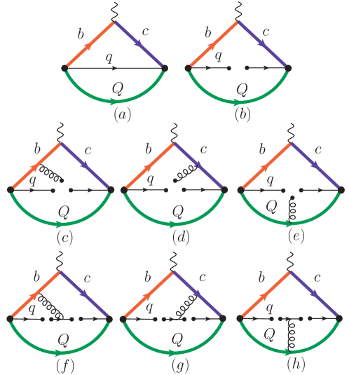
The spectral density of the perturbative diagram in Fig. 1(a) can be obtained as
| (16) | |||||
with
| (17) |
The integral in Eq. (16) can be written as a two-body phase space integral followed by a “triangle” phase space integral Shi:2019hbf .
Equating Eq. (15) with Eq. (12), assuming quark-hadron duality, and performing the Borel transformation, one can obtain
| (18) |
where the left-hand side denotes the Borel transformed four pole terms in Eq. (12) and are the continuum threshold parameters. Equating the coefficients of the same Dirac structures on both sides of Eq. (18), one can arrive at 12 equations, from which, one can further extract the form factors. More details can be found in Shi:2019hbf ; Zhao:2020mod .
In addition, similar as the situation of the two-point correlation function, the LL corrections are also considered.
III Numerical results
The masses of negative-parity baryons are used in this work, and we adopt the results from Wang:2010it ; Roberts:2007ni , which are collected in Table 1.
| Baryon | ||||||
|---|---|---|---|---|---|---|
| Mass | 3.77 | 3.91 | 7.231 | 7.346 | 10.38 | 10.53 |
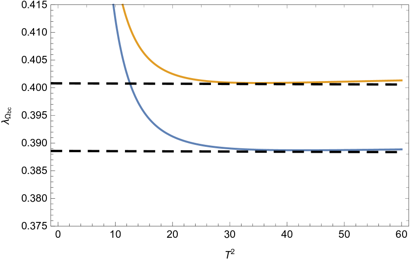
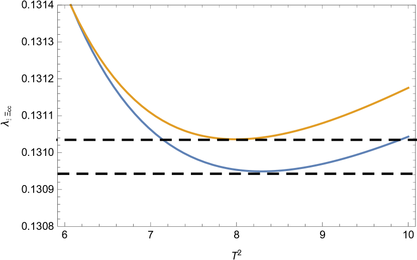
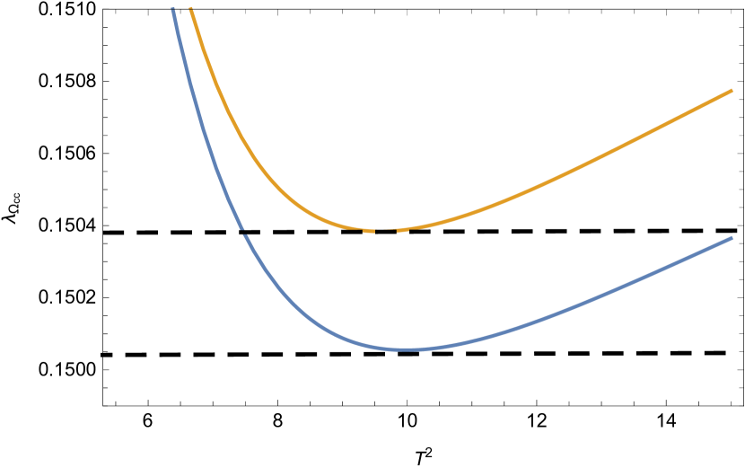
III.1 Pole residues
Our predictioins of pole residues and masses are respectively collected in Table 2 and Table 3, and the pole residues as functions of the Borel parameters are plotted in Fig 2. Both of the results without and with the LL corrections are shown. In Table 3, our predictions for the masses are also compared with those from Lattice QCD Brown:2014ena .
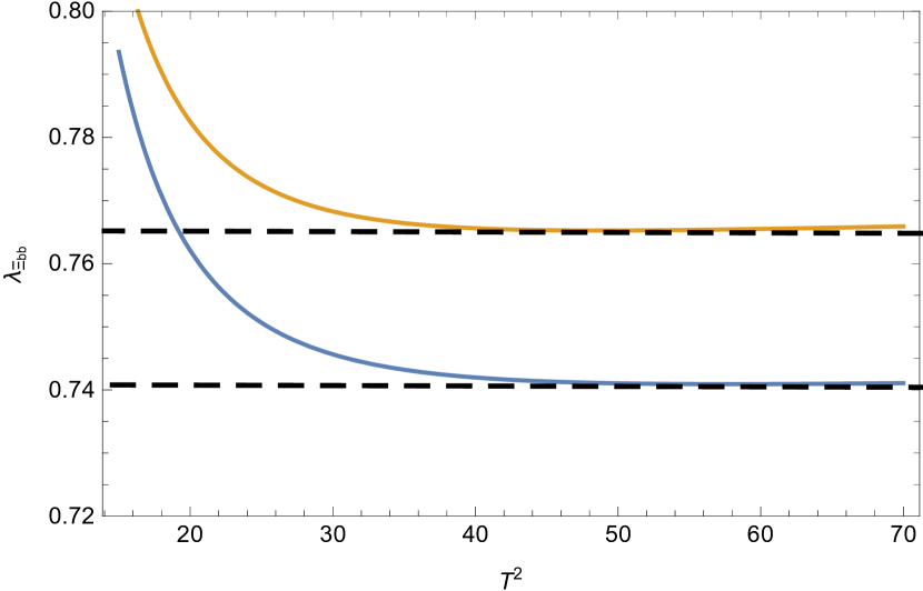
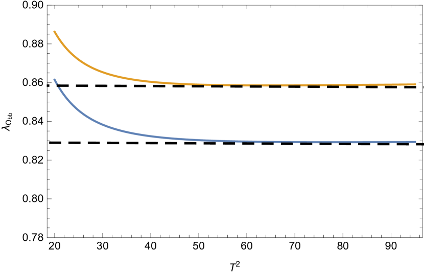
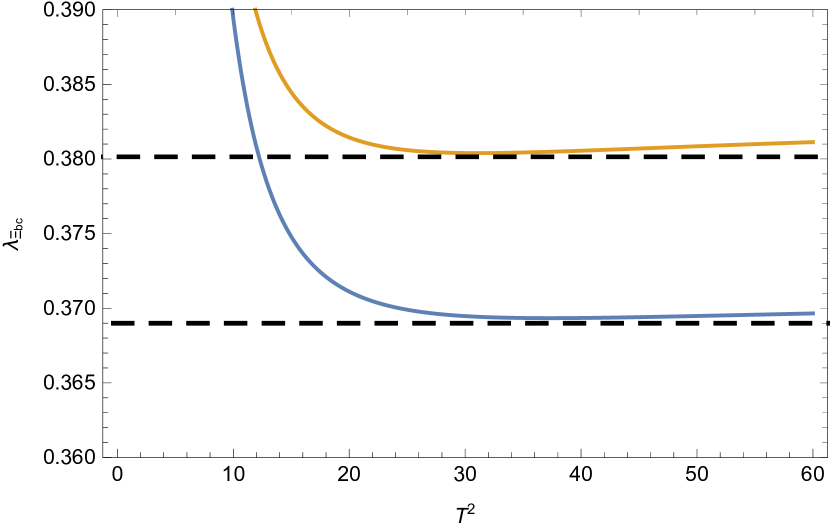
| This work (without the LL corrections) | This work (with the LL corrections) | |
|---|---|---|
| 0.760 | ||
| 0.854 | ||
| 0.379 | ||
| 0.400 | ||
| 0.130 | ||
| 0.150 |
| This work (without the LL corrections) | This work (with the LL corrections) | Lattice QCD Brown:2014ena | |
|---|---|---|---|
| 10.166 | 10.143 | ||
| 10.291 | 10.273 | ||
| 6.948 | 6.943 | ||
| 7.002 | 6.998 | ||
| 3.634 | 3.621 LHCb:2017iph | ||
| 3.747 | 3.738 |
III.2 Form factors
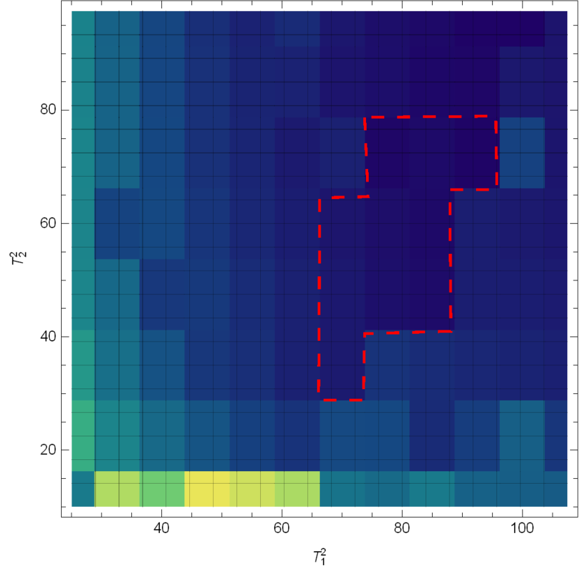
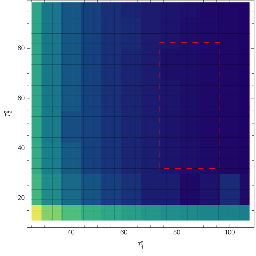
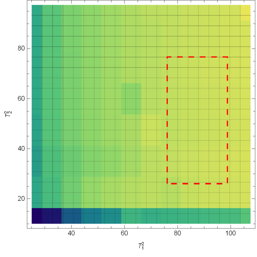
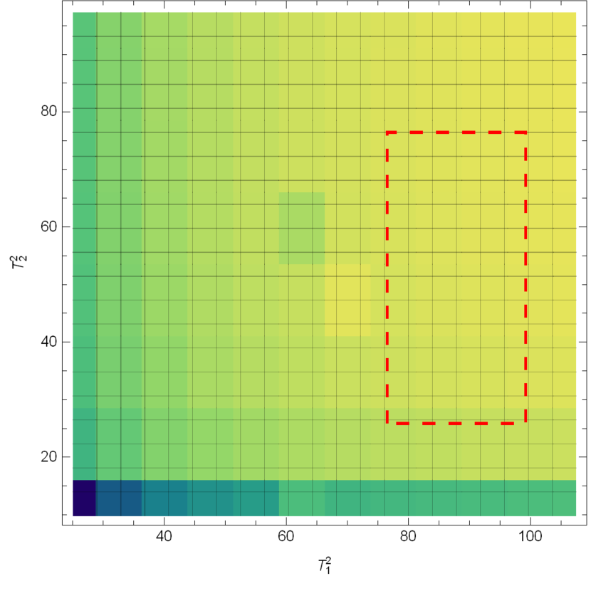
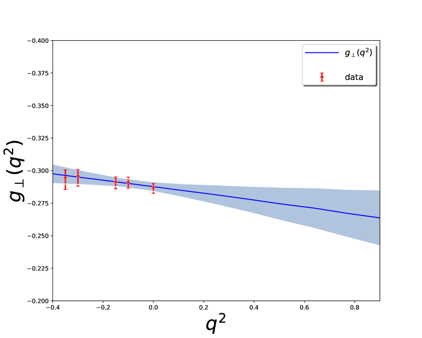
We take the process of as an example to illustrate the selection of Borel windows. In Fig. 3, the transition form factors of are plotted as functions of the Borel parameters . Relatively flat regions are selected as the working Borel windows.
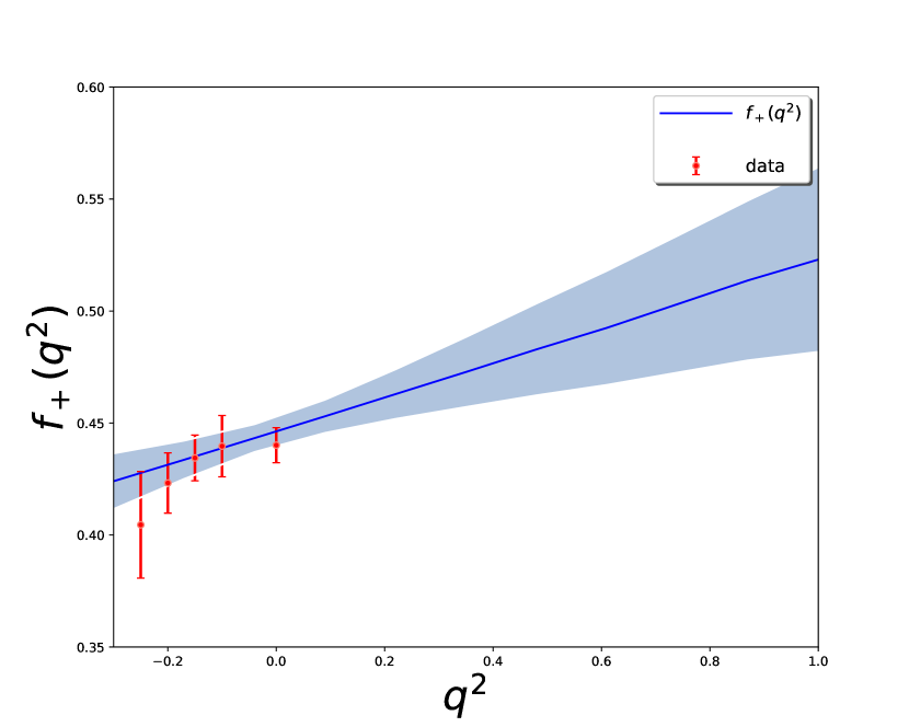
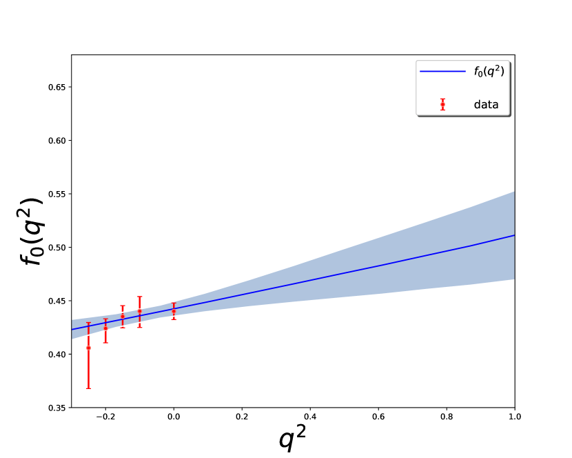
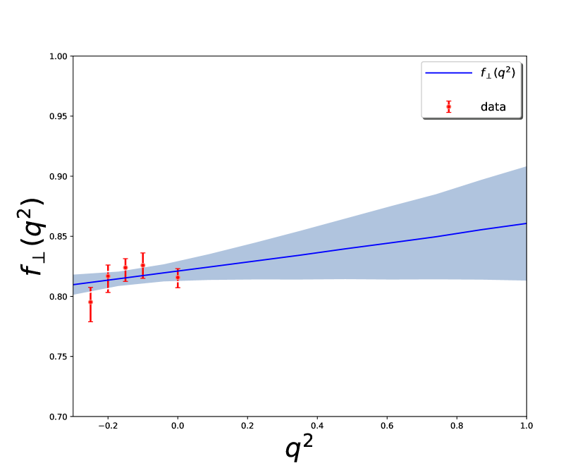
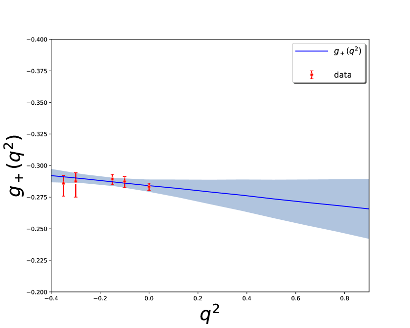
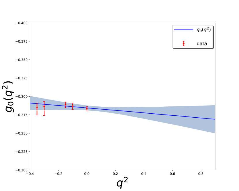
We also consider the uncertainties of the form factors caused by the Borel parameters and the continuum threshold parameter , as can be seen in Table 4. To access the dependence, we calculate the form factors at small , and then fit the data with the following formula
| (19) |
with
| (20) |
Here and are chosen to be equal or below the location of any remaining singularity after factoring out the leading pole contribution Detmold:2015aaa . The nonlinear least- (lsq) method is used in our analysis Peter:2020 . The fitted results are shown in Table 4 and Fig. 4. The contributions of each local operator in the OPE are evaluated as
| (21) |
It can be seen that the OPE has excellent convergence and the perturbative term dominates.
In addition, we have investigated the heavy quark limit of our full QCD results for the form factors, and close results are obtained.
IV Phenomenological applications
The weak decays of doubly heavy baryons induced by can be calculated using the low energy effective Hamiltonian
| (22) |
The helicity amplitudes are defined as follows:
| (23) | |||||
The differential decay widths can be shown as:
| (24) |
Here is the magnitude of three-momentum of in the rest frame of , and is that of lepton in the rest frame of boson. The helicity amplitudes in Eq. (24) are related to the form factors as follows:
| (25) |
and
| (26) |
Our predictions of the decay widths are given in Table 5.
| channel | decay width() |
|---|---|
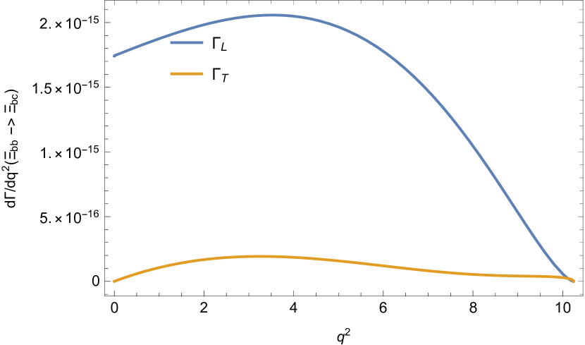
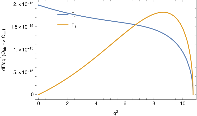
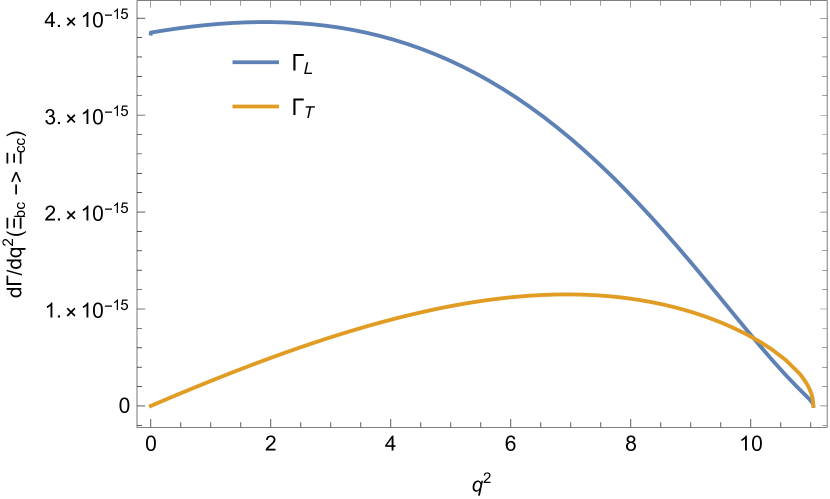
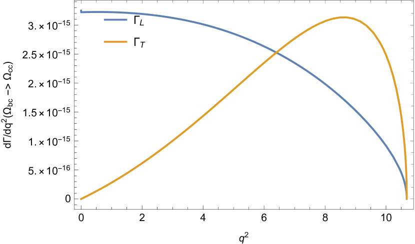
The differential decay widths are plotted in Fig. 5.
V Summary
In this work, we have investigated the decay form factors of doubly heavy baryons in QCD sum rules. For completeness, we have also performed the analysis of pole residues, and as by-products, the masses of doubly heavy baryons. Our predictions for the masses are in good agreement with those of Lattice QCD and experimental data. On the OPE side, contributions from up to dimension-5 and dimension-6 operators are respectively considered for the two-point and three-point correlation functions. We have also considered the leading logarithmic corrections for the Wilson coefficients of OPE, and it turns out that these corrections are small. The obtained form factors are then used to predict the corresponding semi-leptonic decay widths, which are considered to be helpful to search for other doubly heavy baryons at the LHC.
Acknowledgements
The authors would like to thank Prof. Wei Wang for constant help and encouragement. Z.-X. Zhao is supported in part by scientific research start-up fund for Junma program of Inner Mongolia University, scientific research start-up fund for talent introduction in Inner Mongolia Autonomous Region, and National Natural Science Foundation of China under Grant No. 12065020.
References
- (1) R. Aaij et al. [LHCb], Phys. Rev. Lett. 119, no.11, 112001 (2017) doi:10.1103/PhysRevLett.119.112001 [arXiv:1707.01621 [hep-ex]].
- (2) F. S. Yu, H. Y. Jiang, R. H. Li, C. D. Lü, W. Wang and Z. X. Zhao, Chin. Phys. C 42, no.5, 051001 (2018) doi:10.1088/1674-1137/42/5/051001 [arXiv:1703.09086 [hep-ph]].
- (3) A. V. Luchinsky and A. K. Likhoded, Phys. Rev. D 102, no.1, 014019 (2020) doi:10.1103/PhysRevD.102.014019 [arXiv:2007.04010 [hep-ph]].
- (4) A. S. Gerasimov and A. V. Luchinsky, Phys. Rev. D 100, no.7, 073015 (2019) doi:10.1103/PhysRevD.100.073015 [arXiv:1905.11740 [hep-ph]].
- (5) W. Wang, F. S. Yu and Z. X. Zhao, Eur. Phys. J. C 77, no.11, 781 (2017) doi:10.1140/epjc/s10052-017-5360-1 [arXiv:1707.02834 [hep-ph]].
- (6) L. Meng, N. Li and S. l. Zhu, Eur. Phys. J. A 54, no.9, 143 (2018) doi:10.1140/epja/i2018-12578-2 [arXiv:1707.03598 [hep-ph]].
- (7) T. Gutsche, M. A. Ivanov, J. G. Körner and V. E. Lyubovitskij, Phys. Rev. D 96, no.5, 054013 (2017) doi:10.1103/PhysRevD.96.054013 [arXiv:1708.00703 [hep-ph]].
- (8) L. Y. Xiao, K. L. Wang, Q. f. Lu, X. H. Zhong and S. L. Zhu, Phys. Rev. D 96, no.9, 094005 (2017) doi:10.1103/PhysRevD.96.094005 [arXiv:1708.04384 [hep-ph]].
- (9) Q. F. Lü, K. L. Wang, L. Y. Xiao and X. H. Zhong, Phys. Rev. D 96, no.11, 114006 (2017) doi:10.1103/PhysRevD.96.114006 [arXiv:1708.04468 [hep-ph]].
- (10) L. Y. Xiao, Q. F. Lü and S. L. Zhu, Phys. Rev. D 97, no.7, 074005 (2018) doi:10.1103/PhysRevD.97.074005 [arXiv:1712.07295 [hep-ph]].
- (11) Z. X. Zhao, Eur. Phys. J. C 78, no.9, 756 (2018) doi:10.1140/epjc/s10052-018-6213-2 [arXiv:1805.10878 [hep-ph]].
- (12) Z. P. Xing and Z. X. Zhao, Phys. Rev. D 98, no.5, 056002 (2018) doi:10.1103/PhysRevD.98.056002 [arXiv:1807.03101 [hep-ph]].
- (13) R. Dhir and N. Sharma, Eur. Phys. J. C 78, no.9, 743 (2018) doi:10.1140/epjc/s10052-018-6220-3
- (14) L. J. Jiang, B. He and R. H. Li, Eur. Phys. J. C 78, no.11, 961 (2018) doi:10.1140/epjc/s10052-018-6445-1 [arXiv:1810.00541 [hep-ph]].
- (15) T. Gutsche, M. A. Ivanov, J. G. Körner, V. E. Lyubovitskij and Z. Tyulemissov, Phys. Rev. D 99, no.5, 056013 (2019) doi:10.1103/PhysRevD.99.056013 [arXiv:1812.09212 [hep-ph]].
- (16) T. Gutsche, M. A. Ivanov, J. G. Körner and V. E. Lyubovitskij, Particles 2, no.2, 339-356 (2019) doi:10.3390/particles2020021 [arXiv:1905.06219 [hep-ph]].
- (17) Q. X. Yu, J. M. Dias, W. H. Liang and E. Oset, Eur. Phys. J. C 79, no.12, 1025 (2019) doi:10.1140/epjc/s10052-019-7543-4 [arXiv:1909.13449 [hep-ph]].
- (18) T. Gutsche, M. A. Ivanov, J. G. Körner, V. E. Lyubovitskij and Z. Tyulemissov, Phys. Rev. D 100, no.11, 114037 (2019) doi:10.1103/PhysRevD.100.114037 [arXiv:1911.10785 [hep-ph]].
- (19) A. V. Berezhnoy, A. K. Likhoded and A. V. Luchinsky, J. Phys. Conf. Ser. 1390, no.1, 012031 (2019) doi:10.1088/1742-6596/1390/1/012031
- (20) H. W. Ke, F. Lu, X. H. Liu and X. Q. Li, Eur. Phys. J. C 80, no.2, 140 (2020) doi:10.1140/epjc/s10052-020-7699-y [arXiv:1912.01435 [hep-ph]].
- (21) H. Y. Cheng, G. Meng, F. Xu and J. Zou, Phys. Rev. D 101, no.3, 034034 (2020) doi:10.1103/PhysRevD.101.034034 [arXiv:2001.04553 [hep-ph]].
- (22) X. H. Hu, R. H. Li and Z. P. Xing, Eur. Phys. J. C 80, no.4, 320 (2020) doi:10.1140/epjc/s10052-020-7851-8 [arXiv:2001.06375 [hep-ph]].
- (23) S. Rahmani, H. Hassanabadi and H. Sobhani, Eur. Phys. J. C 80, no.4, 312 (2020) doi:10.1140/epjc/s10052-020-7867-0
- (24) M. A. Ivanov, J. G. Körner and V. E. Lyubovitskij, Phys. Part. Nucl. 51, no.4, 678-685 (2020) doi:10.1134/S1063779620040358
- (25) R. H. Li, J. J. Hou, B. He and Y. R. Wang, doi:10.1088/1674-1137/abe0bc [arXiv:2010.09362 [hep-ph]].
- (26) J. J. Han, R. X. Zhang, H. Y. Jiang, Z. J. Xiao and F. S. Yu, Eur. Phys. J. C 81, no.6, 539 (2021) doi:10.1140/epjc/s10052-021-09239-w [arXiv:2102.00961 [hep-ph]].
- (27) W. Wang, Z. P. Xing and J. Xu, Eur. Phys. J. C 77, no.11, 800 (2017) doi:10.1140/epjc/s10052-017-5363-y [arXiv:1707.06570 [hep-ph]].
- (28) Y. J. Shi, W. Wang, Y. Xing and J. Xu, Eur. Phys. J. C 78, no.1, 56 (2018) doi:10.1140/epjc/s10052-018-5532-7 [arXiv:1712.03830 [hep-ph]].
- (29) Q. A. Zhang, Eur. Phys. J. C 78, no.12, 1024 (2018) doi:10.1140/epjc/s10052-018-6481-x [arXiv:1811.02199 [hep-ph]].
- (30) H. S. Li, L. Meng, Z. W. Liu and S. L. Zhu, Phys. Lett. B 777, 169-176 (2018) doi:10.1016/j.physletb.2017.12.031 [arXiv:1708.03620 [hep-ph]].
- (31) A. V. Berezhnoy, A. K. Likhoded and A. V. Luchinsky, Phys. Rev. D 98, no.11, 113004 (2018) doi:10.1103/PhysRevD.98.113004 [arXiv:1809.10058 [hep-ph]].
- (32) Z. H. Guo, Phys. Rev. D 96, no.7, 074004 (2017) doi:10.1103/PhysRevD.96.074004 [arXiv:1708.04145 [hep-ph]].
- (33) Y. L. Ma and M. Harada, J. Phys. G 45, no.7, 075006 (2018) doi:10.1088/1361-6471/aac86e [arXiv:1709.09746 [hep-ph]].
- (34) X. Yao and B. Müller, Phys. Rev. D 97, no.7, 074003 (2018) doi:10.1103/PhysRevD.97.074003 [arXiv:1801.02652 [hep-ph]].
- (35) D. L. Yao, Phys. Rev. D 97, no.3, 034012 (2018) doi:10.1103/PhysRevD.97.034012 [arXiv:1801.09462 [hep-ph]].
- (36) L. Meng and S. L. Zhu, Phys. Rev. D 100, no.1, 014006 (2019) doi:10.1103/PhysRevD.100.014006 [arXiv:1811.07320 [hep-ph]].
- (37) Y. J. Shi, W. Wang, Z. X. Zhao and U. G. Meißner, Eur. Phys. J. C 80, no.5, 398 (2020) doi:10.1140/epjc/s10052-020-7949-z [arXiv:2002.02785 [hep-ph]].
- (38) P. C. Qiu and D. L. Yao, Phys. Rev. D 103, no.3, 034006 (2021) doi:10.1103/PhysRevD.103.034006 [arXiv:2012.11117 [hep-ph]].
- (39) A. R. Olamaei, K. Azizi and S. Rostami, [arXiv:2102.03852 [hep-ph]].
- (40) Q. Qin, Y. J. Shi, W. Wang, Y. Guo-He, F. S. Yu and R. Zhu, [arXiv:2108.06716 [hep-ph]].
- (41) X. H. Hu, Y. L. Shen, W. Wang and Z. X. Zhao, Chin. Phys. C 42, no.12, 123102 (2018) doi:10.1088/1674-1137/42/12/123102 [arXiv:1711.10289 [hep-ph]].
- (42) R. H. Li and C. D. Lu, [arXiv:1805.09064 [hep-ph]].
- (43) Y. J. Shi, W. Wang and Z. X. Zhao, Eur. Phys. J. C 80, no.6, 568 (2020) doi:10.1140/epjc/s10052-020-8096-2 [arXiv:1902.01092 [hep-ph]].
- (44) E. L. Cui, H. X. Chen, W. Chen, X. Liu and S. L. Zhu, Phys. Rev. D 97, no.3, 034018 (2018) doi:10.1103/PhysRevD.97.034018 [arXiv:1712.03615 [hep-ph]].
- (45) Y. J. Shi, Y. Xing and Z. X. Zhao, Eur. Phys. J. C 79, no.6, 501 (2019) doi:10.1140/epjc/s10052-019-7014-y [arXiv:1903.03921 [hep-ph]].
- (46) X. H. Hu and Y. J. Shi, Eur. Phys. J. C 80, no.1, 56 (2020) doi:10.1140/epjc/s10052-020-7635-1 [arXiv:1910.07909 [hep-ph]].
- (47) A. R. Olamaei, K. Azizi and S. Rostami, Eur. Phys. J. C 80, no.7, 613 (2020) doi:10.1140/epjc/s10052-020-8194-1 [arXiv:2003.12723 [hep-ph]].
- (48) H. I. Alrebdi, T. M. Aliev and K. Şimşek, Phys. Rev. D 102, no.7, 074007 (2020) doi:10.1103/PhysRevD.102.074007 [arXiv:2008.05098 [hep-ph]].
- (49) S. Rostami, K. Azizi and A. R. Olamaei, Chin. Phys. C 45, no.2, 023120 (2021) doi:10.1088/1674-1137/abd084 [arXiv:2008.12715 [hep-ph]].
- (50) T. M. Aliev and K. Şimşek, Eur. Phys. J. C 80, no.10, 976 (2020) doi:10.1140/epjc/s10052-020-08553-z [arXiv:2009.03464 [hep-ph]].
- (51) T. M. Aliev, T. Barakat and K. Şimşek, Eur. Phys. J. A 57, no.5, 160 (2021) doi:10.1140/epja/s10050-021-00471-2 [arXiv:2101.10264 [hep-ph]].
- (52) K. Azizi, A. R. Olamaei and S. Rostami, Eur. Phys. J. C 80, no.12, 1196 (2020) doi:10.1140/epjc/s10052-020-08770-6 [arXiv:2011.02919 [hep-ph]].
- (53) F. S. Yu, Sci. China Phys. Mech. Astron. 63, no.2, 221065 (2020) doi:10.1007/s11433-019-1483-0 [arXiv:1912.10253 [hep-ex]].
- (54) T. Feldmann and M. W. Y. Yip, Phys. Rev. D 85, 014035 (2012) [erratum: Phys. Rev. D 86, 079901 (2012)] doi:10.1103/PhysRevD.85.014035 [arXiv:1111.1844 [hep-ph]].
- (55) Z. X. Zhao, Y. J. Shi and Z. P. Xing, [arXiv:2104.06209 [hep-ph]].
- (56) E. V. Shuryak, Nucl. Phys. B 198, 83-101 (1982) doi:10.1016/0550-3213(82)90546-6
- (57) R. S. Marques de Carvalho, F. S. Navarra, M. Nielsen, E. Ferreira and H. G. Dosch, Phys. Rev. D 60, 034009 (1999) doi:10.1103/PhysRevD.60.034009 [arXiv:hep-ph/9903326 [hep-ph]].
- (58) Z. X. Zhao, R. H. Li, Y. J. Shi and S. H. Zhou, [arXiv:2005.05279 [hep-ph]].
- (59) A. J. Buras, [arXiv:hep-ph/9806471 [hep-ph]].
- (60) Z. X. Zhao, R. H. Li, Y. L. Shen, Y. J. Shi and Y. S. Yang, Eur. Phys. J. C 80, no.12, 1181 (2020) doi:10.1140/epjc/s10052-020-08767-1 [arXiv:2010.07150 [hep-ph]].
- (61) Z. G. Wang, Eur. Phys. J. C 78, no.10, 826 (2018) doi:10.1140/epjc/s10052-018-6300-4 [arXiv:1808.09820 [hep-ph]].
- (62) Z. G. Wang, Eur. Phys. J. A 47, 81 (2011) doi:10.1140/epja/i2011-11081-8 [arXiv:1003.2838 [hep-ph]].
- (63) W. Roberts and M. Pervin, Int. J. Mod. Phys. A 23, 2817-2860 (2008) doi:10.1142/S0217751X08041219 [arXiv:0711.2492 [nucl-th]].
- (64) Z. S. Brown, W. Detmold, S. Meinel and K. Orginos, Phys. Rev. D 90, no.9, 094507 (2014) doi:10.1103/PhysRevD.90.094507 [arXiv:1409.0497 [hep-lat]].
- (65) W. Detmold, C. Lehner and S. Meinel, Phys. Rev. D 92, no.3, 034503 (2015) doi:10.1103/PhysRevD.92.034503 [arXiv:1503.01421 [hep-lat]].
- (66) P. Lepage and C. Gohlke, gplepage/lsqfit: lsqfit version 11.7, Zenodo. http://doi.org/10.5281/zenodo.4037174