Pyramid Adversarial Training Improves ViT Performance

Charles Herrmann Kyle Sargent^* Lu Jiang Ramin Zabih
Huiwen Chang Ce Liu Dilip Krishnan Deqing Sun
Google Research Equal contribution, ordered alphabetically.Currently affiliated with Microsoft Azure AI.

Abstract

Aggressive data augmentation is a key component of the strong generalization capabilities of Vision Transformer (ViT). One such data augmentation technique is adversarial training (AT); however, many prior works[45, 28] have shown that this often results in poor clean accuracy. In this work, we present pyramid adversarial training (PyramidAT), a simple and effective technique to improve ViT’s overall performance. We pair it with a “matched” Dropout and stochastic depth regularization, which adopts the same Dropout and stochastic depth configuration for the clean and adversarial samples. Similar to the improvements on CNNs by AdvProp [61] (not directly applicable to ViT), our pyramid adversarial training breaks the trade-off between in-distribution accuracy and out-of-distribution robustness for ViT and related architectures. It leads to $1.82\%$ absolute improvement on ImageNet clean accuracy for the ViT-B model when trained only on ImageNet-1K data, while simultaneously boosting performance on $7$ ImageNet robustness metrics, by absolute numbers ranging from $1.76\%$ to $15.68\%$ . We set a new state-of-the-art for ImageNet-C (41.42 mCE), ImageNet-R (53.92%), and ImageNet-Sketch (41.04%) without extra data, using only the ViT-B/16 backbone and our pyramid adversarial training. Our code is publicly available at pyramidat.github.io.

1 Introduction

One fascinating aspect of human intelligence is the ability to generalize from limited experiences to new environments [30]. While deep learning has made remarkable progress in emulating or “surpassing” humans on classification tasks, deep models have difficulty generalizing to out-of-distribution data [31]. Convolutional neural networks (CNNs) may fail to classify images with challenging contexts [22], unusual colors and textures [19, 58, 16] and common or adversarial corruptions [20, 17]. To reliably deploy neural networks on diverse tasks in the real world, we must improve their robustness to out-of-distribution data.

Refer to caption — Figure 1: Top: Visualization of our learned multi-scale pyramid perturbations. We show the original image, multiple scales of a perturbation pyramid, and the perturbed image. Bottom: We show thumbnails of in-distribution and out-of-distribution datasets, and the gains from applying our technique on each dataset. (Note that lower is better for ImageNet-C.)

One major line of research focuses on network design. Recently the Vision Transformer (ViT) [15] and its variants [55, 32, 46, 2] have advanced the state of the art on a variety of computer vision tasks. In particular, ViT models are more robust than comparable CNN architectures [38, 49, 49, 36]. With a weak inductive bias and powerful model capacity, ViT relies heavily on strong data augmentation and regularization to achieve better generalization [51, 55]. To further push this envelope, we explore using adversarial training [29, 65] as a powerful regularizer to improve the performance of ViT models.

Prior work [56] suggests that there exists a performance trade-off between in-distribution generalization and robustness to adversarial examples. Similar trade-offs have been observed between in-distribution and out-of-distribution generalization [45, 65]. These trade-offs have primarily been observed in the context of CNNs [7, 45]. However, recent work has demonstrated the trade-off can be broken. AdvProp [61] achieves this via adversarial training (abbreviated AT) with a “split” variant of Batch Normalization [24] for EfficientNet [53]. In our work, we demonstrate that the trade-off can be broken for the newly introduced vision transformer architecture [15].

We introduce pyramid adversarial training (abbreviated as PyramidAT) that trains the model with input images altered at multiple spatial scales, as illustrated in Fig. 1; the pyramid attack is designed to make large edits to the image in a structured, controlled manner (similar to augmenting brightness) and small edits to the image in a flexible manner (similar to pixel adversaries). Using these structured, multi-scale adversarial perturbations leads to significant performance gains compared to both baseline and standard pixel-wise adversarial perturbations. Interestingly, we see these gains for both clean (in-distribution) and robust (out-of-distribution) accuracy. We further enhance the pyramid attack with additional regularization techniques: “matched” Dropout and stochastic depth. Matched Dropout uses the same Dropout configuration for both the regular and adversarial samples in a mini-batch (hence the word matched). Stochastic depth [23, 51] randomly drops layers in the network and provides a further boost when matched and paired with matched Dropout and multi-scale perturbations.

Our ablation studies confirm the importance of matched Dropout when used in conjunction with the pyramid adversarial training. They also reveal a complicated interplay between adversarial training, the attack being used, and network capacity. We additionally show that our approach is applicable to datasets of various scales (ImageNet-1K and ImageNet-21K) and for a variety of network architectures such as ViT [15], Discrete ViT [37], ResNet[18], and MLP-Mixer [54]. Our contributions are summarized below:

•

To our knowledge, we appear to be the first to demonstrate that adversarial training improves ViT model performance on both ImageNet [13] and out-of-distribution ImageNet robustness datasets [22, 20, 19, 58, 16].
•

We demonstrate the importance of matched Dropout and stochastic depth for the adversarial training of ViT.
•

We design pyramid adversarial training to generate multi-scale, structured adversarial perturbations, which achieve significant performance gains over non-adversarial baseline and adversarial training with pixel perturbations.
•

We establish a new state of the art for ImageNet-C, ImageNet-R, and ImageNet-Sketch without extra data, using only our pyramid adversarial training and the standard ViT-B/16 backbone. We further improve our results by incorporating extra ImageNet-21K data.
•

We perform numerous ablations which highlight several elements critical to the performance gains.

2 Related Work

There exists a large body of work on measuring and improving the robustness of deep learning models, in the context of adversarial examples and generalization to non-adversarial but shifted distributions. We define out-of-distribution accuracy/robustness to explicitly refer to performance of a model on non-adversarial distribution shifts, and adversarial accuracy/robustness to refer to the special case of robustness on adversarial examples. When the evaluation is performed on a dataset drawn from the same distribution, we call this clean accuracy.

Adversarial training and robustness

The discovery of adversarial examples [52] has stimulated a large body of literature on adversarial attacks and defenses [29, 35, 40, 44, 1, 6, 43, 60]. Of the many proposed defenses, adversarial training [29, 35] has emerged as a simple, effective, albeit expensive approach to make networks adversarially robust. Although some work [56, 65] has suggested a tradeoff between adversarial and out-of-distribution robustness or clean accuracy, other analysis [7, 45] has suggested simultaneous improvement is achievable. In [45, 39], the authors note improved accuracy on both clean and adversarially perturbed data, though only on smaller datasets such as CIFAR-10 [27] and SVHN [42], and only through the use of additional data extending the problem to the semi-supervised setting. Similarly in NLP, adversarial training leads to improvement of clean accuracy for machine translation [9, 8].

Most closely related to our work is the technique of [61], which demonstrates the potential of adversarial training to improve both clean accuracy and out-of-distribution robustness. They focus primarily on CNNs and propose split batch norms to separately capture the statistics of clean and adversarially perturbed samples in a mini-batch. At inference time, the batch norms associated with adversarially perturbed samples are discarded, and all data (presumed clean or out-of-distribution) flows through the batch norms associated with clean samples. Their results are demonstrated on EfficientNet[53] and ResNet [18] architectures. However, their approach is not directly applicable to ViT where batch norms do not exist. In our work, we propose novel approaches, and find that properly constructed adversarial training helps clean accuracy and out-of-distribution robustness for ViT models.

Robustness of ViT

ViT models have been found to be more adversarially robust than CNNs [49, 41], and more importantly, generalize better than CNNs with similar model capacity on ImageNet out-of-distribution robustness benchmarks [49]. While existing works focus on analyzing the cause of ViT’s superior generalizability, this work aims at further improving the strong out-of-distribution robustness of the ViT model. A promising approach to this end is data augmentation; as shown recently [51, 55], ViT benefits from strong data augmentation. However, the data augmentation techniques used in ViT [51, 55] are optimized for clean accuracy on ImageNet, and knowledge about robustness is still limited. Different from prior works, this paper focuses on improving both the clean accuracy and robustness for ViT. We show that our technique can effectively complement strong ViT augmentation as in [51]. We additionally verify that our proposed augmentation can benefit three other architectures: ResNet[18], MLP-Mixer [54], and Discrete ViT [37].

Data augmentation

Existing data augmentation techniques, although mainly developed for CNNs, transfer reasonably well to ViT models [10, 59, 21]. Other work has studied larger structured attacks [60]. Our work is different from prior work in that we utilize adversarial training to augment ViT and tailor our design to the ViT architecture. To our knowledge, we appear to be the first to demonstrate that adversarial training substantially improves ViT performance in both clean and out-of-distribution accuracies.

3 Approach

We work in the supervised learning setting where we are given a training dataset $\mathcal{D}$ consisting of clean images, represented as $x$ and their labels $y$ . The loss function considered is a cross-entropy loss $L(\theta,x,y)$ , where $\theta$ are the parameters of the ViT model, with weight regularization $f$ . The baseline models minimize the following loss:

\mathbb{E}_{(x,y)\sim\mathcal{D}}\Big{[}L(\theta,\tilde{x},y)+f(\theta)\Big{]},

(1)

where $\tilde{x}$ refers to a data-augmented version of the clean sample $x$ , and we adopt the standard data augmentations as in [51], such as RandAug [10].

3.1 Adversarial Training

The overall training objective for adversarial training [57] is given as follows:

\mathbb{E}_{(x,y)\sim\mathcal{D}}\Big{[}\max_{\delta\in\mathcal{P}}L(\theta,\tilde{x}+\delta,y)+f(\theta)\Big{]},

(2)

where $\delta$ a per-pixel, per-color-channel additive perturbation, and $\mathcal{P}$ is the perturbation distribution. Note that the adversarial image, $x^{a}$ , is given by $\tilde{x}+\delta$ , and we use these two interchangeably below. The perturbation, $\delta$ , is computed by optimizing the objective inside the maximization of Eqn. 2. This objective tries to improve the worst-case performance of the network w.r.t. the perturbation; subsequently, the resulting model has lower clean accuracy.

To remedy this, we can train on both clean and adversarial images [17, 29, 61] using the following objective:

\mathbb{E}_{(x,y)\sim\mathcal{D}}\Big{[}L(\theta,\tilde{x},y)+\lambda\max_{\delta\in\mathcal{P}}L(\theta,\tilde{x}+\delta,y)+f(\theta)\Big{]},

(3)

This objective uses adversarial images as a form of regularization or data augmentation, to force the network towards certain representations that perform well on out-of-distribution data. These networks exhibit some degree of robustness but still have good clean accuracy. More recently, [61] proposes a split batch norm that leads to performance gains for CNNs on both clean and robust ImageNet test datasets. Note that they do not concern themselves with adversarial robustness, and neither do we in this paper.

3.2 Pyramid Adversarial Training

Pixel-wise adversarial images are defined[29] as $x^{a}=x+\delta$ where the perturbation distribution $P$ consists of a clipping function $C_{\mathcal{B}_{\epsilon}}$ that clips the perturbation at each pixel location to be inside the specified ball ( $\mathcal{B}_{\epsilon}$ ) for a specified $l_{p}$ -norm [35], with maximal radius $\epsilon$ for the perturbation.

Motivation

For pixel-wise adversarial images, increasing the value of $\epsilon$ or the number of steps of the inner loop in Eqn. 3 eventually causes a drop in clean accuracy (Fig 2). Conceptually, pixel attacks are very flexible and, if given the ability to make large changes (in $L_{2}$ distance), can destroy the object being classified; training with these images may harm the network. In contrast, augmentations, like brightness, can lead to large $L_{2}$ distances but will preserve the object because they are structured. Our main motivation is to design an attack which has the best of both worlds: a low-magnitude flexible component and a high-magnitude structured component; this attack can lead to large image differences while still preserving the class identity.

Approach

We propose pyramid adversarial training (PyramidAT) which generates adversarial examples by perturbing the input image at multiple scales. This attack is more flexible and yet also more structured, since it consists of multiple scales, but the perturbations are constrained at each scale.

x^{a}=C_{\mathcal{B}_{1}}\Big{(}\tilde{x}+\sum_{s\in S}m_{s}\cdot C_{\mathcal{B}_{\epsilon_{s}}}(\delta_{s})\Big{)},

(4)

where $C_{\mathcal{B}_{1}}$ is the clipping function that keeps the image within the normal range, $S$ is the set of scales, $m_{s}$ is the multiplicative constant for scale $s$ , $\delta_{s}$ is the learned perturbation (with the same shape as $x$ ). For scale $s$ , the weights in $\delta_{s}$ are shared for pixels in square regions of size $s\times s$ with top left corner $[s\cdot i,s\cdot j]$ for all discrete $i\in[0,\textrm{width}/s]$ and $j\in[0,\textrm{height}/s]$ , as shown in Fig. 1. Note that, similar to pixel AT, each channel of the image is perturbed independently. More details of the parameter settings are given in Section 4 and pseudocode is included in the supplementals.

Setting up the attack

For both the pixel and pyramid attacks, we use Projected Gradient Descent (PGD) on a random label using multiple steps [35]. With regards to the loss, we observe that for ViT, maximizing the negative loss of the true label leads to aggressive label leaking [29], i.e., the network learns to predict the adversarial attack and performs better on the perturbed image. To avoid this, we pick a random label and then minimize the softmax cross-entropy loss towards that random label as described in [29].

3.3 “Matched” Dropout and Stochastic Depth

Standard training for ViT models uses both Dropout [50] and stochastic depth [23] as regularizers. During adversarial training, we have both the clean samples and adversarial samples in a mini-batch. This poses a question about Dropout treatment during adversarial training (either pixel or pyramid). In the adversarial training literature, the usual strategy is to run the adversarial attack (to generate adversarial samples) without using Dropout or stochastic depth. However, this leads to a training mismatch between the clean and adversarial training paths when both are used in the loss (Eqn. 3), with the clean samples trained with Dropout and the adversarial samples without Dropout. For each training instance in the mini-batch, the clean branch will only update subsets of the network while the adversarial branch updates the entire network. The adversarial branch updates are therefore more closely aligned with the model performance during evaluation, thereby leading to an improvement of adversarial accuracy at the expense of clean accuracy. This objective function is given below:

\mathbb{E}_{(x,y)\sim\mathcal{D}}\Big{[}L(\mathcal{M}(\theta),\tilde{x},y)+\lambda\max_{\delta\in\mathcal{P}}L(\theta,x^{a},y)+f(\theta)\Big{]},

(5)

where, with a slight abuse of notation, $\mathcal{M}(\theta)$ denotes a network with a random Dropout mask and a stochastic depth configuration. To address the issue above, we propose adversarial training of ViT with “matched” Dropout, i.e., using the same Dropout configuration for both clean and adversarial training branches (as well as for the generation of adversarial samples). We show through ablation in Section 4 that using the same Dropout configuration leads to the best overall performance for both the clean and robust datasets.

4 Experiments

In this section, we compare the effectiveness of our proposed PyramidAT to non-AT models, and PixelAT models.

4.1 Experimental Setup

			Out of Distribution Robustness Test
Method	ImageNet	Real	A	C $\downarrow$	ObjectNet	V2	Rendition	Sketch	Stylized
ViT [15]	72.82	78.28	8.03	74.08	17.36	58.73	27.07	17.28	6.41
ViT+CutMix [63]	75.49	80.53	14.75	64.07	21.61	62.37	28.47	17.15	7.19
ViT+Mixup [64]	77.75	82.93	12.15	61.76	25.65	64.76	34.90	25.97	9.84
RegViT (RandAug) [51]	79.92	85.14	17.48	52.46	29.30	67.49	38.24	29.08	11.02
+Random Pixel	79.72	84.72	17.81	52.83	28.72	67.17	39.01	29.26	12.11
+Random Pyramid	80.06	85.02	19.15	52.49	29.41	67.81	39.78	30.30	11.64
+PixelAT	80.42	85.78	19.15	47.68	30.11	68.78	45.39	34.40	18.28
+PyramidAT (Ours)	81.71	86.82	22.99	44.99	32.92	70.82	47.66	36.77	19.14
RegViT [51] on 384x384	81.44	86.38	26.20	58.19	35.59	70.09	38.15	28.13	8.36
+Random Pixel	81.32	86.18	25.95	58.69	34.12	69.50	37.66	28.79	9.77
+Random Pyramid	81.42	86.30	27.55	57.31	34.83	70.53	38.12	29.16	9.61
+PixelAT	82.24	87.35	31.23	48.56	37.41	71.67	44.07	33.68	13.52
+PyramidAT (Ours)	83.26	88.14	36.41	47.76	39.79	73.14	46.68	36.73	15.00

Table 1: Main results on ImageNet-1k. All columns reports top-1 accuracy except ImageNet-C which reports mean Corruption Error (mCE) where lower is better. All models are ViT-B/16. The first set of rows show the performance on train and testing on

224\times 224

images. The second set of rows shows performance by fine-tuning on

384\times 384

images.

Method	Extra Data	IM-C mCE $\downarrow$
DeepAugment+AugMix [19]	✗	53.60
AdvProp [61]	✗	52.90
Robust ViT [38]	✗	46.80
Discrete ViT [37]	✗	46.20
QualNet [25]	✗	42.50
Ours (ViT-B/16 + PyramidAT)	✗	41.42
Discrete ViT [37]	✓	38.74
Ours (ViT-B/16 + PyramidAT)	✓	36.80

Table 2: Comparison to state of the art for mean Corruption Error (mCE) on ImageNet-C. Extra data is IM-21k.

Method	Extra Data	IM-Rendition
Faces of Robustness [19]	✗	46.80
Robust ViT [38]	✗	48.70
Discrete ViT [37]	✗	48.82
Ours (ViT-B/16 + PyramidAT)	✗	53.92
Discrete ViT [37]	✓	55.26
Ours (ViT-B/16 + PyramidAT)	✓	57.84

Table 3: Comparison to state of the art for Top-1 on ImageNet-R. Extra data is IM-21k.

Method	Extra Data	IM-Sketch
ConViT-B[11]	✗	35.70
Swin-B[32]	✗	32.40
Robust ViT [38]	✗	36.00
Discrete ViT [37]	✗	39.10
Ours (ViT-B/16 + PyramidAT)	✗	41.04
Discrete ViT [37]	✓	44.72
Ours (ViT-B/16 + PyramidAT)	✓	46.03

Table 4: Comparison to state of the art for Top-1 on ImageNet-Sketch. Extra data is IM-21k.

Models

We focus primarily on ViT-B/16 [15], the baseline ViT with a patch size of 16. We also demonstrate our technique on other network architectures, such as ViT-Ti/16, ResNet [18], MLP-Mixer [54], and the recent Discrete ViT [37].

Datasets

We train models on both ImageNet-1K and ImageNet-21K [48, 13]. We evaluate in-distribution performance on 2 additional variants: ImageNet-ReaL [4] which relabels the validation set of the original ImageNet in order to correct labeling errors; and ImageNet-V2[47] which collects another version of ImageNet’s evaluation set. We evaluate out-of-distribution robustness on 6 datasets: ImageNet-A [22] which places the ImageNet objects in unusual contexts or orientations; ImageNet-C [20] which applies a series of corruptions (e.g. motion blur, snow, JPEG, etc.); ImageNet-Rendition [19] which contains abstract or rendered versions of the object; ObjectNet [3] which consists of a large real-world set from a large number of different backgrounds, rotations, and imaging view points; ImageNet-Sketch [58] which contains artistic sketches of the objects; and Stylized ImageNet [16] which processes the ImageNet images with style transfer from an unrelated source image. For brevity, we may abbreviate ImageNet as IM. For all datasets except IM-C, we report top-1 accuracy (where higher is better). For IM-C, we report the standard “Mean corruption error” (mCE) (where lower is better).

Implementation details

Following [51], we use a batch size of 4096, a cosine decay learning rate schedule (0.001 magnitude) with linear warmup for the first 10k steps, [34], and the AdamW optimizer [26] in all our experiments. Augmentations and regularizations include RandAug[10] with the default setting of $(2,15)$ , Dropout [50] at probability $0.1$ , and stochastic depth [23] at probability $0.1$ . We train with Scenic[12], a Jax[5] library, on DragonFish TPUs.

To generate the pixel adversarial attack, we follow [61]. We use a learning rate of $1/255$ , $\epsilon=4/255$ , and attack for $5$ steps with SGD. We use PGD [35] to generate the adversarial perturbations. We also experiment with using more recent optimizers [66] to construct the attacks (results are provided in the supplementals). For pyramid attacks, we find using stronger perturbations at coarser scales is more effective than equal perturbation strengths across all scales. By default, we use a 3-level pyramid and use perturbation scale factors $S=[32,16,1]$ (a scale of $1$ means that each pixel has one learned parameter, a scale of $16$ means that each $[16,16]$ patch has one learned parameter) with multiplicative terms of $m_{s}=[20,10,1]$ (see Eqn. 4). We use a clipping value of $\epsilon_{s}=6/255$ for all levels of the pyramid.

4.2 Experimental Results on ViT-B/16

			Out of Distribution Robustness Test
Method	ImageNet	Real	A	C $\downarrow$	ObjectNet	V2	Rendition	Sketch	Stylized
ViT-B/16 (512x512)	84.42	88.74	55.77	46.69	46.68	74.88	51.26	36.79	13.44
+PixelAT	84.82	89.10	57.39	43.31	47.53	75.42	53.35	39.07	17.66
+PyramidAT (Ours)	85.35	89.43	62.44	40.85	49.39	76.39	56.15	43.95	19.84

Table 5: Main results from pre-training on ImageNet-21K, fine-tuning on ImageNet-1K. We pre-train with the adversarial technique mentioned (pixel or pyramid), but fine-tune on clean data only.

ImageNet-1K

Table 1 shows results on ImageNet-1K and robustness datasets for ViT-B/16 models without adversarial training, with pixel adversarial attacks and with pyramid adversarial attacks. Both adversarial training attacks use matched Dropout and stochastic depth, and optimize the random target loss. The pyramid attack provides consistent improvements, on both clean and robustness accuracies, over the baseline and pixel adversaries. In Table 1, we also compare against CutMix [63] augmentation. We find that CutMix improves performance over the ViT baseline but cannot improve performance when combined with RandAug. Similar to [33], we find that CutOut [14] does not boost performance on ImageNet for our models.

The robustness gains of our technique are preserved through fine-tuning on clean data at higher resolution (384x384), as shown in the second set of rows of Table 1. Further, adversarial perturbations are consistently better than random perturbations on either pre-training or fine-tuning, for both pixel and pyramid models.

State of the art

Our model trained on IM-1K sets a new overall state of the art for IM-C [20], IM-Rendition [19], and IM-Sketch [58], as shown in Tables 2, 3, and 4. While we compare all our models under a unified framework in our main experiments, we select the optimal pre-processing, fine-tuning, and Dropout setting for the given dataset when comparing against the state-of-the-art. We also compare against [37] on IM-21K and find that our results still compare favorably.

ImageNet-21K

In table 5, we show that our technique maintains gains over the baseline Reg-ViT and pixel-wise attack on the larger dataset IM-21K. Following [51], we pre-train on IM-21K and fine-tune on IM-1K at a higher resolution (in our case, 512x512). We apply adversarial training during the pre-training stage only.

			Out of Distribution Robustness Test
Method	ImageNet	Real	A	C $\downarrow$	ObjectNet	V2	Rendition	Sketch	Stylized
ResNet-50[18] (our run)	76.70	83.11	4.49	74.90	26.47	64.31	36.24	23.44	6.41
+PixelAT	77.37	84.11	6.03	66.88	27.80	65.59	41.75	27.04	8.13
+PyramidAT	77.48	84.22	6.24	66.77	27.91	65.96	43.32	28.55	8.83
MLP-Mixer [54] (our run)	78.27	83.64	10.84	58.50	25.90	64.97	38.51	29.00	10.08
+PixelAT	77.17	82.99	9.93	57.68	24.75	64.03	44.43	33.68	15.31
+PyramidAT	79.29	84.78	12.97	52.88	28.60	66.56	45.34	34.79	14.77
Discrete ViT [37] (our run)	79.88	84.98	18.12	49.43	29.95	68.13	41.70	31.13	15.08
+PixelAT	80.08	85.37	16.88	48.93	30.98	68.63	48.00	37.42	22.34
+PyramidAT	80.43	85.67	19.55	47.30	30.28	69.04	46.72	37.21	19.14

Table 6: Pyramid adversarial training improves the performance of ResNet, MLP-Mixer, and Discrete ViT. On MLPMixer, pixel attacks degrade clean performance but improve robustness, similar to the traditionally observed effect of adversarial training.

4.3 Ablations

ImageNet-1k on other backbones

We explore the effects of adversarial training on three other backbones: ResNet [18], Discrete ViT [37], and MLP-Mixer [54]. As shown in Table 6, we find slightly different results. For ResNet, we use the split BN from [61] and show improved performance from PyramidAT. Other ResNet variants (-101, -200) show the same trend and are included in the supplementals. For Discrete ViT, we show that AT with both pixel and pyramid leads to general improvements, though the gain from pyramid over pixel is less consistent than with ViT-B/16. For MLP-Mixer, we observe decreases in clean accuracy but gains in the robustness datasets for PixelAT, similar to what has traditionally been observed from AT on ConvNets. However, with PyramidAT, we observe improvements for all evaluation datasets.

Matched Dropout and Stochastic Depth

We study the impact of handling Dropout and stochastic depth for the clean and adversarial update in Table 7. We find that applying matched Dropout for the clean and adversarial update is crucial for achieving simultaneous gains in clean and robust performance. When we eliminate Dropout in the adversarial update (“without Dropout” rows in 7), we observe significant decreases in performance on clean, IM-ReaL, and IM-A; and increases in performance on IM-Sketch and IM-Stylized. This result appears similar to the usual trade-off suggested in [45, 65]. By contrast, carefully handling Dropout and stochastic depth can lead to performance gains in both clean and out-of-distribution datasets.

			Out of Distribution Robustness Test
Method	ImageNet	Real	A	C $\downarrow$	ObjectNet	V2	Rendition	Sketch	Stylized
PixelAT with matched Dropout	80.42	85.78	19.15	47.68	30.11	68.78	45.39	34.40	18.28
PixelAT without Dropout	79.35	84.67	15.27	51.45	29.46	67.01	47.83	35.77	18.75
PyramidAT with matched Dropout	81.71	86.82	22.99	44.99	32.92	70.82	47.66	36.77	19.14
PyramidAT without Dropout	79.43	85.13	14.13	54.70	29.67	67.40	52.34	40.25	22.34

Table 7: Matched Dropout leads to better performance on in-distribution datasets than AT without Dropout.

Pyramid attack setup

In Table 8, we ablate the pyramid attacks. Pyramid attacks are consistently better than pixel or patch attacks, while the 3-level pyramid attack tends to have the best overall performance. Note that a 2-level pyramid attack consists of both the pixel and patch attacks. Please refer to the supplementals for comparison on all the metrics.

Method	IM	A	C $\downarrow$	Rend.	Sketch
Pixel	80.42	19.15	47.68	45.39	34.40
Patch	81.20	21.33	50.30	42.87	33.75
2-level Pyramid	81.65	22.79	45.27	47.00	36.71
3-level Pyramid	81.71	22.99	44.99	47.66	36.77
4-level Pyramid	81.66	23.21	45.29	47.68	37.41

Table 8: Pyramid structure ablation. This shows the effect of the layers of the pyramid. Adding coarser layers with larger magnitudes typically improves performance. Patch attack is a 1-level pyramid with shared parameters across a patch of size

16\times 16

Network capacity and random augmentation

We test the effect of network capacity on adversarial training and, consistent with existing literature [28, 35], find that large capacity is critical to effectively utilizing PixelAT. Specifically, low-capacity networks, like ViT-Ti/16, which already struggle to represent the dataset, can be made worse through PixelAT. Table 9 shows that PixelAT hurts in-distribution performance of the RandAugment 0.4 model but improves out-of-distribution performance. Unlike prior work, we note that this effect depends on both the network capacity and the random augmentation applied to the dataset.

Table 9 shows that a low-capacity network can benefit from adversarial training if the random augmentation is of a small magnitude. Standard training with RandAugment [10] magnitude of 0.4 (abbreviated as RAm=0.4) provides a better clean accuracy than standard training with RAm=0.1; however, PixelAT with the weaker augmentation, RAm=0.1, performs better than either standard training or PixelAT at RAm=0.4. This suggests that the augmentation should be tuned for adversarial training and not fixed based on standard training.

Table 9 also shows that PyramidAT acts differently than PixelAT and can provide in-distribution gains despite being used with stronger augmentation. For these models, we find that for the robustness datasets, PixelAT tends to marginally outperform PyramidAT.

Method	IM	A	C $\downarrow$	Rend	Sketch
Ti/16 RAm=0.1	63.58	4.80	79.23	23.66	12.54
+PixelAT	64.66	4.39	74.54	32.52	17.65
+PyramidAT	65.49	5.16	74.30	29.18	16.55
Ti/16 RAm=0.4	64.27	4.69	78.10	24.99	13.47
+PixelAT	62.78	4.05	77.67	29.75	16.35
+PyramidAT	65.61	4.80	74.72	28.89	16.14

Table 9: Results on Ti/16 with lower random augmentation. RAm is the RandAugment[10] magnitude – larger means stronger augmentation; both have RandAugment number of transforms

=1

. The strength of the random augmentation affects whether PixelAT improves clean accuracy; in contrast, PyramidAT provides consistent gains over the baseline.

Attack strength

Pixel attacks are much smaller in $L_{2}$ norm than pyramid attacks. We check that simply scaling up the PixelAT cannot achieve the same performance as PyramidAT in Figure 2. For both ImageNet and ImageNet-C, we show the effect of raising the pixel and pyramid attack strength. While the best PyramidAT performance is achieved at high $L_{2}$ perturbation norm, the PixelAT performance degrades beyond a certain norm.

4.4 Analysis and Discussions

Qualitative results

Following [15], we visualize the learned pixel embeddings (filters) of models trained normally, with pixel adversaries, and with pyramid adversaries in Fig. 3. We observe that the PixelAT model tends to tightly “snap” its attention to the perceived object, disregarding the majority of the background. While this may appear to be a desirable behavior, this kind of focusing can be suboptimal for the in-distribution datasets (where the background can provide valuable context) and prone to errors for out-of-distribution datasets. Specifically, the PixelAT model may under-estimate the size or shape of the object and focus on a part of the object and not the whole. This can be problematic for fine-grained classification when the difference between two classes comes down to something as small as the stripes or subtle shape cues (tiger shark vs great white); or texture and context (green mamba vs vine snake). Figure 4 shows the heat maps for the average attention on images in the evaluation set of ImageNet-A. We observe that PyramidAT tends to more evenly spread its attention across the entire image than both the baseline and PixelAT.

Figure 5 demonstrates the difference in representation between the baseline, PixelAT, and PyramidAT models. The pixel attacks on the baseline and PixelAT have a small amount of structure but appear to consist of mostly texture-level noise. In contrast, the pixel level of the PyramidAT shows structures from the original image: the legs and back of the dog. This suggests that the representation for the PyramidAT model focuses on shape and is less sensitive to texture than the baseline model.

Analysis of attacks

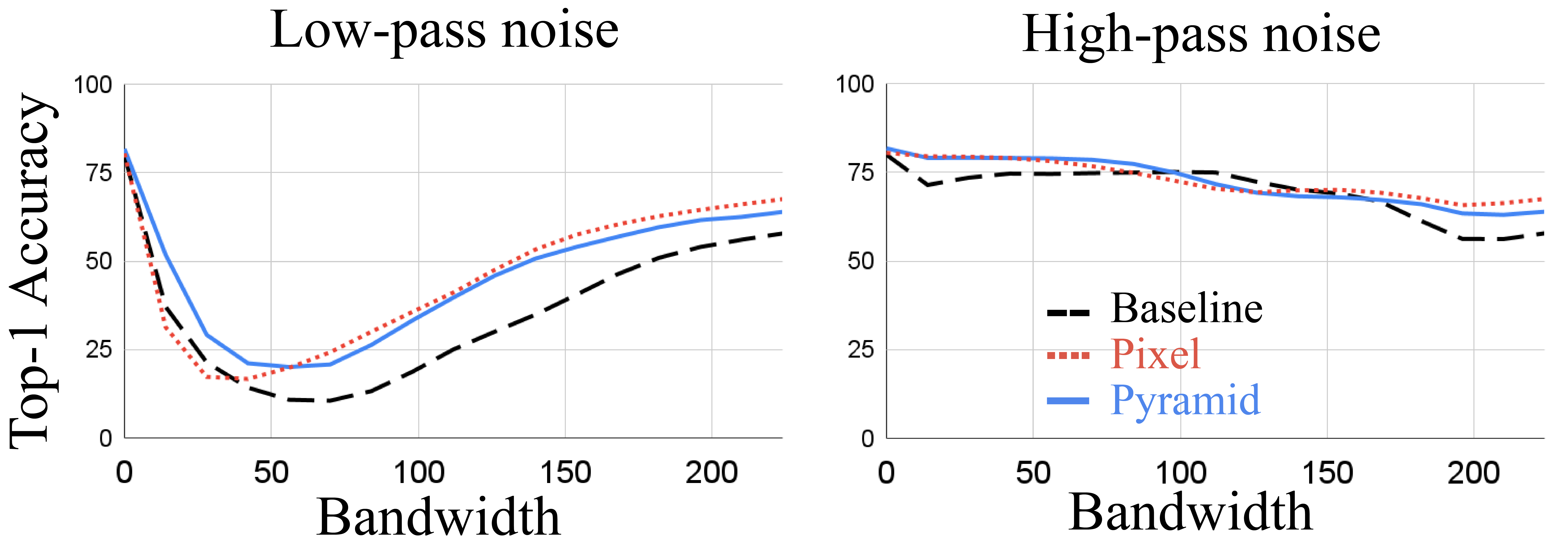
Inspired by [62], we analyze the pyramid adversarial training from a frequency perspective. For this analysis, all visualizations and graphs are averaged over the entire ImageNet validation set. Figure 6 shows a Fourier heat map of random and adversarial versions of the pixel and pyramid attacks. While random pixel noise is evenly concentrated over all frequencies, adversarial pixel attack tends to concentrate in the lower frequencies. Random pyramid shows a bias towards low frequency as well, a trend which is amplified in the adversarial pyramid. To further explore this, we replicate an analysis from [62], where low-pass- and high-pass-filtered random noise is added to test data to perturb a classifier. Figure 7 gives the result for our baseline, pixel, and pyramid adversarially trained models. While pixel and pyramid models are generally more robust than the baseline, the pyramid model is more robust than the pixel model to low-frequency perturbations.

Limitations

The cost of our technique is increased training time. A $k$ -step PGD attack requires $k$ forward and backward passes for each step of training. Note that this limitation holds for any adversarial training and the inference time is the same. Without adversarial training, more training time does not improve the baseline ViT-B/16.

5 Conclusion

We have introduced pyramid adversarial training, a simple and effective data augmentation technique that substantially improves the performance of ViT and MLP-Mixer architectures on in-distribution and a number of out-of-distribution ImageNet datasets.

References

[1] Anish Athalye, Nicholas Carlini, and David Wagner. Obfuscated gradients give a false sense of security: Circumventing defenses to adversarial examples. In International Conference on Machine Learning (ICML), pages 274–283. PMLR, 2018.
[2] Hangbo Bao, Li Dong, Songhao Piao, and Furu Wei. BEit: BERT pre-training of image transformers. In International Conference on Learning Representations (ICLR), 2022.
[3] Andrei Barbu, David Mayo, Julian Alverio, William Luo, Christopher Wang, Dan Gutfreund, Josh Tenenbaum, and Boris Katz. Objectnet: A large-scale bias-controlled dataset for pushing the limits of object recognition models. In Advances in Neural Information Processing Systems (NeurIPS), volume 32. Curran Associates, Inc., 2019.
[4] Lucas Beyer, Olivier J. Henaff, Alexander Kolesnikov, Xiaohua Zhai, and Aaron van den Oord. Are we done with imagenet? 2020.
[5] James Bradbury, Roy Frostig, Peter Hawkins, Matthew James Johnson, Chris Leary, Dougal Maclaurin, George Necula, Adam Paszke, Jake VanderPlas, Skye Wanderman-Milne, and Qiao Zhang. Jax: composable transformations of python+numpy programs. 2018.
[6] Nicholas Carlini and David Wagner. Towards evaluating the robustness of neural networks. In 2017 IEEE symposium on security and privacy (SP), pages 39–57. IEEE, 2017.
[7] Yair Carmon, Aditi Raghunathan, Ludwig Schmidt, John C Duchi, and Percy S Liang. Unlabeled data improves adversarial robustness. In Advances in Neural Information Processing Systems (NeurIPS), volume 32, 2019.
[8] Yong Cheng, Lu Jiang, and Wolfgang Macherey. Robust neural machine translation with doubly adversarial inputs. 2019.
[9] Yong Cheng, Lu Jiang, Wolfgang Macherey, and Jacob Eisenstein. Advaug: Robust adversarial augmentation for neural machine translation. 2020.
[10] Ekin Dogus Cubuk, Barret Zoph, Jon Shlens, and Quoc Le. Randaugment: Practical automated data augmentation with a reduced search space. In H. Larochelle, M. Ranzato, R. Hadsell, M. F. Balcan, and H. Lin, editors, Advances in Neural Information Processing Systems (NeurIPS), volume 33, pages 18613–18624. Curran Associates, Inc., 2020.
[11] Stephane d’Ascoli, Hugo Touvron, Matthew L Leavitt, Ari S Morcos, Giulio Biroli, and Levent Sagun. Convit: Improving vision transformers with soft convolutional inductive biases. In International Conference on Machine Learning (ICML), pages 2286–2296. PMLR, 2021.
[12] Mostafa Dehghani, Alexey Gritsenko, Anurag Arnab, Matthias Minderer, and Yi Tay. Scenic: A jax library for computer vision research and beyond. 2021.
[13] Jia Deng, Wei Dong, Richard Socher, Li-Jia Li, Kai Li, and Li Fei-Fei. Imagenet: A large-scale hierarchical image database. In 2009 IEEE conference on computer vision and pattern recognition, pages 248–255. Ieee, 2009.
[14] Terrance Devries and Graham W. Taylor. Improved regularization of convolutional neural networks with cutout. volume abs/1708.04552, 2017.
[15] Alexey Dosovitskiy, Lucas Beyer, Alexander Kolesnikov, Dirk Weissenborn, Xiaohua Zhai, Thomas Unterthiner, Mostafa Dehghani, Matthias Minderer, Georg Heigold, Sylvain Gelly, Jakob Uszkoreit, and Neil Houlsby. An image is worth 16x16 words: Transformers for image recognition at scale. In International Conference on Learning Representations (ICLR), 2021.
[16] Robert Geirhos, Patricia Rubisch, Claudio Michaelis, Matthias Bethge, Felix A Wichmann, and Wieland Brendel. Imagenet-trained CNNs are biased towards texture; increasing shape bias improves accuracy and robustness. In International Conference on Learning Representations (ICLR), 2019.
[17] Ian Goodfellow, Jonathon Shlens, and Christian Szegedy. Explaining and harnessing adversarial examples. In International Conference on Learning Representations (ICLR), 2015.
[18] Kaiming He, Xiangyu Zhang, Shaoqing Ren, and Jian Sun. Deep residual learning for image recognition. In Proceedings of the IEEE/CVF Conference on Computer Vision and Pattern Recognition (CVPR), pages 770–778, 2016.
[19] Dan Hendrycks, Steven Basart, Norman Mu, Saurav Kadavath, Frank Wang, Evan Dorundo, Rahul Desai, Tyler Zhu, Samyak Parajuli, Mike Guo, Dawn Song, Jacob Steinhardt, and Justin Gilmer. The many faces of robustness: A critical analysis of out-of-distribution generalization. 2021.
[20] Dan Hendrycks and Thomas Dietterich. Benchmarking neural network robustness to common corruptions and perturbations. In International Conference on Learning Representations (ICLR), 2019.
[21] Dan Hendrycks, Norman Mu, Ekin D Cubuk, Barret Zoph, Justin Gilmer, and Balaji Lakshminarayanan. Augmix: A simple data processing method to improve robustness and uncertainty. 2019.
[22] Dan Hendrycks, Kevin Zhao, Steven Basart, Jacob Steinhardt, and Dawn Song. Natural adversarial examples. 2021.
[23] Gao Huang, Yu Sun, Zhuang Liu, Daniel Sedra, and Kilian Q Weinberger. Deep networks with stochastic depth. In European conference on computer vision, pages 646–661. Springer, 2016.
[24] Sergey Ioffe and Christian Szegedy. Batch normalization: Accelerating deep network training by reducing internal covariate shift. In International Conference on Machine Learning (ICML), pages 448–456. PMLR, 2015.
[25] Insoo Kim, Seungju Han, Ji-won Baek, Seong-Jin Park, Jae-Joon Han, and Jinwoo Shin. Quality-agnostic image recognition via invertible decoder. In Proceedings of the IEEE/CVF Conference on Computer Vision and Pattern Recognition (CVPR), pages 12257–12266, June 2021.
[26] Diederik P. Kingma and Jimmy Ba. Adam: A method for stochastic optimization. In Yoshua Bengio and Yann LeCun, editors, International Conference on Learning Representations (ICLR), 2015.
[27] Alex Krizhevsky. Learning multiple layers of features from tiny images. Technical report, University of Toronto, 2009.
[28] Alexey Kurakin, Ian Goodfellow, and Samy Bengio. Adversarial machine learning at scale. 2016.
[29] Alexey Kurakin, Ian Goodfellow, and Samy Bengio. Adversarial machine learning at scale. 2016.
[30] Brenden M Lake, Tomer D Ullman, Joshua B Tenenbaum, and Samuel J Gershman. Building machines that learn and think like people. volume 40. Cambridge University Press, 2017.
[31] Shiyu Liang, Yixuan Li, and R. Srikant. Enhancing the reliability of out-of-distribution image detection in neural networks. In International Conference on Learning Representations (ICLR). OpenReview.net, 2018.
[32] Ze Liu, Yutong Lin, Yue Cao, Han Hu, Yixuan Wei, Zheng Zhang, Stephen Lin, and Baining Guo. Swin transformer: Hierarchical vision transformer using shifted windows. In Proceedings of the IEEE/CVF International Conference on Computer Vision (ICCV), pages 10012–10022, October 2021.
[33] Raphael Gontijo Lopes, Dong Yin, Ben Poole, Justin Gilmer, and Ekin Dogus Cubuk. Improving robustness without sacrificing accuracy with patch gaussian augmentation. volume abs/1906.02611, 2019.
[34] Ilya Loshchilov and Frank Hutter. SGDR: stochastic gradient descent with warm restarts. In International Conference on Learning Representations (ICLR). OpenReview.net, 2017.
[35] Aleksander Madry, Aleksandar Makelov, Ludwig Schmidt, Dimitris Tsipras, and Adrian Vladu. Towards deep learning models resistant to adversarial attacks. In International Conference on Learning Representations (ICLR). OpenReview.net, 2018.
[36] Kaleel Mahmood, Rigel Mahmood, and Marten van Dijk. On the robustness of vision transformers to adversarial examples. In Proceedings of the IEEE/CVF International Conference on Computer Vision (ICCV), pages 7838–7847, October 2021.
[37] Chengzhi Mao, Lu Jiang, Mostafa Dehghani, Carl Vondrick, Rahul Sukthankar, and Irfan Essa. Discrete representations strengthen vision transformer robustness. In International Conference on Learning Representations (ICLR), 2022.
[38] Xiaofeng Mao, Gege Qi, Yuefeng Chen, Xiaodan Li, Ranjie Duan, Shaokai Ye, Yuan He, and Hui Xue. Towards robust vision transformer. volume abs/2105.07926, 2021.
[39] Takeru Miyato, Shin-ichi Maeda, Masanori Koyama, and Shin Ishii. Virtual adversarial training: a regularization method for supervised and semi-supervised learning. volume 41, pages 1979–1993. IEEE, 2018.
[40] Seyed-Mohsen Moosavi-Dezfooli, Alhussein Fawzi, Jonathan Uesato, and Pascal Frossard. Robustness via curvature regularization, and vice versa. In Proceedings of the IEEE/CVF Conference on Computer Vision and Pattern Recognition (CVPR), pages 9078–9086, 2019.
[41] Muhammad Muzammal Naseer, Kanchana Ranasinghe, Salman H Khan, Munawar Hayat, Fahad Shahbaz Khan, and Ming-Hsuan Yang. Intriguing properties of vision transformers. In Advances in Neural Information Processing Systems (NeurIPS), volume 34, 2021.
[42] Yuval Netzer, Tao Wang, Adam Coates, Alessandro Bissacco, Bo Wu, and Andrew Y Ng. Reading digits in natural images with unsupervised feature learning. In Advances in Neural Information Processing Systems (NeurIPS), 2011.
[43] Nicolas Papernot, Patrick McDaniel, Xi Wu, Somesh Jha, and Ananthram Swami. Distillation as a defense to adversarial perturbations against deep neural networks. In 2016 IEEE symposium on security and privacy (SP), pages 582–597. IEEE, 2016.
[44] Chongli Qin, James Martens, Sven Gowal, Dilip Krishnan, Krishnamurthy Dvijotham, Alhussein Fawzi, Soham De, Robert Stanforth, and Pushmeet Kohli. Adversarial robustness through local linearization. In Advances in Neural Information Processing Systems (NeurIPS), volume 32, 2019.
[45] Aditi Raghunathan, Sang Michael Xie, Fanny Yang, John C. Duchi, and Percy Liang. Understanding and mitigating the tradeoff between robustness and accuracy. volume abs/2002.10716, 2020.
[46] René Ranftl, Alexey Bochkovskiy, and Vladlen Koltun. Vision transformers for dense prediction. In Proceedings of the IEEE/CVF International Conference on Computer Vision (ICCV), pages 12179–12188, October 2021.
[47] Benjamin Recht, Rebecca Roelofs, Ludwig Schmidt, and Vaishaal Shankar. Do imagenet classifiers generalize to imagenet? In International Conference on Machine Learning (ICML), pages 5389–5400. PMLR, 2019.
[48] Olga Russakovsky, Jia Deng, Hao Su, Jonathan Krause, Sanjeev Satheesh, Sean Ma, Zhiheng Huang, Andrej Karpathy, Aditya Khosla, Michael Bernstein, Alexander C. Berg, and Li Fei-Fei. ImageNet Large Scale Visual Recognition Challenge. volume 115, pages 211–252, 2015.
[49] Rulin Shao, Zhouxing Shi, Jinfeng Yi, Pin-Yu Chen, and Cho-Jui Hsieh. On the adversarial robustness of visual transformers. volume abs/2103.15670, 2021.
[50] Nitish Srivastava, Geoffrey Hinton, Alex Krizhevsky, Ilya Sutskever, and Ruslan Salakhutdinov. Dropout: A simple way to prevent neural networks from overfitting. volume 15, pages 1929–1958, 2014.
[51] Andreas Steiner, Alexander Kolesnikov, Xiaohua Zhai, Ross Wightman, Jakob Uszkoreit, and Lucas Beyer. How to train your vit? data, augmentation, and regularization in vision transformers. volume abs/2106.10270, 2021.
[52] Christian Szegedy, Wojciech Zaremba, Ilya Sutskever, Joan Bruna, Dumitru Erhan, Ian Goodfellow, and Rob Fergus. Intriguing properties of neural networks. 2013.
[53] Mingxing Tan and Quoc Le. Efficientnet: Rethinking model scaling for convolutional neural networks. In International Conference on Machine Learning (ICML), pages 6105–6114. PMLR, 2019.
[54] Ilya O Tolstikhin, Neil Houlsby, Alexander Kolesnikov, Lucas Beyer, Xiaohua Zhai, Thomas Unterthiner, Jessica Yung, Andreas Steiner, Daniel Keysers, Jakob Uszkoreit, et al. Mlp-mixer: An all-mlp architecture for vision. In Advances in Neural Information Processing Systems (NeurIPS), volume 34, 2021.
[55] Hugo Touvron, Matthieu Cord, Matthijs Douze, Francisco Massa, Alexandre Sablayrolles, and Hervé Jégou. Training data-efficient image transformers & distillation through attention. In International Conference on Machine Learning (ICML), pages 10347–10357. PMLR, 2021.
[56] Dimitris Tsipras, Shibani Santurkar, Logan Engstrom, Alexander Turner, and Aleksander Madry. Robustness may be at odds with accuracy, 2019.
[57] Abraham Wald. Statistical decision functions which minimize the maximum risk. pages 265–280. JSTOR, 1945.
[58] Haohan Wang, Songwei Ge, Zachary Lipton, and Eric P Xing. Learning robust global representations by penalizing local predictive power. In Advances in Neural Information Processing Systems (NeurIPS), pages 10506–10518, 2019.
[59] Haotao Wang, Chaowei Xiao, Jean Kossaifi, Zhiding Yu, Anima Anandkumar, and Zhangyang Wang. Augmax: Adversarial composition of random augmentations for robust training. In Advances in Neural Information Processing Systems (NeurIPS), volume 34, 2021.
[60] Chaowei Xiao, Jun-Yan Zhu, Bo Li, Warren He, Mingyan Liu, and Dawn Song. Spatially transformed adversarial examples. 2018.
[61] Cihang Xie, Mingxing Tan, Boqing Gong, Jiang Wang, Alan L Yuille, and Quoc V Le. Adversarial examples improve image recognition. In Proceedings of the IEEE/CVF International Conference on Computer Vision (ICCV), pages 819–828, 2020.
[62] Dong Yin, Raphael Gontijo Lopes, Jon Shlens, Ekin Dogus Cubuk, and Justin Gilmer. A fourier perspective on model robustness in computer vision. In Advances in Neural Information Processing Systems (NeurIPS), volume 32, 2019.
[63] Sangdoo Yun, Dongyoon Han, Seong Joon Oh, Sanghyuk Chun, Junsuk Choe, and Youngjoon Yoo. Cutmix: Regularization strategy to train strong classifiers with localizable features. In Proceedings of the IEEE/CVF International Conference on Computer Vision (ICCV), pages 6023–6032, 2019.
[64] Hongyi Zhang, Moustapha Cisse, Yann N Dauphin, and David Lopez-Paz. mixup: Beyond empirical risk minimization. 2017.
[65] Hongyang Zhang, Yaodong Yu, Jiantao Jiao, Eric Xing, Laurent El Ghaoui, and Michael Jordan. Theoretically principled trade-off between robustness and accuracy. In Kamalika Chaudhuri and Ruslan Salakhutdinov, editors, Proceedings of the 36th International Conference on Machine Learning, volume 97 of Proceedings of Machine Learning Research, pages 7472–7482. PMLR, 09–15 Jun 2019.
[66] Juntang Zhuang, Tommy Tang, Yifan Ding, Sekhar C Tatikonda, Nicha Dvornek, Xenophon Papademetris, and James Duncan. Adabelief optimizer: Adapting stepsizes by the belief in observed gradients. In Advances in Neural Information Processing Systems (NeurIPS), volume 33, pages 18795–18806, 2020.

Thanks for viewing the supplementary material, in which we provide a detailed explanation of the pyramid structure in Section A, detailed experiments for different backbones in Section B, more ablation study in Section C, additional analysis in Section D, visualizations in Section E, and finally a discussion on the effect of optimizers in Section F.

Appendix A Pyramid Attack Details

In this section, we provide a conceptual description and pseudocode for the pyramid attack.

Description

Scale $s$ determines the size of the patch that an individual perturbation parameter will be applied to; e.g. for $s\!=\!16$ , we learn and add a single adv parameter to each non-overlapping patch of size 16x16. The application is equivalent to a nearest neighbor resize on the 14x14 adv tensor to the image size of 224x224 and then addition. The scales $s$ and multipliers $m_{s}$ used by PyramidAT are hyperparameters.

Code

We provide a minimal implementation of our technique in Fig. 8.

⬇

import jax

import jax.numpy as jnp

H=224,lr=1/255, M=[20,10,1], S=[32,16,1], BOUNDS=[0, 1], n_steps=5

def get_attacked_image(model, loss_fn, image):

def get_perturbed_image(delta):

return image + sum(

M[i]*jax.image.resize(delta[i], (H,H,3), ’nearest’)

for i in delta)

def get_perturbed_loss(delta):

return loss_fn(model(get_perturbed_image(delta)))

delta = {i: jnp.zeros((H/s, H/s, 3)) for (i,s) in enumerate(S)}

for _ in range(n_steps):

delta_grad = jax.grad(get_perturbed_loss)(delta)

delta = {i: delta[i]+lr*jnp.sign(delta_grad[i]) for i in delta}

perturbed_image = get_perturbed_image(delta)

return jnp.clip(perturbed_image, BOUNDS[0], BOUNDS[1])

Figure 8: Implementation of our technique in JAX.

Appendix B Discussing Backbones

B.1 ResNets

Table 10 shows results for multiple variants of ResNet[18]: ResNet-50, ResNet-101, and ResNet-200. As the capacity of the network increases, we observe larger gains from both PixelAT and PyramidAT. PyramidAT performs the best on all evaluation sets.

For these runs, we follow the training protocol and network details set up in [61]. We use the proposed split BN and standard ResNet training: 90 epochs, cosine learning rate at 0.1 with linear warmup for 7 epochs, minimal augmentations (left right flip and Inception crop). For network optimization, we use SGD with momentum and for the adversarial steps, we use SGD.

			Out of Distribution Robustness Test
Method	ImageNet	Real	A	C $\downarrow$	ObjectNet	V2	Rendition	Sketch	Stylized
ResNet-50	76.70	83.11	4.49	74.90	26.47	64.31	36.24	23.44	6.41
+PixelAT	77.37	84.11	6.03	66.88	27.80	65.59	41.75	27.04	8.13
+PyramidAT	77.48	84.22	6.24	66.77	27.91	65.96	43.32	28.55	8.83
ResNet-101	78.44	84.29	6.16	69.75	29.31	66.54	38.74	26.15	7.19
+PixelAT	79.57	85.73	9.55	59.92	31.00	67.95	44.63	29.83	10.23
+PyramidAT	79.69	85.82	9.96	59.15	31.57	68.12	46.50	31.74	10.94
ResNet-200	79.47	85.25	8.65	65.58	31.86	67.36	40.55	28.21	7.81
+PixelAT	80.51	86.34	12.93	56.99	33.84	69.73	46.32	32.74	9.14
+PyramidAT	80.92	86.59	14.17	55.72	34.04	70.08	48.05	34.54	11.48

Table 10: For all variants of ResNet, PyramidAT leads to improvements. Note that this is with the standard training of ResNet.

B.2 ViT Tiny/16

ViT Ti/16 has the same overall structure and design as ViT B/16 (the primary model used in our main paper) but is significantly smaller, at 5.8 million parameters (as opposed to the 86 million parameters of B/16). More specifically, Ti/16 has a width of 192 (instead of 768), MLP size of 768 (instead of 3072), and 3 heads (instead of 12). In total, this decrease in parameters and model size leads to a substantial decrease in capacity. We experiment with ViT Ti/16 primarily in order to understand the impact of this decreased capacity on our adversarial training methods.

We start with an exploration of the impact of the random augmentation’s strength on the overall performance of the model. Table 11 shows the performance of Ti/16 models with different RandAugment parameters (the two parameters are in order the number of transforms applied and the magnitude of the transforms); this table suggests that the network’s lower capacity benefits from weaker random augmentation. Specifically, the best RandAugment parameters for the majority of the evaluation datasets is (1,0.8), which is considerably lower than the RandAugment parameters tuned for B/16 (2, 15).

			Out of Distribution Robustness Test
Method	ImageNet	Real	A	C $\downarrow$	ObjectNet	V2	Rendition	Sketch	Stylized
RA=(2,10)	61.07	68.77	3.95	85.84	12.88	48.50	21.95	11.21	4.84
RA=(2,5)	64.62	72.57	4.59	80.79	15.44	52.37	25.68	14.48	8.36
RA=(1,10)	63.64	71.26	4.64	83.04	14.53	51.37	23.67	13.14	7.27
RA=(1,5)	64.96	72.54	4.80	81.32	14.94	52.05	25.03	13.69	8.98
RA=(1,3)	64.88	72.66	4.80	79.04	15.61	52.59	25.43	13.54	8.13
RA=(1,0.8)	65.33	73.19	4.79	77.08	16.16	53.03	25.98	14.15	8.98
RA=(1,0.4)	64.27	72.17	4.69	78.10	15.46	52.18	24.99	13.47	8.59
RA=(1,0.1)	63.58	71.41	4.80	79.23	15.39	51.43	23.66	12.54	8.36

Table 11: ViT Ti/16 baseline training with different random augmentations. In this table, RA denotes the two RandAugment parameters: number of applied transforms, and mangitude of transforms. Note that weaker augmentation tends to perform better.

In Table 12 and 13, we pick several of the better performing RandAugment parameters and then show results from adversarial training with steps of 1 and 3, respectively.

Table 12 shows that the performance of adversarial training depends heavily on both the random augmentation and the type of attack. Note, RAm refers to the RandAugment mangitude parameter. As shown by RAm=0.1, pixel attacks can improve performance for in-distribution evaluation datasets when the random augmentation strength is low. However, at higher random augmentation, RAm=0.4 and RAm=0.8, PixelAT leads to the commonly observed trade-off between clean performance and adversarial robustness. In contrast, pyramid tends to improve performance across the board regardless of the starting augmentation (for all RAm of 0.1, 0.4, and 0.8). Interestingly, PixelAT exhibits better robustness properties (out-of-distribution performance) than PyramidAT for Ti/16. We hypothesize that the limited capacity can be “spent” on either in-distribution or out-of-distribution representations and that pyramid tends to bias the network towards in-distribution as opposed to pixel which has a bias towards out-of-distribution.

			Out of Distribution Robustness Test
Method	ImageNet	Real	A	C $\downarrow$	ObjectNet	V2	Rendition	Sketch	Stylized
Ti/16 RAm=0.1	63.58	71.41	4.80	79.23	15.39	51.43	23.66	12.54	8.36
+PixelAT steps=1	64.66	72.75	4.39	74.54	14.61	52.05	32.52	17.65	14.77
+PyramidAT steps=1	65.49	73.53	5.16	74.30	16.15	53.08	29.18	16.55	12.58
Ti/16 RAm=0.4	64.27	72.17	4.69	78.10	15.46	52.18	24.99	13.47	8.59
+PixelAT steps=1	62.78	70.53	4.05	77.67	13.89	50.37	29.75	16.35	11.80
+PyramidAT steps=1	65.61	73.68	4.80	74.72	15.97	52.88	28.89	16.14	11.95
Ti/16 RAm=0.8	65.33	73.19	4.79	77.08	16.16	53.03	25.98	14.15	8.98
+PixelAT steps=1	63.49	71.64	3.80	75.68	13.79	51.13	31.80	17.65	13.91
+PyramidAT steps=1	65.67	73.73	4.84	75.25	15.71	53.43	29.08	16.41	12.97

Table 12: ViT Ti/16 adversarial training experiments with steps=1. RAm gives the RandAugment magnitude parameter; all experiments have RandAugment number of transforms equal to 1. Pixel’s performance on 0.4 and 0.8 is consistent with earlier work that suggests that adversarial training causes a trade-off between in distribution and out of distribution datasets. However, we show that a low random augmentation starting point can break this trade-off and lead to gains. Pyramid tends to outperform pixel on in-distribution performance for all random augmentations. However, pixel performs well for out-of-distribution datasets.

Table 13 shows that the strength of the adversarial attack also matters substantially to the overall performance of the model. Both attacks, pixel and pyramid, with 3 steps tend to degrade the model’s performance on in-distribution evaluation datasets. Adversarial training still provides some benefits for out-of-distribution, with pyramid performing the best in terms of robustness. We hypothesize that pyramid outperforms pixel in the steps=3 runs because pyramid is a weaker out-of-distribution augmentation and pixel at 3 steps has over-regularized the network, leading to decreased performance. Note that pyramid at steps=3 produces the best out-of-distribution performance out of any Ti/16 runs including strong random augmentation and PixelAT at steps=1.

			Out of Distribution Robustness Test
Method	ImageNet	Real	A	C $\downarrow$	ObjectNet	V2	Rendition	Sketch	Stylized
Ti/16 RAm=0.1	63.58	71.41	4.80	79.23	15.39	51.43	23.66	12.54	8.36
+PixelAT steps=3	59.91	67.77	3.39	81.44	12.04	47.28	28.52	14.78	11.02
+PyramidAT steps=3	62.71	71.08	4.08	74.49	14.72	50.25	35.05	20.67	18.67
Ti/16 RAm=0.8	65.33	73.19	4.79	77.08	16.16	53.03	25.98	14.15	8.98
+PixelAT steps=3	60.10	67.88	3.36	80.48	11.90	47.78	29.83	15.21	13.44
+PyramidAT steps=3	62.92	71.11	4.05	74.70	14.76	50.77	34.74	20.35	18.13

Table 13: ViT Ti/16 adversarial training experiments with steps=3. RAm gives the RandAugment magnitude parameter; all experiments have RandAugment number of transforms equal to 1. All techniques degrade from the baseline suggesting that 3 adversarial steps produces augmentation that is too strong for Ti’s capacity.

B.3 MLP-Mixer

As shown in the main paper, we observe gains across the board for MLP-Mixer with PyramidAT. Here, we show that the gain is robust to a change in the LR schedule and that the gain is, again, affected by the starting augmentation.

Table 14 shows baseline and adversarially trained models for two different training schedules of MLP-Mixer, one with the default LR schedule of 10k warm-up steps and then linear decay to an end learning rate (LR) of $1e-5$ and another with a more aggressive end learning rate of $1e-7$ . We show that this change in LR schedule does not affect the gains from adversarial training.

			Out of Distribution Robustness Test
Method	ImageNet	Real	A	C $\downarrow$	ObjectNet	V2	Rendition	Sketch	Stylized
MLP-Mixer [54] end LR=1e-5 (default)	78.27	83.64	10.84	58.50	25.90	64.97	38.51	29.00	10.08
+PixelAT	77.17	82.99	9.93	57.68	24.75	64.03	44.43	33.68	15.31
+PyramidAT	79.29	84.78	12.97	52.88	28.60	66.56	45.34	34.79	14.77
MLP-Mixer [54] end LR=1e-7	75.92	81.28	9.45	64.29	22.13	62.17	33.70	25.15	7.27
+PixelAT	74.96	80.81	7.81	61.85	20.87	60.94	39.82	28.59	12.27
+PyramidAT	77.98	83.60	11.17	56.19	25.59	64.92	41.65	31.99	12.66

Table 14: MLP-Mixer ablations with different training. The pyramid gains are preserved even with different training schedules.

Table 15 shows that, similar to ViT Ti/16, the gains are improved when the random augmentation is weakened. However, in this case, the gain is not enough to overcome the drop in performance from using the weaker augmentation.

			Out of Distribution Robustness Test
Method	ImageNet	Real	A	C $\downarrow$	ObjectNet	V2	Rendition	Sketch	Stylized
MLP-Mixer [54] end LR=1e-7, RA=(2,15)	75.92	81.28	9.45	64.29	22.13	62.17	33.70	25.15	7.27
+PixelAT	74.96	80.81	7.81	61.85	20.87	60.94	39.82	28.59	12.27
+PyramidAT	77.98	83.60	11.17	56.19	25.59	64.92	41.65	31.99	12.66
MLP-Mixer [54] end LR=1e-7, RA=(2,9)	73.56	79.01	7.79	67.18	18.09	60.30	31.47	22.80	7.58
+PixelAT	72.44	78.27	7.80	63.38	16.96	58.40	37.18	25.78	12.27
+PyramidAT	76.19	81.47	10.61	57.71	21.86	63.03	39.52	29.40	14.37

Table 15: MLP-Mixer ablations with random augmentation magnitude. Weaker random augmentations lead to larger gains from the adversarial training but with these parameters do not lead to better overall performance than the strong random augmentation plus adversarial training. Note that for both the starting point and weaker random augmentation, the gain from pyramid is substantial compared to the gain from pixel.

Appendix C Additional Ablations

C.1 Dropout

One of the key findings of this paper is the importance of “matched” Dropout[50] and stochastic depth[23]. Here we describe numerous ablations on these Dropout terms and list several detailed findings including:

•

Matching the Dropout and stochastic depth matters significantly for balanced clean performance and robustness.
•

Running without Dropout in the adversarial training branch can improve robustness even more.
•

Dropout matters more than Stochastic Depth

Note that in the tables below, we use the term “dropparams” to refer to a tuple of the Dropout probability and stochastic depth probability. Clean dropparams (abbreviated as c_dp) refer to the dropparams used for the clean training branch; adversarial dropparams (abbreviated as a_dp) refer to the dropparams used for the adversarial training branch; and matched dropparams (abbreviated as m_dp) refer to dropparams used for both clean and adversarial branches. So $\textrm{c\_dp}=(10,0)$ means that the clean training branch had a 10% probability of Dropout but a 0% probability of stochastic depth.

Table 16 explores different possible values for adversarial dropparams. In general, lower values of Dropout and stochastic depth in the adversarial branch improve out-of-distribution performance while hurting in-distribution performance; however, the opposite is not true: higher levels of Dropout and stochastic depth in the adversarial branch do not improve in-distribution performance. In-distribution performance seems to peak when the params for the adversarial and clean branches match.

			Out of Distribution Robustness Test
Method	ImageNet	Real	A	C $\downarrow$	ObjectNet	V2	Rendition	Sketch	Stylized
Baseline $\textrm{c\_dp}=(10,10)$	79.92	85.14	17.48	52.46	29.30	67.49	38.24	29.08	11.02
PixelAT $\textrm{a\_dp}=(0,0)$	79.13	84.75	14.37	52.73	29.01	66.94	49.94	37.03	22.34
PixelAT $\textrm{a\_dp}=(5,5)$	78.41	84.39	14.00	54.50	28.04	66.30	49.29	36.84	21.80
PixelAT $\textrm{a\_dp}=(10,10)$	80.42	85.78	19.15	47.68	30.11	68.78	45.39	34.40	18.28
PixelAT $\textrm{a\_dp}=(20,20)$	81.00	86.16	21.43	46.07	30.85	69.60	46.00	34.73	18.36
PixelAT $\textrm{a\_dp}=(30,30)$	76.53	82.56	16.20	66.09	24.22	64.40	42.93	34.89	15.00
Baseline $\textrm{c\_dp}=(10,10)$	79.92	85.14	17.48	52.46	29.30	67.49	38.24	29.08	11.02
PyramidAT $\textrm{a\_dp}=(0,0)$	79.31	85.13	13.95	55.09	29.98	67.43	53.69	41.07	23.44
PyramidAT $\textrm{a\_dp}=(5,5)$	79.13	84.90	13.43	54.08	28.99	67.50	52.39	40.23	24.84
PyramidAT $\textrm{a\_dp}=(10,10)$	81.71	86.82	22.99	44.99	32.92	70.82	47.66	36.77	19.14
PyramidAT $\textrm{a\_dp}=(20,20)$	81.67	86.76	23.33	45.19	32.74	70.58	48.15	38.01	17.50
PyramidAT $\textrm{a\_dp}=(30,30)$	74.26	80.57	11.55	69.85	22.87	61.46	41.59	29.89	17.66

Table 16: Ablation on the values of Dropout and stochastic depth for adversarial training branch. All c_dp are kept constant at

(10,10)

in the adversarial section.

Table 17 explores different possible values for matched dropparams. In general, the dropparams determined by RegViT[51] seem to be roughly optimal for both the baselines and the adversarially trained models, with some variation for some datasets.

			Out of Distribution Robustness Test
Method	ImageNet	Real	A	C $\downarrow$	ObjectNet	V2	Rendition	Sketch	Stylized
Baseline $\textrm{c\_dp}=(0,0)$	75.69	80.92	12.68	61.78	23.65	62.49	34.23	24.38	7.73
Baseline $\textrm{c\_dp}=(5,5)$	79.05	84.19	16.52	54.32	28.27	66.40	37.38	28.08	9.53
Baseline $\textrm{c\_dp}=(10,10)$	79.92	85.14	17.48	52.46	29.30	67.49	38.24	29.08	11.02
Baseline $\textrm{c\_dp}=(15,15)$	79.35	84.74	17.71	52.96	29.11	67.47	39.13	28.67	11.41
Baseline $\textrm{c\_dp}=(20,20)$	78.40	84.24	16.16	54.93	27.80	66.07	37.85	27.77	9.84
PixelAT $\textrm{m\_dp}=(0,0)$	79.13	84.20	19.71	49.68	29.77	67.02	43.34	32.14	15.23
PixelAT $\textrm{m\_dp}=(5,5)$	80.82	85.59	22.12	46.15	31.27	68.99	44.86	33.31	16.95
PixelAT $\textrm{m\_dp}=(10,10)$	80.42	85.78	19.15	47.68	30.11	68.78	45.39	34.40	18.28
PixelAT $\textrm{m\_dp}=(15,15)$	79.03	84.88	15.16	50.67	27.72	66.53	46.43	34.21	21.95
PixelAT $\textrm{m\_dp}=(20,20)$	77.89	84.12	13.99	52.20	26.28	66.06	45.21	32.75	21.95
PyramidAT $\textrm{m\_dp}=(0,0)$	79.54	84.66	18.91	50.02	30.10	67.44	44.43	33.46	13.67
PyramidAT $\textrm{m\_dp}=(5,5)$	81.80	86.59	23.47	45.52	32.76	70.36	46.62	36.50	17.27
PyramidAT $\textrm{m\_dp}=(10,10)$	81.71	86.82	22.99	44.99	32.92	70.82	47.66	36.77	19.14
PyramidAT $\textrm{m\_dp}=(15,15)$	80.95	86.49	21.33	46.18	31.62	69.70	47.21	36.83	18.91
PyramidAT $\textrm{m\_dp}=(20,20)$	79.56	85.77	18.35	49.14	29.73	68.13	45.72	35.41	18.36

Table 17: Ablation on the values of Dropout and stochatic depth for matched attacks.

Table 18 explores if one of these parameters is more important than the others. To do so, we set clean dropparams to $(10,10)$ for the entire table (besides the included baselines) and only vary the adversarial dropparams. For both PixelAT and PyramidAT, the Dropout parameter seems to be more important for clean, in-distribution performance. Without Dropout, the top-1 of ImageNet drops $0.41$ for PixelAT and $0.92$ for PyramidAT. However, no Dropout does give a substantial boost to out-of-distribution performance, with Rendition gains of $11.59$ for PixelAT and $15.68$ for PyramidAT and Sketch gains of $7.49$ for PixelAT and $11.96$ for PyramidAT. Without stochastic depth, the adversarially trained models seem to perform roughly as well as with stochastic depth, exhibitly marginally more clean accuracy for PyramidAT than the model with both Dropout and stochastic depth. Our main takeaway is that Dropout seems to be the primary determinant in whether the gains are balanced between in-distribution and out-of-distribution or primarily focused on out-of-distribution. In fact, no Dropout PyramidAT performs so well on out-of-distribution that it sets new state-of-the-art numbers for Rendition and Sketch.

			Out of Distribution Robustness Test
Method	ImageNet	Real	A	C $\downarrow$	ObjectNet	V2	Rendition	Sketch	Stylized
Baseline $\textrm{c\_dp}=(0,0)$	75.69	80.92	12.68	61.78	23.65	62.49	34.23	24.38	7.73
Baseline $\textrm{c\_dp}=(10,10)$	79.92	85.14	17.48	52.46	29.30	67.49	38.24	29.08	11.02
PixelAT $\textrm{a\_dp}=(0,10)$	79.40	84.98	14.32	52.17	28.87	67.24	49.83	36.57	21.88
PixelAT $\textrm{a\_dp}=(10,0)$	79.51	85.12	15.65	49.38	29.45	67.50	47.32	34.64	21.17
PixelAT $\textrm{a\_dp}=(10,10)$	80.42	85.78	19.15	47.68	30.11	68.78	45.39	34.40	18.28
PyramidAT $\textrm{a\_dp}=(0,10)$	79.00	85.02	13.69	55.58	29.38	66.96	53.92	41.04	24.22
PyramidAT $\textrm{a\_dp}=(10,0)$	81.80	86.67	23.51	45.00	33.37	70.52	47.82	37.09	19.38
PyramidAT $\textrm{a\_dp}=(10,10)$	81.71	86.82	22.99	44.99	32.92	70.82	47.66	36.77	19.14

Table 18: Ablation on the values of Dropout and stochastic depth for unmatched attacks. For the adversarial techniques, clean dropparams will be the same as RegVit at (10, 10). For the adversarial training rows, either Dropout or stochastic depth will be 0 and the other will be the base value. This table explores whether one of these parameters is more important than the other. For both PixelAT and PyramidAT, Dropout appears to be more important in determining the balance between in-distribution and out-of-distribution performance. PyramidAT no Dropout is SOTA for Rendition and Sketch.

Table 19 explores parameter settings where the Dropout and stochastic depth are not equal. In general, there does not seem to be a consistent trend or recognizable pattern for the overall performance, though some patterns exist for specific attacks and evaluation datasets. For example, increasing stochastic depth probability for pixel attacks tend to improve Real, ImageNet-C, and ObjectNet performance.

			Out of Distribution Robustness Test
Method	ImageNet	Real	A	C $\downarrow$	ObjectNet	V2	Rendition	Sketch	Stylized
Baseline $\textrm{c\_dp}=(10,10)$	79.92	85.14	17.48	52.46	29.30	67.49	38.24	29.08	11.02
PixelAT $\textrm{a\_dp}=(0,10)$	79.40	84.98	14.32	52.17	28.87	67.24	49.83	36.57	21.88
PixelAT $\textrm{a\_dp}=(10,10)$	80.42	85.78	19.15	47.68	30.11	68.78	45.39	34.40	18.28
PixelAT $\textrm{a\_dp}=(20,10)$	74.58	80.74	13.07	69.14	23.93	61.82	42.64	33.54	17.42
PixelAT $\textrm{a\_dp}=(30,10)$	80.14	85.59	20.91	48.99	29.74	68.50	44.62	35.06	16.02
PixelAT $\textrm{a\_dp}=(10,0)$	79.51	85.12	15.65	49.38	29.45	67.50	47.32	34.64	21.17
PixelAT $\textrm{a\_dp}=(10,10)$	80.42	85.78	19.15	47.68	30.11	68.78	45.39	34.40	18.28
PixelAT $\textrm{a\_dp}=(10,20)$	81.14	86.22	21.37	45.91	31.53	69.75	46.24	35.14	19.45
PixelAT $\textrm{a\_dp}=(10,30)$	80.94	86.26	21.37	45.19	31.63	69.69	45.76	34.69	19.61
PyramidAT $\textrm{a\_dp}=(0,10)$	79.00	85.02	13.69	55.58	29.38	66.96	53.92	41.04	24.22
PyramidAT $\textrm{a\_dp}=(10,10)$	81.71	86.82	22.99	44.99	32.92	70.82	47.66	36.77	19.14
PyramidAT $\textrm{a\_dp}=(20,10)$	75.36	81.40	14.03	70.76	23.65	63.14	39.36	26.92	15.00
PyramidAT $\textrm{a\_dp}=(30,10)$	79.18	84.91	17.43	56.44	28.95	67.81	43.64	29.91	19.45
PyramidAT $\textrm{a\_dp}=(10,0)$	81.80	86.67	23.51	45.00	33.37	70.52	47.82	37.09	19.38
PyramidAT $\textrm{a\_dp}=(10,10)$	81.71	86.82	22.99	44.99	32.92	70.82	47.66	36.77	19.14
PyramidAT $\textrm{a\_dp}=(10,20)$	81.50	86.58	23.13	45.72	32.45	70.48	48.08	36.91	17.66
PyramidAT $\textrm{a\_dp}=(10,30)$	81.53	86.75	21.87	45.59	32.80	70.34	47.73	37.12	17.89

Table 19: Ablation on settings where the Dropout parameter and stochastic depth parameter are not equal for adversarial training branch. All c_dp are kept constant at

(10,10)

in the adversarial section.

Table 20 explores the effects of adversarial training with different dropparams without Dropout or stochastic depth in the main branch. In general, the lack of Dropout and stochastic depth in the clean branch has a substantial negative effect on the performance of the model and all of the resulting models under-perform their counterparts with non-zero clean dropparams. In this setting, adversarial training does provide substantial improvements for both in-distribution ( $+5.18$ for clean using PyramidAT) and out-of-distribution performances ( $+12.29$ for Rendition using PyramidAT and $+11.68$ for Sketch using PyramidAT), but not enough to offset the poor starting performance of the baseline model.

			Out of Distribution Robustness Test
Method	ImageNet	Real	A	C $\downarrow$	ObjectNet	V2	Rendition	Sketch	Stylized
Baseline $\textrm{c\_dp}=(0,0)$	75.69	80.92	12.68	61.78	23.65	62.49	34.23	24.38	7.73
PixelAT $\textrm{c\_dp}=(0,0)$ $\textrm{a\_dp}=(5,5)$	79.86	84.78	21.23	48.66	30.19	67.92	43.94	32.69	15.00
PixelAT $\textrm{c\_dp}=(0,0)$ $\textrm{a\_dp}=(10,10)$	79.82	84.81	21.32	47.82	30.84	67.99	43.25	32.24	14.92
PixelAT $\textrm{c\_dp}=(0,0)$ $\textrm{a\_dp}=(20,20)$	80.03	84.96	21.69	47.86	31.34	68.16	43.56	32.78	14.77
Baseline $\textrm{c\_dp}=(0,0)$	75.69	80.92	12.68	61.78	23.65	62.49	34.23	24.38	7.73
PyramidAT $\textrm{c\_dp}=(0,0)$ $\textrm{a\_dp}=(5,5)$	80.79	85.66	23.65	47.39	32.39	69.12	46.30	36.40	15.70
PyramidAT $\textrm{c\_dp}=(0,0)$ $\textrm{a\_dp}=(10,10)$	80.69	85.55	23.25	47.14	32.74	69.21	46.49	36.09	15.78
PyramidAT $\textrm{c\_dp}=(0,0)$ $\textrm{a\_dp}=(15,15)$	80.87	85.74	23.63	46.68	32.67	69.27	46.52	36.06	17.19

Table 20: Ablation on the values of Dropout and stochastic depth for adversarial training branch for a clean branch with no Dropout or stochastic depth; specifically, all c_dp are kept constant at

(0,0)

. The loss of Dropout and stochastic depth causes poor performance across the board.

C.2 Pyramid Structure

In the main paper, Table 8 presented an abridged version (with only a subset of the evaluation datasets) of an ablation on the structure of the pyramid used in the pyramid adversarial training. We present the full version (complete with all the evaluation datasets) of this ablation in Table 21. This table remains consistent with the description and explanation in the main table: adding more layers to the pyramid tends to improve performance. In fact, Table 21 shows the full extent of the trade-off between the 3rd and 4th levels of the pyramid. Specifically, the 4th level seems to lead to a slight improvement in out-of-distribution performance and a slight decline in in-distribution performance. Note that 2-level Pyramid is simply the combination of Pixel and Patch.

			Out of Distribution Robustness Test
Method	ImageNet	Real	A	C $\downarrow$	ObjectNet	V2	Rendition	Sketch	Stylized
Pixel	80.42	85.78	19.15	47.68	30.11	68.78	45.39	34.40	18.28
Patch	81.20	86.10	21.33	50.30	31.87	68.98	42.87	33.75	15.00
2-level Pyramid	81.65	86.69	22.79	45.27	32.46	69.86	47.00	36.71	19.06
3-level Pyramid	81.71	86.82	22.99	44.99	32.92	70.82	47.66	36.77	19.14
4-level Pyramid	81.66	86.68	23.21	45.29	32.85	70.56	47.68	37.41	20.47

Table 21: Pyramid structure ablations. This shows the effect of the number of layers of the pyramid. Adding coarser layers with larger magnitudes generally improves performance.

Using the the scale notation established in 3.2 Pyramid Adversarial Training, the details of these layers are as follows in Table 22.

Layer	Name	s	$m_{s}$
Layer 1	Pixel	1	1
Layer 2	Patch	16	10
Layer 3	$2\times 2$ patches	32	20
Layer 4	Global	224	25

Table 22: Pyramid details.

In Table 23, we explore different magnitudes for the patch level. We note that some of the gains from 2-level are from the higher magnitude for the coarse level.

			Out of Distribution Robustness Test
Method	ImageNet	Real	A	C $\downarrow$	ObjectNet	V2	Rendition	Sketch	Stylized
Pixel $m=1$	80.42	85.78	19.15	47.68	30.11	68.78	45.39	34.40	18.28
Patch $m=1$	80.09	85.09	18.40	52.17	29.78	68.09	40.46	30.46	13.83
Patch $m=10$	80.95	85.77	20.01	50.62	31.37	68.86	42.46	32.65	11.64
Patch $m=20$	81.20	86.10	21.33	50.30	31.87	68.98	42.87	33.75	15.00
2-level Pyramid $m=[10,1]$	81.65	86.69	22.79	45.27	32.46	69.86	47.00	36.71	19.06

Table 23: Pyramid structure ablations where

m

is the multiplicative term of the perturbation. Shows that the combination of patch and pixel is better than only patch, even when patch is tested at different magnitudes.

We additionally include Table 24 which shows a random subset of pyramid structures tested. The best pyramids tend to be structured based on the patches of the ViT.

Scale factor	Strengths	ImageNet [13]	Real [13]	A [22]	C [20] $\downarrow$	Rendition [19]	Sketch [16]	Stylized [58]
$[224,16,1]$	$[20,10,1]$	81.37	86.50	21.65	45.84	46.72	36.33	17.97
$[32,16,1]$	$[20,10,1]$	81.71	86.82	22.99	44.99	47.66	36.77	19.14
$[224,32,16,1]$	$[20,10,5,1]$	81.49	86.66	21.93	45.89	47.08	37.22	18.98
$[16,1]$	$[10,1]$	81.65	86.69	22.79	45.27	47.00	36.71	19.06
$[16,4,1]$	$[20,10,1]$	81.43	86.59	21.83	49.15	47.49	37.85	17.19

Table 24: Random set of pyramid configurations.

C.3 More epochs for baseline

We tested the effect of additional epochs for the baseline training. We found that going from $300$ epochs to $500$ (with the learning rate being adjusted accordingly) did not provide any benefits to the network’s performance. In fact, Table 25 shows that the longer run performs worse in most evaluation datasets than the shorter run.

			Out of Distribution Robustness Test
Method	ImageNet	Real	A	C $\downarrow$	ObjectNet	V2	Rendition	Sketch	Stylized
Baseline 300 epoch.	79.92	85.14	17.48	52.46	29.30	67.49	38.24	29.08	11.02
Baseline 500 epoch.	79.34	78.83	18.39	54.28	28.43	66.69	37.64	27.60	10.31

Table 25: Exploration of the number of steps for the baseline.

C.4 Number of Attack Steps

We perform an ablation on the number of steps in the adversarial attack. AdvProp[61] uses 5 for their main paper; we also adopt this parameter as a reasonable balance between performance and train time (each additional step in the attack requires a forward and backward pass of the model and increases the train time accordingly). Table 26 shows that higher number of steps tends to lead to better performance for both pixel and pyramid.

			Out of Distribution Robustness Test
Method	ImageNet	Real	A	C $\downarrow$	ObjectNet	V2	Rendition	Sketch	Stylized
PixelAT steps=1	80.46	85.48	17.96	49.59	30.12	68.66	43.31	32.12	13.59
PixelAT steps=3	80.39	85.62	17.71	48.50	29.67	68.58	46.56	33.84	17.50
PixelAT steps=5	80.42	85.78	19.15	47.68	30.11	68.78	45.39	34.40	18.28
PixelAT steps=7	80.77	86.03	20.44	46.31	31.12	69.25	45.95	34.54	18.59
PyramidAT steps=1	79.93	84.89	18.17	50.92	28.91	68.13	40.50	30.48	12.81
PyramidAT steps=3	81.47	86.46	22.39	46.21	32.33	70.11	45.07	34.89	18.20
PyramidAT steps=5	81.71	86.82	22.99	44.99	32.92	70.82	47.66	36.77	19.14
PyramidAT steps=7	81.65	86.69	23.63	45.33	32.53	70.47	47.29	36.52	16.95

Table 26: Ablation on the number of steps in the adversarial attack. For both PixelAT and PyramidAT, larger number of steps tend to give higher performance. Note that increasing the number of steps also increases the train time. We chose 5 for both PixelAT and PyramidAT as a reasonable tradeoff between performance and train time.

C.5 Magnitude

We also perform ablations on the magnitude of perturbations (specifically L2 of the difference between adversarial image and the original image) and show that there exists an inverted U curve for both PixelAT and PyramidAT where one perturbation setting tends to produce the best model for most evaluation datasets.

For PixelAT, we change the perturbation magnitude by editing the learning rate (lr) and the epsilon parameter ( $\epsilon$ ) which is used for the clipping function. Since we use the SGD optimizer, a larger learning rate and epsilon will naturally lead to larger perturbations. Table 27 shows the results of these experiments, which suggests that pixel attacks can very quickly become too large to help the overall network performance.

			Out of Distribution Robustness Test
Method	ImageNet	Real	A	C $\downarrow$	ObjectNet	V2	Rendition	Sketch	Stylized
Baseline	79.92	85.14	17.48	52.46	29.30	67.49	38.24	29.08	11.02
PixelAT $\textrm{lr}=5/255,\epsilon=20/255$	81.25	86.61	21.59	44.07	32.06	69.75	47.59	37.29	20.39
PixelAT $\textrm{lr}=10/255,\epsilon=40/255$	80.93	86.35	21.43	45.58	32.88	69.57	45.40	35.01	18.44
PixelAT $\textrm{lr}=20/255,\epsilon=80/255$	80.59	85.90	20.31	46.11	30.83	69.05	45.08	33.39	18.28
PixelAT $\textrm{lr}=40/255,\epsilon=160/255$	80.27	85.59	18.95	48.61	30.34	68.40	42.12	32.97	15.16

Table 27: Ablation on the magnitude of PixelAT. PixelAT tends to degrade with higher lr and

\epsilon

For PyramidAT, we adjust the perturbation size by editing the magnitude of the multiplicative terms. In Table 28, we perform an exhaustive sweep of these terms starting with an initial list of $[20,10,1]$ and multiplying the list by a constant. This table shows that there also exists an inverted U curve where the performance will degrade if the perturbation magnitude is either too small or too big.

			Out of Distribution Robustness Test
Method	ImageNet	Real	A	C $\downarrow$	ObjectNet	V2	Rendition	Sketch	Stylized
Baseline	79.92	85.14	17.48	52.46	29.30	67.49	38.24	29.08	11.02
PyramidAT $m=[1,0.5,0.05]$	80.94	85.71	19.29	49.97	30.57	68.98	43.38	32.99	13.52
PyramidAT $m=[2,1,0.1]$	80.94	85.71	19.29	49.97	30.57	68.98	43.38	32.99	13.52
PyramidAT $m=[4,2,0.2]$	80.94	85.71	19.29	49.97	30.57	68.98	43.38	32.99	13.52
PyramidAT $m=[8,4,0.4]$	80.73	86.02	20.20	47.20	31.36	69.08	44.10	33.48	18.83
PyramidAT $m=[10,5,0.5]$	80.94	85.71	19.29	49.97	30.57	68.98	43.38	32.99	13.52
PyramidAT $m=[12,6,0.6]$	80.47	85.83	19.32	47.48	30.86	68.97	44.10	33.46	17.03
PyramidAT $m=[20,10,1]$	81.71	86.82	22.99	44.99	32.92	70.82	47.66	36.77	19.14
PyramidAT $m=[22,11,1.1]$	81.71	86.70	23.55	44.84	32.98	70.57	47.81	37.93	18.59
PyramidAT $m=[24,12,1.2]$	81.19	86.40	20.63	46.78	31.59	69.27	45.48	35.25	16.72
PyramidAT $m=[28,14,1.4]$	81.14	86.31	20.68	46.71	30.99	69.61	46.23	35.86	17.50

Table 28: Ablation on the magnitude of the pyramid adversarial training.

Appendix D Additional Analysis

D.1 Positional embedding

In Table 29, we explore training on a ViT model without the positional embedding in order to understand the effects of the PixelAT and PyramidAT. We observe that without the positional embedding, PixelAT and PyramidAT tend to perform similarly; in fact, the gap between PixelAT and PyramidAT for clean ImageNet decreases from $1.29$ with the positional embedding to $0.17$ without the positional embedding. This suggests that much of the improvements for in-distribution performance come from improved training of the positional embedding. However, even without the positional embedding, we observe improvements in the out-of-distribution datasets; e.g. going from pixel to pyramid results in a gain of $2.27$ on Rendition and $2.37$ on Sketch with the positional embedding and slightly smaller gains of $1.27$ and $1.43$ without the positional embedding. This suggests that PyramidAT is still improving the learned features used for out-of-distribution performance.

			Out of Distribution Robustness Test
Method	ImageNet	Real	A	C $\downarrow$	ObjectNet	V2	Rendition	Sketch	Stylized
Baseline with positional embedding	79.92	85.14	17.48	52.46	29.30	67.49	38.24	29.08	11.02
Pixel with positional embedding	80.42	85.78	19.15	47.68	30.11	68.78	45.39	34.40	18.28
Pyramid with positional embedding	81.71	86.82	22.99	44.99	32.92	70.82	47.66	36.77	19.14
Baseline without positional embedding	76.58	82.04	12.76	63.56	24.15	63.26	27.99	15.79	6.25
Pixel without positional embedding	78.30	83.85	14.52	56.86	26.19	65.50	33.09	19.93	9.92
Pyramid without positional embedding	78.47	84.28	14.79	57.11	27.28	66.21	34.46	21.36	9.38

Table 29: Analysis of the effect of adversarial training on a ViT without positional embedding. We observe that without the positional embedding, PixelAT and PyramidAT tend to perform similarly for many of the evaluation datasets.

D.2 Optimizing each level individually

In the pyramid attack, the different multiplicative magnitudes for each level mean that each level’s parameter takes different sized steps; for example, with the default settings, a change of $1$ in the patch parameter leads to a change of $10$ on the final image, whereas a change of $1$ in the pixel parameter leads to a change of $1$ . Here, we attempt to understand whether the gradients for the different levels of the pyramid can be informative in the presence of each other; specifically, if the patch level makes a step of $10$ in one direction, will this invalidate the gradient in the pixel level which only makes a step of $1$ . To do this, we experiment with running each level of the pyramid separately, going from coarse to fine: for a given $k$ , we run $k$ steps of only the coarsest level, $k$ steps of only the next coarsest level, etc. In this experiment, we try to keep the amount of training time roughly equal and select $k$ so that the sum of $k$ on each level is roughly equal to the steps taken in the pyramid method in the main paper (5). Table 30 shows the results from this experiment and suggests that the gradients from each individual level are still useful when combined and that separating this optimization does not in fact lead to performance improvements; note that $k=2$ leads to more overall optimization steps (6 total steps) than the main technique (5 total steps).

			Out of Distribution Robustness Test
Method	ImageNet	Real	A	C $\downarrow$	ObjectNet	V2	Rendition	Sketch	Stylized
Pyramid Separate $k=1$ (3 total)	81.17	86.06	19.41	49.10	30.35	69.27	42.94	33.41	15.55
Pyramid Separate $k=2$ (6 total)	81.36	86.36	22.31	47.73	32.12	69.92	46.13	35.66	15.31
Pyramid (5 steps total)	81.71	86.82	22.99	44.99	32.92	70.82	47.66	36.77	19.14

Table 30: Ablation on CoarseThenFine. The separated gradients do not seem strictly better than simply running all levels at once.

D.3 Evaluation of white-box attacks

We evaluate the performance of the B/16 baseline, PixelAT, and PyramidAT models against pixel and pyramid PGD attacks. The results are given in table 31. Both adversarially trained models give the best performance when attacked in the setting in which they were trained. PyramidAT provides comparably more protection against pixel attacks (48.8% Top-1) than PixelAT against pyramid attacks (43.0% Top-1).

Method	Pixel PGD	Pyramid PGD
Baseline	13.7	26.1
+PixelAT	53.6	43.0
+PyramidAT	48.8	68.7

Table 31: Top-1 accuracy of 3 models (baseline, PixelAT, PyramidAT) against 2 types of white-box adversarial attacks (Pixel PGD, Pyramid PGD, both at 5 steps).

Appendix E Additional Visualizations

E.1 Pixel attacks

In Figure 9, we include 4 additional visualizations of pixel attacks against the baseline and PixelAT models. Some structure is visible in the PixelAT model. Note that for pixel attacks, we would expect more structure to appear in the PixelAT model than the PyramidAT model since the attack is in-distribution for the PixelAT model but out-of-distribution for the PyramidAT.

E.2 Pyramid attacks

In Figure 10, we include 4 additional visualizations of pyramid attacks against the PyramidAT models. Note that in the finest level, more structure is visible.





Original	Top layer	Middle layer	Pixel layer	Perturbed Image

Figure 10: Visualizations of pyramid attacks on pyramid-trained model.

E.3 Attention

We include the average attentions of baseline, PixelAT, and PyramidAT on the following datasets: ImageNet (Figure 11), ImageNet-A (Figure 12), ImageNet-ReaL (Figure 13), ImageNet-Rendition (Figure 14), ObjectNet (Figure 15), and Stylized ImageNet (Figure 16). The trend, as stated in the main paper, (PixelAT tightly focusing on the center and PyramidAT taking a more global perspective) stays consistent across the various evaluation datasets.

We also include 32 examples of the attention for individual images sampled from the following datasets: ImageNet (Figure 17), ImageNet-A (Figure 18), ImageNet-ReaL (Figure 19), ImageNet-Rendition (Figure 20), ObjectNet (Figure 21), and StylizedImageNet (Figure 22). The trend, as stated in the main paper, remains consistent through most of the examples. Baseline tends to be random and highlight both the object and background (particularly corners); PixelAT tries to aggressively crop to the object in the image, often cutting off parts of the object; and PyramidAT crops more closely than baseline but less aggressively than PixelAT. PyramidAT tends to take a more global perspective on the image and attends to both the object but also potentially relevant pieces of the background.









Original	Baseline	PixelAT	PyramidAT	Original	Baseline	PixelAT	PyramidAT

Figure 17: Visualizations of the attention for different pre-trainings. Examples on dataset ImageNet.









Original	Baseline	PixelAT	PyramidAT	Original	Baseline	PixelAT	PyramidAT

Figure 18: Visualizations of the attention for different pre-trainings. Examples on dataset ImageNet-A.









Original	Baseline	PixelAT	PyramidAT	Original	Baseline	PixelAT	PyramidAT

Figure 19: Visualizations of the attention for different pre-trainings. Examples on dataset ImageNet2012-ReaL.









Original	Baseline	PixelAT	PyramidAT	Original	Baseline	PixelAT	PyramidAT

Figure 20: Visualizations of the attention for different pre-trainings. Examples on dataset ImageNet-Rendition.









Original	Baseline	PixelAT	PyramidAT	Original	Baseline	PixelAT	PyramidAT

Figure 21: Visualizations of the attention for different pre-trainings. Examples on dataset ObjectNet.









Original	Baseline	PixelAT	PyramidAT	Original	Baseline	PixelAT	PyramidAT

Figure 22: Visualizations of the attention for different pre-trainings. Examples on dataset StylizedImageNet.

Appendix F Optimizers

We observe different behavior from adversarial training depending on the optimizer used in generating the attacks; note, discussion of optimizers was omitted from the main paper due to concerns regarding space and complexity. Throughout the main paper, we use SGD, the standard optimizer in the adversarial attack and training community. However after testing multiple optimizers (Adam[26], AdaBelief[66]), we observe significantly different behavior from AdaBelief. Specifically, as shown in Table 32, AdaBelief provides a significant improvement to PixelAT ( $0.71$ to ImageNet, $1.72$ in ImageNet-R) and a marginal improvement to PyramidAT ( $0.08$ to ImageNet, $0.98$ in ImageNet-R).

			Out of Distribution Robustness Test
Method	ImageNet	Real	A	C $\downarrow$	ObjectNet	V2	Rendition	Sketch	Stylized
PixelAT SGD	80.42	85.78	19.15	47.68	30.11	68.78	45.39	34.40	18.28
PixelAT AdaBelief	81.13	86.40	21.45	45.25	32.03	69.97	47.11	36.18	20.55
PyramidAT SGD	81.71	86.82	22.99	44.99	32.92	70.82	47.66	36.77	19.14
PyramidAT AdaBelief	81.79	86.79	23.24	44.79	32.81	70.87	48.64	38.38	20.78

Table 32: SGD vs AdaBelief

As shown in Figure 23, we also observe significant visual difference in the pixel attacks on the pixel-trained model with AdaBelief.





Original	Baseline	Pixel	Pyramid	Pixel AdaBelief

Figure 23: Visualizations of pixel attacks using SGD on different pre-trainings: baseline, pixel, pyramid, and pixel Adabelief.

Shown in Figure 24, this visual difference is more apparent when looking at pixel attacks using AdaBelief on these four different pre-trainings. In the pixel attacks using AdaBelief on AdaBelief pixel-trained model, contours and edges are clearly visible and the edits to the texture are smoother and more consistent. Even beyond classification, this may provide a way to do semi-supervised segmentation (with only the class label). Currently, AdaBelief does not provide such visible changes or improvements to pyramid. We leave this adaptation to future work.





Original	Baseline	PixelAT SGD	PyramidAT SGD	PixelAT AdaBelief

Figure 24: Visualizations of pixel attacks using AdaBelief on different pre-trainings: baseline, PixelAT SGD, PyramidAT SGD, and PixelAT Adabelief.