Pseudopotentials for Two-dimentional Ultracold Scattering in the Presence of Synthetic Spin-orbit-coupling

Modeling the fundamental two-body interactions is one of the critical steps in investigating the complex quantum physics of a many-body system. In particular, for systems with short-range interactions at low energies such as ultracold quantum gases, the two-body interaction can be replaced by a zero-range pseudopotential, giving the same wavefunction outside the original potential. One only needs energy-dependent scattering lengths obtained via partial expansion of two-body scattering to characterize the strength of such pseudopotential. For example, in many cases, s-wave scattering dominates at near-zero temperature, and the Fermi pseudopotential (Fermi, 1934; Huang and Yang, 1957) gives a highly accurate description of the behavior of degenerated quantum gases. For higher temperature beyond the Wigner-threshold regime, generalizing the Fermi pseudopotential with an energy-dependent s-wave scattering length can give quantitative descriptions (Bolda et al., 2002), when the contribution from the higher-partial wave is negligible. However, further generalization is necessary near resonances of higher-partial waves, vanishes of s-wave scattering or when spin-orbit effects couples higher partial waves. These regimes become particularly interesting in the field of quantum gases, where interactions can be engineered at will via Feshbach resonances (Chin et al., 2010) and synthetic spin-orbit-couplings (SOC) (Lin et al., 2011). Even back at the initial development of pseudopotential in the 1950s, Yang and Huang have already made an early attempt to tackle the generalization for higher partial waves (Huang and Yang, 1957). However, they made an algebraic mistake in their original work leading to an incorrect prefactor that is discovered and corrected much later (Stock et al., 2005; Derevianko, 2005; Idziaszek and Calarco, 2006). With the corrected prefactor, the mean-field energy shift of interacting fermions in a trap accurately matches experimental measurements (Roth and Feldmeier, 2001).

These pioneer works mentioned so far all focused on pseudopotentials in three-dimensional (3D) space. Extensions to lower dimensions have been only of academic interest until an exciting development in the area of ultracold quantum gases recently: the creation of low-dimensional quantum gases. Confining quantum gases into lower dimensions can strongly enhance the quantum correlation of the system, leading to qualitative changes (Bloch et al., 2008). Experimental realization of quasi-one-dimensional (quasi-1D) bosons allowed the verification of the fermionization of 1D Bose gases in the Tonks–Girardeau regime (Paredes et al., 2004; Kinoshita et al., 2004). More recently, tightly confining the motion of atoms in one direction creates quasi-two-dimensional (quasi-2D) quantum gases that have several applications in investigating intrigued physics, such as the observation of the BKT phase (Hadzibabic et al., 2004; Cladé et al., 2009), measurement of the equation of state (Rath et al., 2010) and super-Efimov physics (Nishida et al., 2013; Gao et al., 2015). The experimental realization of quasi-2D quantum gas motivates an elegant derivation of 2D pseudopotential for arbitrary partial waves (Kanjilal and Blume, 2006).

Another invaluable development in ultracold quantum gases in recent years is the realization of synthetic gauge fields that can be used to simulate electromagnetic interactions in systems of neutral particles. Artificial gauge fields can also couple a particle’s canonical momentum with its (pseudo)spin degrees of freedom (Lin et al., 2011; Zhang et al., 2014; Zhai, 2015), providing an essential ingredient, namely SOC, for the study of topological insulators (Dalibard et al., 2011; Goldman et al., 2014). The interplay between SOC and short-range interactions might lead to new quantum behaviors and phases, and soon attracts a lot of interest. In cold-atom systems, several experimental techniques have been developed to realize SOC such as lattice shaking (Struck et al., 2012) and Raman coupling (Lin et al., 2011). While the Raman laser scheme has already achieved one-dimensional SOC (an equal mixture of Rashba and Dresselhaus SOC) (Lin et al., 2011; Cheuk et al., 2012; Wang et al., 2012; Zhang et al., 2012a; Qu et al., 2013; Khamehchi et al., 2017), SOC with higher symmetry such as 2D and 3D isotropic ones are more closely related to the cases in condensed-matter physics. On the other hand, 2D Rashba (isotropic) SOC, which is our main focus in this work, is more experimentally accessible than 3D with less problem from heating (Huang et al., 2016; Meng et al., 2016).

In previous theoretical studies, people usually directly apply the original free-space pseudopotentials (obtained from two-body scattering without SOC) in the presence of SOC (Zhang et al., 2014; Zhai, 2015). The justification base on the argument that the characteristic wave-length of synthetic SOC, in reality, is much larger than the inverse of the range of short-range interaction. Therefore the effects of SOC were assumed to have no impact on behaviors of wavefunctions at short inter-particle distances, and hence the original pseudopotential remains valid from a perturbation point of view. Nevertheless, in a foresighted study, Cui points out that the presence of SOC at short distances intrinsically mixes different partial waves via the couplings of spin, which might lead to non-trivial influence on the short-range wavefunction (Cui, 2012). Via some numerical investigations, Cui concludes that free-space pseudopotentials, especially for higher partial waves such as $p$-wave, are not satisfactory. Ever since, several studies have carefully calculated two-body scattering with the presence of 3D (Zhang et al., 2012b; Yu, 2012; Zhang et al., 2013a; Duan et al., 2013; Wang and Greene, 2015; Guan and Blume, 2016; Wang et al., 2018) or 2D (Zhang et al., 2012c, 2013b) SOC, paving the way for designing a pseudopotential model. One particularly enlightening study carried out by Guan and Blume reveals that a frame transformation approach (that we will detail later) can correctly calculate the scattering phase accumulated at short distances modified by SOC (Guan and Blume, 2017). However, a proper pseudopotential that includes the nonperturbative effects of SOC at short-range and correctly reproduces scattering observables is still missing. In this Rapid Communication, we derive an analytical form of the pseudopotential in 2D with the presence of 2D Rashba SOC, following the same spirit of frame transformation in Ref. (Guan and Blume, 2017). To verify the validity, we apply the Lippmann-Schwinger equation to obtain the analytical scattering matrix and compare it with a numerical scattering calculation with finite-range potential.

We first give a brief review of 2D pseudopotential in the free-space without the presence of SOC. We consider two identical particles ($n=1,2$) of mass $m$ confined in a 2D $x$-$y$ plane with position vectors $\mathbf{r}_{n}$. Seperating out the center-of-mass (COM) motion, the Hamiltonian of the relative motion is given by $H^{{\rm fs}}=\mathbf{p}^{2}/2\mu_{2b}+U(\rho)$, where $\mu_{2b}=m/2$ is the two-body reduced mass, $\mathbf{r}=\{\rho,\phi\}$ is the relative position in polar coordinates, and $\mathbf{p}=-i\hbar\{\partial_{\rho},\rho^{-1}\partial_{\phi}\}$ is the relative momentum in 2D. We also assume the potential $U(\rho)$ is isotropic and short-range, i.e., vanishes beyond a small radius $\rho_{0}$. The isotropic symmetry allows the wavefunction to be expanded as $\Psi^{{\rm fs}}(\mathbf{r})=\sum_{m_{\ell}}R_{m_{\ell}}^{{\rm fs}}(\rho)\Phi_{m_{\ell}}(\phi)$, where $\Phi_{m_{\ell}}(\phi)=e^{im_{\ell}\phi}/\sqrt{2\pi}$, $R_{m_{\ell}}^{{\rm fs}}(\rho)$ satisfies the radial Schrödinger equation

$$\left[-\frac{\hbar^{2}}{2\mu_{2b}}\left(\frac{\partial^{2}}{\partial\rho^{2}}+\frac{1}{\rho}\frac{\partial}{\partial\rho}-\frac{m_{\ell}^{2}}{\rho^{2}}\right)+U(\rho)-E\right]R_{m_{\ell}}^{{\rm fs}}(\rho)=0$$

(1)

and adopts an asymptotic form $R_{m_{\ell}}^{{\rm fs}}(\rho)\propto J_{m_{\ell}}(k\rho)-\tan[\delta_{m_{\ell}}(k)]N_{m_{\ell}}(k\rho)$ for $\rho>\rho_{0}$. Here $E=\hbar^{2}k^{2}/2\mu_{2b}$ and $J_{m_{\ell}}(k_{\tau}r)$ and $Y_{m_{\ell}}(k_{\tau}r)$ are the Bessel functions of the first and second kind respectively. $\delta_{m_{\ell}}(k)$ are the energy-dependent phase shifts, satisying threshold law $\tan[\delta_{0}(k)]\propto 1/\log k$ and $\tan[\delta_{m_{\ell}}(k)]\propto 1/k^{2|m_{\ell}|}$ for $|m_{\ell}|\geq 1$. Reference (Kanjilal and Blume, 2006) shows that replacing $U(\rho)$ by a pseudopotential $V_{m_{\ell}}^{{\rm fs}}(\rho)$ can give the same asymptotic wavefunction, and hence reproduce the low-energy observables of the original finite-range potential. The explicit form of $V_{m_{\ell}}^{{\rm fs}}(\rho)$ in free space is given by

$$V_{m_{\ell}}^{{\rm fs}}(\rho,k)=-\frac{\hbar^{2}}{\mu_{2b}}\frac{\tan\left[\delta_{m_{\ell}}(k)\right]}{c_{m_{\ell}}k^{2m_{\ell}}\rho^{m_{\ell}}}\left[\frac{\delta(\rho-s)}{2\pi\rho}\hat{O}_{m_{\ell}}(\rho,k)\right]_{s\rightarrow 0^{+}},$$

(2)

where $c_{m_{\ell}}=(2m_{\ell})!/[\Gamma(m_{\ell}+1)]^{2}2^{2m_{\ell}}$ with $\Gamma(\cdot)$ being the gamma function. The form of delta shell $\delta(\rho-s)$ of radius $s$ approaches to a contact potential $\delta(\rho)$ in the limit $s\rightarrow 0$, and allows us to deal with the divergence of the regularized operator rigorously. The regularized operator reads as

$$\hat{O}_{m_{\ell}}=\left\{\begin{array}[]{ll}{\frac{2}{1-\tan\left[\delta_{0}(k)\right]f_{0}(k,\rho)}\frac{\partial}{\partial\rho}\rho}&{;m_{\ell}=0}\\ {\frac{2}{1-\tan\left[\delta_{m_{\ell}}(k)\right]f_{m_{\ell}}(k,\rho)}\frac{\partial^{2m_{\ell}}}{\partial\rho^{2m_{\ell}}}\rho^{m_{\ell}}}&{;m_{\ell}>0}\end{array}\right.$$

(3)

where

$$f_{m_{\ell}}(k,\rho)=\left\{\begin{array}[]{ll}{\frac{2}{\pi}\left[1+\gamma+\log\left(\frac{1}{2}k\rho\right)\right]}&{;m_{\ell}=0}\\ {\frac{2}{\pi}\left[\sum_{n=0}^{2m_{\ell}-1}\frac{1}{2m_{\ell}-n}-\bar{\psi}+\log\left(\frac{1}{2}k\rho\right)\right]}&{;m_{\ell}>0}\end{array}\right..$$

(4)

Here $2\bar{\psi}(m_{\ell})=\psi(1)+\psi(m_{\ell}+1)$, where $\psi$ denotes the digamma function. For $m_{\ell}<0$, the pseudopotential in Eq. (2) takes the same form but with $m_{\ell}$ replaced by $|m_{\ell}|$. In contrast to the 3D pseudopotential, the $\tan\left[\delta_{m_{\ell}}(k)\right]$ dependence in the denominator of the regularized operators originates from the fact that $\frac{\partial}{\partial\rho}\rho N_{0}(k\rho)$ and $\frac{\partial^{2m_{\ell}}}{\partial\rho^{2m_{\ell}}}\rho^{m_{\ell}}N_{m_{\ell}}(k\rho)$ does not vanishes at $\rho\rightarrow 0$.

Now we consier the effects of SOC, where each particle feels a 2D Rashba SOC described by $H_{{\rm SO}}^{(n)}=k_{{\rm SO}}\mathbf{p}_{n}\cdot\mathbf{s}_{n}/m$, with $\mathbf{p}_{n}$ and $\mathbf{s}_{n}$ being the 2D momentum and spin operator of particle $n$ respectively. Following the spirit of Refs. (Duan et al., 2013; Wang and Greene, 2015; Guan and Blume, 2016, 2017; Wang et al., 2018), we focus on the scattering in the COM frame, where the relative Hamiltonian can be written as $H_{{\rm rel}}=H^{{\rm fs}}+V^{{\rm SO}}$ with $V^{{\rm SO}}=k_{{\rm SO}}\mathbf{\Sigma}\cdot\mathbf{p}/2\mu_{2b}$ describing the SOC effect. and $\mathbf{\Sigma}=\mathbf{s_{1}-\mathbf{s_{2}}}$ is the relative spin operator. $k_{{\rm SO}}$ defines the strength of SOC coupling, and gives an energy scale $E_{{\rm SO}}=\hbar^{2}k_{{\rm SO}}^{2}/2m$.

A formal way to solve the corresponding relative Schrödinger equation is to formulate it as a multichannel problem by expanding the $\tau$’th independent solution as

$$\Psi_{\tau}^{{\rm SO}}(\mathbf{r})=\sum_{\nu}R_{\nu\tau}^{{\rm SO}}(\rho)A_{\nu}(\Omega),$$

(5)

where the channel functions $A_{\nu}(\Omega)\equiv\langle\Omega|\nu\rangle$ are functions of $\Omega$ that includes all degrees of freedom except for $\rho$. Due to the azimutual symmetry, total angular momentum (along $z$-axis) $m_{j}$ is a good quantum number that equals to $m_{\ell}+m_{S}$. Here $m_{1}$, $m_{2}$ and $m_{S}=m_{1}+m_{2}$ are quantum number of the projection of the operator $\mathbf{s}_{1}$, $\mathbf{s}_{2}$ and $\mathbf{S}=\mathbf{s}_{1}+\mathbf{\mathbf{s}}_{2}$ to the quantization $z$-axis respectively. Defining the total spin basis $\left|\chi\right\rangle\equiv\left|(s_{1,}s_{2}),S,m_{S}\right\rangle$ as usual, we choose the channel functions being $A_{\nu}(\Omega)=i^{m_{\ell}}\Phi_{m_{\ell}}(\phi)\left|\chi\right\rangle$ with $m_{\ell}+m_{S}=m_{j}$ and $S+m_{\ell}+s_{1}+s_{2}$ being even/odd for bosons/fermions respectively. The subindex $\nu$ collectively represents quantum numbers $\{m_{\ell},S,m_{S};m_{j}\}$. Here we omit quantum numbers $s_{1}$ and $s_{2}$ in the channel index notations since they are the same for all channels. At $\rho>\rho_{{\rm 0}},$ wavefuctions can be expressed as a linear combination of non-interacting (but with SOC) regular and irregular solution $\underline{R}^{{\rm SO}}=\underline{F}-\underline{G}\underline{\mathcal{K}}$, where $\underline{R}^{{\rm SO}}$ is the matrix form of raidal solutions $R_{\nu\tau}^{{\rm SO}}(\rho)$. (Through out this paper, underline implies matrix form.) The matrix elements of regular solution $\underline{F}$ can be written as $F_{\nu\tau}(\rho)=N_{\tau}C_{\nu\tau}\sqrt{k_{\tau}}J_{m_{\ell}}(k_{\tau}\rho)$, where $C_{\nu\tau}$, $k_{\tau}$ and $N_{\tau}$ can be obtained by diagonalizing the non-interacting Hamiltonian using the same procedure as Ref. (Wang and Greene, 2015). The corresponding irregular solution can be obtained as $G_{\nu\tau}(\rho)=N_{\tau}C_{\nu\tau}\sqrt{k_{\tau}}Y_{m_{\ell}}(k_{\tau}\rho)$. The scattering $K$ matrix $\underline{\mathcal{K}}$ determines scattering observables and is related to the more familiar $S$ matrix by $\underline{\mathcal{S}}=(\underline{I}+i\underline{\mathcal{K}})(\underline{I}-i\underline{\mathcal{K}})^{-1}$. Our goal is to replace the potential $U(\rho)$ by a potential $\underline{V}^{(m_{j})}(\rho)$ that acts only at $\rho=0$, and gives the same asymptotic wavefunction and hence the same $K$ matrix. Here the underline indicates $\underline{V}^{(m_{j})}(\rho)$ is a matrix and not nessesary diagonal due to the presene of SOC.

To derive this pseudopotential, we follow the spirit of Ref. (Guan and Blume, 2017), and apply a frame transformation approach. Defining a unitary transformation $\mathcal{U}_{1}=\exp(-ik_{{\rm SO}}\mathbf{\Sigma}\cdot\mathbf{r}/2\hbar)$, the “rotated” Hamiltonian $H^{{\rm temp}}\equiv\mathcal{U}_{1}^{-1}H_{{\rm rel}}\mathcal{U}_{1}=H^{{\rm fs}}+\mathcal{\epsilon^{{\rm temp}}}+\mathcal{O}(\rho)$ is introduced as an intermediate step. Here we neglect terms of order $\rho$ and higher denoted by $\mathcal{O}(\rho)$, since the pseudopotential will only act at $\rho=0$. The constant term $\mathcal{\epsilon^{{\rm temp}}}$ is given by $\mathcal{\epsilon^{{\rm temp}}}=-E_{{\rm SO}}(\Sigma_{x}^{2}+\Sigma_{y}^{2}+S_{z}L_{z})/2\hbar^{2}$, where $\Sigma_{x}$ ($\Sigma_{y}$) are the $x$($y$)-component of $\mathbf{\Sigma}$, $S_{z}$ is the $z$-component of total spin operator $\mathbf{S}$, and $L_{z}=-i\hbar\partial_{\phi}$ is the 2D angular momentum operator. For two spin-1/2 particles, this operator expanded by channel functions $A_{\nu}(\Omega)$ gives a diagonal matrix $\mathcal{\underline{\epsilon}^{{\rm temp}}}$ . In contrary, for higher spins, $\mathcal{\underline{\epsilon}^{{\rm temp}}}$ is in general not diagonal, where the only non-zero matrix elements are the ones couples channels with the same $m_{S}$ and hence the same $m_{\ell}$. Therefore, one can introduc another $\rho$-indepdent unitary transformation $\mathcal{U}_{2}$ that is block-diagonal in $m_{\ell}$ subspaces and satisfies $\underline{\epsilon}=\mathcal{U}_{2}^{-1}\underline{\epsilon}^{{\rm temp}}\mathcal{U}_{2}$ is diagonal. Automatically, $\mathcal{U}_{2}^{-1}H^{{\rm fs}}\mathcal{U}_{2}=H^{{\rm fs}}$ is also diagonal. Therefore, we find a unitary transformation $\mathcal{U}=\mathcal{U}_{2}\mathcal{U}_{1}$ that leads to a set of uncoupled radial Schrödinger equation that is at least valid near the origin $\rho=0$, which is given by,

$$\left[-\frac{\hbar^{2}}{2\mu_{2b}}\left(\frac{\partial^{2}}{\partial\rho^{2}}+\frac{1}{\rho}\frac{\partial}{\partial\rho}-\frac{m_{\ell}^{2}}{\rho^{2}}\right)+U(\rho)-E_{\nu}\right]\tilde{R}_{\nu\nu}^{{\rm SO}}(\rho)=0,$$

(6)

where $E_{\nu}\equiv E+\epsilon_{\nu}$ with $\epsilon_{\nu}$ being the diagonal matrix elements of SOC-induced energy shift $\underline{\epsilon}$. Comparing with the free-space Schrödinger equation in Eq. (1), a pseudopotential $\underline{\tilde{V}}^{(m_{j})}(\rho,k)$ with diagonal matrix elements $\tilde{V}_{\nu\nu}^{(m_{j})}(\rho,k)=V_{m_{\ell}}^{{\rm fs}}(\rho,k_{\nu})$ where $k_{\nu}^{2}/2\mu_{2b}=E_{\nu}$ can reproduce the wavefunction $\tilde{R}_{\nu\nu}^{{\rm SO}}(\rho)$ in the rotated frame. The pseudopotential in the original frame can therefore be obtained by an inverse rotation:

$$\underline{V}^{(m_{j})}(\rho,k)=\mathcal{U}\tilde{\underline{V}}^{(m_{j})}(\rho,k)\mathcal{U}^{-1}.$$

(7)

Once we obtained $\underline{V}^{(m_{j})}(\rho,k)$ for all $m_{j}$ (or up to a cut-off $m_{j}$ in practice), the total pseudopotential can be expressed as

$$\begin{gathered}V(\rho,k)\Psi^{{\rm SO}}(\mathbf{r})=\sum_{m_{j}}\sum_{\nu\nu^{\prime}}A_{\nu}(\Omega)\int\rho^{\prime}d\rho^{\prime}\underline{V}_{\nu\nu^{\prime}}^{(m_{j})}(\rho^{\prime})\\ \times\int d\Omega^{\prime}A_{\nu^{\prime}}^{*}(\Omega^{\prime})\Psi^{{\rm SO}}(\mathbf{r}^{\prime})\end{gathered},$$

(8)

which might be helpful for applications where $m_{j}$ is not a good quantum number.

For illustration, we consider two spin-$1/2$ fermions in the $m_{j}=0$ subspace, and omit the notation of $m_{j}$ hereafter unless specify otherwise. The basis are denoted by $\nu\equiv\{m_{\ell},S,m_{S}\}=\{-1,1,1\},\{0,0,0\},\{1,1,-1\}$. In this order of the basis, the rotational matrix can be written out explicitely

$$\underline{\mathcal{U}}=\left[\begin{array}[]{ccc}{\cos^{2}\left(\frac{\lambda\rho}{2}\right)}&{-\frac{\sin(\lambda\rho)}{\sqrt{2}}}&{-\sin^{2}\left(\frac{\lambda\rho}{2}\right)}\\ {\frac{\sin(\lambda\rho)}{\sqrt{2}}}&{\cos(\lambda\rho)}&{\frac{\sin(\lambda\rho}{\sqrt{2}}}\\ {-\sin^{2}\left(\frac{\lambda\rho}{2}\right)}&{-\frac{\sin(\lambda\rho)}{\sqrt{2}}}&{\cos^{2}\left(\frac{\lambda\rho}{2}\right)}\end{array}\right],$$

(9)

where $\lambda=k_{{\rm SO}}/2$ is introduced for convenience. After rotation, the SOC-induced energy shift is given by $\underline{\epsilon}={\rm diag}[0,\hbar^{2}\lambda^{2}/\mu_{2b},0]$, where ${\rm diag[\cdot]}$ represents a diagonal matrix. The energy shift determines the pseudopotential in the rotated frame as $\tilde{\underline{V}}(\rho,k)={\rm diag}[V_{1}^{{\rm fs}}(\rho,k_{p}),V_{0}^{{\rm fs}}(\rho,k_{s}),V_{1}^{{\rm fs}}(\rho,k_{p})]$, where $k_{s}=\sqrt{k^{2}+2\lambda^{2}}$ and $k_{p}=k$. We then apply Eq. (7) to obtain the pseudopotential in the original frame. We can write the the pseudopotential as a summation of $s$- and $p$- wave contribution:

$$\underline{V}=-\frac{\hbar^{2}}{\mu_{2b}}\left\{\frac{\delta(\rho-s)}{2\pi\rho}\left[\tan\delta_{s}(k_{s})\underline{O}_{s}+\frac{\tan\delta_{p}(k_{p})}{k_{p}^{2}}\underline{O}_{p}\right]\right\}_{s\rightarrow 0},$$

(10)

where

$$\underline{O}_{s}=\left[\begin{array}[]{ccc}0&0&0\\ -\frac{\lambda}{\sqrt{2}}\hat{O}_{0}\rho&\frac{1}{\rho}\hat{O}_{0}&-\frac{\lambda}{\sqrt{2}}\hat{O}_{0}\rho\\ 0&0&0\end{array}\right],$$

(11)

and

$$\underline{O}_{p}=\left[\begin{array}[]{ccc}\frac{1}{\rho}\hat{O}_{1}\left(1-\frac{\lambda^{2}\rho^{2}}{4}\right)&\frac{\lambda}{\rho\sqrt{2}}\hat{O}_{1}\rho&-\frac{1}{\rho}\hat{O}_{1}\frac{\lambda^{2}\rho^{2}}{4}\\ \frac{\lambda}{\sqrt{2}}\hat{O}_{1}\left(1-\frac{\lambda^{2}\rho^{2}}{2}\right)&\lambda^{2}\hat{O}_{1}\rho&\frac{\lambda}{\sqrt{2}}\hat{O}_{1}\left(1-\frac{\lambda^{2}\rho^{2}}{2}\right)\\ -\frac{1}{\rho}\hat{O}_{1}\frac{\lambda^{2}\rho^{2}}{4}&\frac{\lambda}{\rho\sqrt{2}}\hat{O}_{1}\rho&\frac{1}{\rho}\hat{O}_{1}\left(1-\frac{\lambda^{2}\rho^{2}}{4}\right)\end{array}\right].$$

(12)

Terms of higher order of $\rho$ can be ignored with the consideration that the pseudopotential only contribute to $K$ matrix with terms proportional to $F_{\nu^{\prime}\tau^{\prime}}^{*}(s)V_{\nu\nu^{\prime}}(s,k)F_{\nu\tau}(s)_{s\rightarrow 0}$ and $F_{\nu^{\prime}\tau^{\prime}}^{*}(s)V_{\nu\nu^{\prime}}(s,k)G_{\nu\tau}(s)_{s\rightarrow 0}$ [see Eqs. (15) below]. Comparing with the the free-space pseudopotential ${\rm diag}[V_{1}^{{\rm fs}}(k,\rho),V_{0}^{{\rm fs}}(k,\rho),V_{1}^{{\rm fs}}(k,\rho)]$, there are two important differences. One is the SOC-induced energy shift leads to a different $s$-wave phase shift $\delta_{s}(k_{s})$. The other is the non-diagonal terms rised from the rotational transformation, which describes the intrinsical partial waves mixing at short distances induced by SOC. As we will see, both of these differences play significant roles in producing scattering observables correctly.

To verify the validity of the pseudopotential, we apply the Lippmann-Schwinger equation to calulate the $K$ matrix. The Lippmann-Schwinger equation is the integral form of the Schrödinger equation $\Psi_{\tau}(\mathbf{r})=\Psi_{0}(\mathbf{r})+\int G(\mathbf{r},\mathbf{r^{\prime}})V(\mathbf{r^{\prime}})\Psi_{\tau}(\mathbf{r}^{\prime})d\mathbf{r}^{\prime}$, or equivalently in the matrix form

$$\underline{R}^{{\rm SO}}(\rho)=\underline{F}(\rho)+\int\underline{\mathcal{G}}(\rho,\rho^{\prime})\underline{V}(\rho^{\prime})\underline{R}(\rho^{\prime})\rho^{\prime}d\rho^{\prime}.$$

(13)

Here $\underline{\mathcal{G}}(\rho,\rho^{\prime})$ is the matrix representation of the Green’s function $\mathcal{G}(\mathbf{r},\mathbf{r^{\prime}})=\sum_{\nu\nu^{\prime}}A_{\nu}(\Omega)\underline{\mathcal{G}}_{\nu\nu^{\prime}}(\rho,\rho^{\prime})A_{\nu^{\prime}}^{*}(\Omega)$, which is given by

$$\underline{\mathcal{G}}\left(\rho,\rho^{\prime}\right)=\pi\left\{\begin{array}[]{ll}{\underline{F}(\rho)G^{\dagger}\left(\rho^{\prime}\right),}&{\rho<\rho^{\prime}}\\ {\underline{G}(\rho)\underline{F}^{\dagger}\left(\rho^{\prime}\right),}&{\rho>\rho^{\prime}}\end{array}.\right.$$

(14)

The Green’s function approach becomes very helpful when the potential can be replaced by a pseudopotential $\underline{V}(\rho^{\prime})\propto\delta(\rho^{\prime})$, and the $K$ matrix can then be obtained by $\underline{\mathcal{K}}=(I+\underline{\mathcal{B}})^{-1}\mathcal{\underline{A}}$, where

$$\begin{gathered}\underline{\mathcal{A}}=-\pi\int\rho^{\prime}d\rho^{\prime}\underline{F}(\rho^{\prime})\underline{V}(\rho^{\prime})\underline{F}(\rho^{\prime}),\\ \underline{\mathcal{B}}=-\pi\int\rho^{\prime}d\rho^{\prime}\underline{F}(\rho^{\prime})\underline{V}(\rho^{\prime})\underline{G}(\rho^{\prime}).\end{gathered}$$

(15)

Noticing it is a special property of 2D that $\mathcal{B}$ does not vanish. As a direct consequence, the $K$ matrix in general cannot be written as a summation of $s$- and $p$-wave contribution in contrast to the 3D case as shown in Eq. (11) of Ref. (Guan and Blume, 2017).

For illustration, we focus on the case of two spin-$1/2$ fermions in the $m_{j}=0$ subspace. The regular solution $\underline{F}$ and irregular solution $\underline{G}$ can be determined by the coefficient $C_{\nu\tau}$ in a matrix form

$$\underline{C}=\left[\begin{array}[]{ccc}{-1/2}&{-1/2}&{1/\sqrt{2}}\\ {-1/\sqrt{2}}&{1/\sqrt{2}}&{0}\\ {1/2}&{1/2}&{1/\sqrt{2}}\end{array}\right],$$

(16)

where the the column index $\tau$ corresponding to cannonical momentum $\{k_{\tau}\}\equiv\{k_{1},k_{2},k_{3}\}=\{k_{b}+\lambda,k_{b}-\lambda,k\}$ and normalization $\{\hbar^{2}N_{\tau}^{2}/\mu_{2b}\}=\left\{1/k_{b},1/k_{b},1/k\right\}$ where $k_{b}=\sqrt{\lambda^{2}+k^{2}}$. One can identify $\tau=\{1,2,3\}$ corresponds to three different configurations $|-,-\rangle$, $|+,+\rangle$ and $|-,+\rangle$, where $-$ ($+$) indicates the helicity, i.e. whether the spin is anti-parallel/parallel to the direction of current (Duan et al., 2013).

Inserting $\underline{F}$ and $\underline{G}$ into Eq. (15) gives $\underline{\mathcal{A}}$ and $\underline{\mathcal{B}}$ that determines $\underline{\mathcal{K}}$. We find that the $K$ matrix is block-diagonal and can be expressed as

$$\mathcal{\underline{K}}=\left[\begin{array}[]{cc}\underline{\mathcal{K}}^{(+)}&0\\ 0&\underline{\mathcal{K}}^{(-)}\end{array}\right],$$

(17)

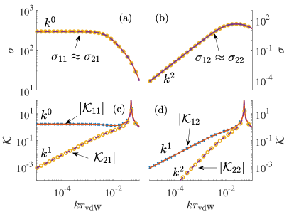
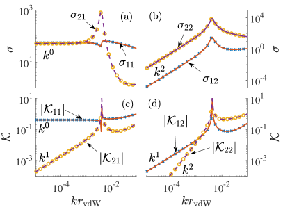
where $\underline{\mathcal{K}}^{(-)}=\tan[\delta_{p}(k_{p})]$, and $\underline{\mathcal{K}}^{(+)}$ is a $2\times 2$ matrix. The block-diagonal structure can be understood by studying the $\mathcal{\mathcal{PT}}$-symmetry of $\sum_{\nu}F_{\nu\tau}(\rho)A_{\nu}(\Omega)$ in the $m_{j}=0$ subspace, where $\mathcal{P}$ is defined as $\phi\rightarrow\phi+\pi$ and $\mathcal{T}$ is defined as $\left|s_{n},m_{n}\right\rangle\rightarrow\left|s_{n},-m_{n}\right\rangle$ for both $n=1,2$. Defining $\mathcal{P}\mathcal{T}[\sum F_{\nu\tau}(\rho)A_{\nu}(\Omega)]=\Pi_{\tau}[\sum F_{\nu\tau}(\rho)A_{\nu}(\Omega)]$, one finds that $\Pi_{\tau}=+1$ /$-1$ for $\tau=\{1,2\}$/$\{3\}$, leading to the block-diagonal structure. [For $m_{j}\neq 0$ subspaces, ${\rm sign}(m_{j})$ and $\mathcal{P}\mathcal{T}$ cannot simutaneously be good quantum numbers]. The expressions of matrix elements of $\underline{\mathcal{K}}^{(+)}$ are analytical but quite cumbersome, and hence we only give the full expression in the supplemental materials and illustrate them in Fig. 1 and Fig. 2 as two numerical examples near $s$- and $p$-wave resonances respectively. In these two examples, the energy-dependent phase-shifts $\delta_{s}(k)$ and $\delta_{p}(k)$ are obtained from a free-space scattering calculation with Lenard-Jones potential $U(\rho)=-\frac{C_{6}}{\rho^{6}}\left(1-\frac{r_{0}^{6}}{\rho^{6}}\right)$, where $C_{6}$ defines a length scale $r_{{\rm vdW}}=(2\mu_{2b}C_{6}/\hbar^{2})^{1/4}/2$ and $r_{0}$ controls short-range physics and is used to tune zero-energy scattering phase shifts. The analytical results shows a good agreement with a full numerical scatteirng calculation with the representation of SOC, using a similar procedure as Ref. (Wang et al., 2018). The technical details are shown in the Supplemental Material.

Near $s$-wave resonance, $p$-wave scattering is negligible and the scattering matrix can be simplified as

$$\underline{\mathcal{K}}^{(s)}=T_{0}\left[\begin{array}[]{cc}k_{1}&-k\\ -k&k_{2}\end{array}\right],$$

(18)

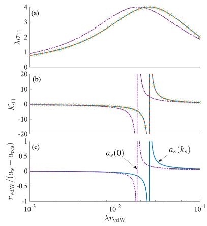
where $T_{0}=\tan[\delta_{s}(k_{s})]/2k_{b}\alpha_{s}$ and $\alpha_{s}=1+\frac{2}{\pi}\tan[\delta_{s}(k_{s})]\left(\log\frac{k}{k_{s}}+\frac{\lambda}{k_{b}}\tanh^{-1}\frac{\lambda}{k_{b}}\right)$. The $S$ matrix can be obtained via $\underline{\mathcal{S}}^{(s)}=(I+i\mathcal{\underline{\mathcal{K}}}^{(s)})(I-i\mathcal{\underline{K}}^{(s)})^{-1}$ and determines the scattering cross-section $\sigma_{\tau\tau^{\prime}}^{(s)}=2|\mathcal{\underline{S}}_{\tau\tau^{\prime}}^{(s)}-\delta_{\tau\tau^{\prime}}|^{2}/k_{\tau}$ that are read as $\sigma_{11}^{(s)}=\sigma_{21}^{(s)}=k_{1}8T_{0}^{2}/(1+4T_{0}^{2}k_{b}^{2})$ and $\sigma_{12}^{(s)}=\sigma_{22}^{(s)}=k_{2}8T_{0}^{2}/(1+4T_{0}^{2}k_{b}^{2})$. As a result, $\sigma_{21}^{(s)}/\sigma_{12}^{(s)}=k_{1}/k_{2}>1$ indicates that particles are preferentially scattered into the lower energy helicity “$-$” state. The validity of Eq. (18) near $s$-wave resonances is varified in Fig. 1. In the zero-energy limit, $\lambda\sigma_{11}^{(s)}\rightarrow 4/\left\{1+[\gamma+\frac{2}{\pi}\log\left(\lambda a_{s}(\sqrt{2}\lambda)\right)]^{2}\right\}$, where $a_{s}(k)$ is the generalized energy-dependent $s$-wave scattering length defined by $\cot[\delta_{s}(k)]=\frac{2}{\pi}\log[k_{s}a_{s}(k)]+\gamma$. The rescaled cross-section therefore reach maximum when $a_{s}(k_{s})$ equals to $a_{{\rm res}}\equiv e^{-\pi\gamma/2}/\lambda$. In comparison, if we replace $U(\rho)$ directly by ${\rm diag}[0,V_{0}^{{\rm fs}}(k,\rho),0]$, the free-space pseudopotential with $s$-wave only, and apply the Lippmann-Schwinger equation, the obtained $K$ matrix will obey the same formula Eq. (18) with $k_{s}$ replaced by $k$. Consequently, the rescaled cross-section reaches maximum when $a_{s}(0)=a_{{\rm res}}$. Figure 3 shows such comparison, where one can see the SOC-induced energy shift that leads to $k_{s}\neq k$ is crucial to chareterize the two-body scattering correctly, especially near the maximum of $\lambda\sigma_{11}$.

Near $p$-wave resonances, the $p$-wave phase shift can no longer be neglected. Neverthuless, a simplified fromula can be obtained in the low-energy limit $k\rightarrow 0$, where $\tan[\delta_{s}(k_{s})]\rightarrow-A_{s}\equiv-\tan[\delta_{s}(\sqrt{2}\lambda)]$ and $\tan[\delta_{p}(k_{p})]\rightarrow-A_{p}k^{2}$, and the $K$ matrix is given by,

$$\lim_{k\rightarrow 0}\underline{\mathcal{K}}^{(+)}=\frac{1}{d}\left[\begin{array}[]{cc}b_{11}&b_{12}k/\lambda\\ b_{21}k/\lambda&b_{22}k^{2}/\lambda^{2}\end{array}\right].$$

(19)

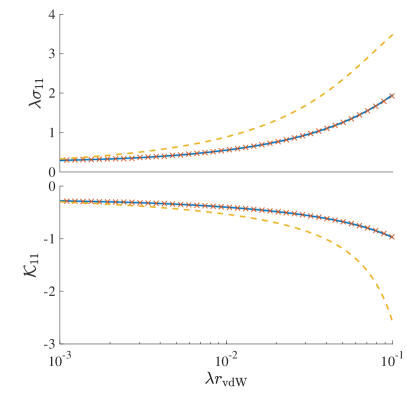
Here, $d$ and $b_{\tau^{\prime}\tau}$ are all constants, which is given by $d=1-2(\log\sqrt{2})A_{s}/\pi-2\lambda^{2}A_{p}/\pi+4\lambda^{2}A_{p}A_{s}[(\log\sqrt{2})-1]/\pi^{2}$, $b_{11}=-A_{s}(1/2-\lambda^{2}A_{p}/\pi)$, $b_{12}=b_{21}=A_{s}(1/2+\lambda^{2}A_{p}/\pi)$ and $b_{22}=-A_{s}/4-\lambda^{2}A_{p}-\lambda^{2}A_{p}A_{s}(3/2-\log 2)/\pi$. When $|\lambda^{2}A_{p}|\gtrsim 1$, $p$-wave scattering gives a significant contribution as shown in Fig. 4, where Eq. (18) is no longer valid. Neverthuless, the threshold laws for cross-section and $K$ matrix elements are valid for all situations as shown in Figs. 1 and 2. Interestingly, the elastic scattering rate $\propto k_{1}\sigma_{11}$ that determines thermalization remains constant in the zero-energy limit, in contrast to the vanishing $1/(\log k)^{2}$ rate without the presence of SOC. We also remark here that, using the free-space pseudopotential including the $p$-wave contribution ${\rm diag}[V_{1}^{{\rm fs}}(k,\rho),V_{0}^{{\rm fs}}(k,\rho),V_{1}^{{\rm fs}}(k,\rho)]$ will wrongly give a vanishingly small $K$ matrix due to a $\log(s)|_{s\rightarrow 0}$ term in the denumerator of all the matrix elements of $\underline{\mathcal{K}}^{(+)}$, reflecting the importance of the non-diagonal terms in the pseudopotnetial.

In summary, we have derived a pseudopotential in the COM frame with the presence of SOC in 2D using a frame-transformation approach. Different than the free-space pseudopotential, the s -wave scattering phase-shift changes due to a SOC-induced energy shift. The frame-transformation also introduces non-diagonal terms, which are also essential to reproduce two-body scattering observables. We applied this pseudopotential with the Lippmann-Schwinger equation to obtain the analytical scattering matrix and compare it with a numerical scattering calculation with finite-range potential. Our pseudopotential is valid even near $s$- or $p$-wave resonances as long as $\lambda r_{{\rm vdW}}\ll 1$, which is usually well satisfied in ultracold quantum gases. Our results indicate that, if we consider, if we consider $s$-wave only (which usually implies near $s$-wave resonances), and the energy-dependency of $a_{s}(k)$ is very weak (which usually implies a very broad resonance) so that $a_{s}(\sqrt{2}\lambda)\approx a_{s}(0)$, the free-space pseudopotential can give a good approximation, which gives the valid regime of previous studies in Refs. (Zhang et al., 2012c, 2013b). On the other hand, if the energy-dependency of $a_{s}(k)$ is strong or $p$-wave interaction is nonnegligible, our pseudopotential has to be adopted to reproduce two-body scattering. Our approach can also be easily applied in 3D and reproduce Eq. (11) of Ref. (Guan and Blume, 2017), which we will pursuit elsewhere. Our results are also useful for investigating universal relations and Tan’s contacts for SOC quantum gases in 2D (Cai-Xia Zhang, 2019) and might eventually be applied in many-body physics studies.

References

- Fermi (1934) E. Fermi, Nuovo Cimento 11, 157 (1934).
- Huang and Yang (1957) K. Huang and C. N. Yang, Phys. Rev. 105, 767 (1957).
- Bolda et al. (2002) E. L. Bolda, E. Tiesinga, and P. S. Julienne, Phys. Rev. A 66, 013403 (2002).
- Chin et al. (2010) C. Chin, R. Grimm, P. Julienne, and E. Tiesinga, Rev. Mod. Phys. 82, 1225 (2010).
- Lin et al. (2011) Y.-J. Lin, K. Jiménez-García, and I. B. Spielman, Nature(London) 471, 83 (2011).
- Stock et al. (2005) R. Stock, A. Silberfarb, E. L. Bolda, and I. H. Deutsch, Phys. Rev. Lett. 94, 023202 (2005).
- Derevianko (2005) A. Derevianko, Phys. Rev. A 72, 044701 (2005).
- Idziaszek and Calarco (2006) Z. Idziaszek and T. Calarco, Phys. Rev. Lett. 96, 013201 (2006).
- Roth and Feldmeier (2001) R. Roth and H. Feldmeier, Phys. Rev. A 64, 043603 (2001).
- Bloch et al. (2008) I. Bloch, J. Dalibard, and W. Zwerger, Rev. Mod. Phys. 80, 885 (2008).
- Paredes et al. (2004) B. Paredes, A. Widera, V. Murg, O. Mandel, S. Fölling, I. Cirac, G. V. Shlyapnikov, T. W. Hänsch, and I. Bloch, Nature(London) 429, 177 (2004).
- Kinoshita et al. (2004) T. Kinoshita, T. Wenger, and D. S. Weiss, Science 305, 1125 (2004).
- Hadzibabic et al. (2004) Z. Hadzibabic, P. Krüger, M. Cheneau, B. Battelier, and J. Dalibard, Science 305, 1125 (2004).
- Cladé et al. (2009) P. Cladé, C. Ryu, A. Ramanathan, K. Helmerson, and W. D. Phillips, Phys. Rev. Lett. 102, 170401 (2009).
- Rath et al. (2010) S. P. Rath, T. Yefsah, K. J. Günter, M. Cheneau, R. Desbuquois, M. Holzmann, W. Krauth, and J. Dalibard, Phys. Rev. A 82, 013609 (2010).
- Nishida et al. (2013) Y. Nishida, S. Moroz, and D. T. Son, Phys. Rev. Lett. 110, 235301 (2013).
- Gao et al. (2015) C. Gao, J. Wang, and Z. Yu, Phys. Rev. A 92, 020504 (2015).
- Kanjilal and Blume (2006) K. Kanjilal and D. Blume, Phys. Rev. A 73, 060701 (2006).
- Zhang et al. (2014) J. Zhang, H. Hu, X.-J. Liu, and H. Pu, Annu. Rev. Cold At. Mol. 2, 81 (2014).
- Zhai (2015) H. Zhai, Rep. Prog. Phys. 78, 026001 (2015).
- Dalibard et al. (2011) J. Dalibard, F. Gerbier, G. Juzeliūnas, and P. Öhberg, Rev. Mod. Phys. 83, 1523 (2011).
- Goldman et al. (2014) N. Goldman, G. Juzeliunas, P. Öhberg, and I. B. Spielman, Rep. Prog. Phys. 77, 126401 (2014).
- Struck et al. (2012) J. Struck, C. Ölschläger, M. Weinberg, P. Hauke, J. Simonet, A. Eckardt, M. Lewenstein, K. Sengstock, and P. Windpassinger, Phys. Rev. Lett. 108, 225304 (2012).
- Cheuk et al. (2012) L. W. Cheuk, A. T. Sommer, Z. Hadzibabic, T. Yefsah, W. S. Bakr, and M. W. Zwierlein, Phys. Rev. Lett. 109, 095302 (2012).
- Wang et al. (2012) P. Wang, Z.-Q. Yu, Z. Fu, J. Miao, L. Huang, S. Chai, H. Zhai, and J. Zhang, Phys. Rev. Lett. 109, 095301 (2012).
- Zhang et al. (2012a) J.-Y. Zhang, S.-C. Ji, Z. Chen, L. Zhang, Z.-D. Du, B. Yan, G.-S. Pan, B. Zhao, Y.-J. Deng, H. Zhai, S. Chen, and J.-W. Pan, Phys. Rev. Lett. 109, 115301 (2012a).
- Qu et al. (2013) C. Qu, C. Hamner, M. Gong, C. Zhang, and P. Engels, Phys. Rev. A 88, 021604 (2013).
- Khamehchi et al. (2017) M. A. Khamehchi, K. Hossain, M. E. Mossman, Y. Zhang, T. Busch, M. M. Forbes, and P. Engels, Phys. Rev. Lett. 118, 155301 (2017).
- Huang et al. (2016) L. Huang, Z. Meng, P. Wang, P. Peng, S.-L. Zhang, L. Chen, D. L. andQi Zhou, and J. Zhang, Nat. Phys. 12, 540 (2016).
- Meng et al. (2016) Z. Meng, L. Huang, P. Peng, D. Li, L. Chen, Y. Xu, C. Zhang, P. Wang, and J. Zhang, Phys. Rev. Lett. 117, 235304 (2016).
- Cui (2012) X. Cui, Phys. Rev. A 85, 022705 (2012).
- Zhang et al. (2012b) P. Zhang, L. Zhang, and Y. Deng, Phys. Rev. A 86, 053608 (2012b).
- Yu (2012) Z. Yu, Phys. Rev. A 85, 042711 (2012).
- Zhang et al. (2013a) L. Zhang, Y. Deng, and P. Zhang, Phys. Rev. A 87, 053626 (2013a).
- Duan et al. (2013) H. Duan, L. You, and B. Gao, Phys. Rev. A 87, 052708 (2013).
- Wang and Greene (2015) S.-J. Wang and C. H. Greene, Phys. Rev. A 91, 022706 (2015).
- Guan and Blume (2016) Q. Guan and D. Blume, Phys. Rev. A 94, 022706 (2016).
- Wang et al. (2018) J. Wang, C. R. Hougaard, B. C. Mulkerin, and X.-J. Liu, Phys. Rev. A 97, 042709 (2018).
- Zhang et al. (2012c) P. Zhang, L. Zhang, and W. Zhang, Phys. Rev. A 86, 042707 (2012c).
- Zhang et al. (2013b) L. Zhang, Y. Deng, and P. Zhang, Phys. Rev. A 87, 053626 (2013b).
- Guan and Blume (2017) Q. Guan and D. Blume, Phys. Rev. A 95, 020702 (2017).
- Cai-Xia Zhang (2019) K. J. Cai-Xia Zhang, Shi-Guo Peng, “Universal relations for spin-orbit-coupled fermi gases in two and three dimensions,” (2019), arXiv:1907.11433 .