This paper was converted on www.awesomepapers.org from LaTeX by an anonymous user.
Want to know more? Visit the Converter page.

Pseudo-neutrino versus recoil formalism for 4-body phase space and applications to nuclear decay

Chien-Yeah Seng1,2 1Facility for Rare Isotope Beams, Michigan State University, East Lansing, MI 48824, USA 2Department of Physics, University of Washington, Seattle, WA 98195-1560, USA
(April 3, 2025)
Abstract

It is well-known that the traditional treatment of radiative corrections that utilizes the “true” neutrino momentum pν\vec{p}_{\nu} in the differential decay rate formula could lead to a α/π\sim\alpha/\pi systematic error in certain observables due to the mistreatment of 4-body kinematics. I investigate the theory structure of one of the proposed solutions, the “ν\nu^{\prime}-formalism”, in the non-recoil limit appropriate for neutron and nuclear beta decays. I derive an elegant master formula for the 4-body phase space and use it to re-analyze the spectrum-dependent “outer” radiative corrections to the beta decay of a polarized spin-half nucleus; a complete set of analytic expressions is provided for readers to straightforwardly obtain the final numerical results. I compare it to the “recoil formalism” where the energy of the recoil nucleus is fixed.

I Introduction

Neutron and nuclear beta decays provide an excellent avenue for precision tests of the Standard Model (SM) [1, 2]. Apart from the decay lifetime that determines the Cabibbo-Kobayashi-Maskawa (CKM) matrix VudV_{ud}, the study of the beta decay spectrum and various correlations constructed from spin and momentum vectors set stringent constraints on coupling strengths induced by physics beyond the Standard Model (BSM). The first comprehensive analysis of various terms in the beta decay differential rate in terms of the parameters in the most general Lee-Yang Lagrangian [3] was done by Jackson, Treiman and Wyld  [4, 5]. Taking neutron decay as an example, the well-known tree-level differential decay rate of a polarized neutron (with unpolarized final states) reads:

(dΓdEedΩedΩν)tree1+aβp^ν+bmeEe+s^n[Aβ+Bp^ν+Dβ×p^ν],\left(\frac{d\Gamma}{dE_{e}d\Omega_{e}d\Omega_{\nu}}\right)_{\text{tree}}\propto 1+a\vec{\beta}\cdot\hat{p}_{\nu}+b\frac{m_{e}}{E_{e}}+\hat{s}_{n}\cdot\left[A\vec{\beta}+B\hat{p}_{\nu}+D\vec{\beta}\times\hat{p}_{\nu}\right]\leavevmode\nobreak\ , (1)

where p^ν\hat{p}_{\nu} is the unit neutrino momentum vector, β=pe/Ee=βp^e\vec{\beta}=\vec{p}_{e}/E_{e}=\beta\hat{p}_{e} is the electron velocity vector, and s^n\hat{s}_{n} is the neutron unit polarization vector. The SM provides well-defined predictions for the correlation coefficients aa, bb, AA and BB and DD; experimental confirmation of any deviation from such predictions will be an unambiguous signal of BSM physics.

As the present experimental precision of beta decay observables have reached 10410^{-4}, one needs to carefully account for the higher-order SM corrections to the tree-level expression; the most prominent ones are recoil effects and the radiative corrections (RC). The latter consists of the Fermi function [6] and “outer corrections” that are functions of EeE_{e} and the angles, and “inner corrections” that only serve to renormalize weak coupling constants; the first two are more important for the determination of correlation coefficients.

Pioneering works by Sirlin [7], Shann [8] and Garcia-Maya [9] established the 𝒪(α)\mathcal{O}(\alpha) outer corrections to the polarized neutron differential rate, which takes a very elegant form:

δ(dΓdEedΩedΩν)outerα2π{δ1+aβp^ν(δ1+δ2)+s^n[Aβ(δ1+δ2)+Bp^νδ1]},\delta\left(\frac{d\Gamma}{dE_{e}d\Omega_{e}d\Omega_{\nu}}\right)_{\text{outer}}\propto\frac{\alpha}{2\pi}\left\{\delta_{1}+a\vec{\beta}\cdot\hat{p}_{\nu}(\delta_{1}+\delta_{2})+\hat{s}_{n}\cdot\left[A\vec{\beta}(\delta_{1}+\delta_{2})+B\hat{p}_{\nu}\delta_{1}\right]\right\}\leavevmode\nobreak\ , (2)

where δ1\delta_{1}, δ2\delta_{2} are known functions of EeE_{e}. This equation serves as an important theory input for the study of the beta spectrum and the beta asymmetry parameter AA. On the other hand, for observables such as the neutrino-electron correlation coefficient aa and the neutrino asymmetry parameter BB, it was noticed long ago [10] that the representation above, which I call the neutrino (ν\nu)-formalism, contains a serious drawback as it depends on the neutrino momentum pν\vec{p}_{\nu} which is not directly measured. In a three-body decay ϕiϕfeν\phi_{i}\rightarrow\phi_{f}e\nu, it could be deduced from the momentum conservation pν=pfpe\vec{p}_{\nu}=-\vec{p}_{f}-\vec{p}_{e}, where both pf\vec{p}_{f} and pe\vec{p}_{e} are measurable quantities. However, this relation breaks down in the bremsstrahlung process where an extra real photon is emitted. in fact, since in most experiments the neutrino and the extra photon(s) are not directly detected, there is no way to determine the neutrino solid angle Ων\Omega_{\nu} using the momenta of ϕf\phi_{f} and ee. Putting it in other words, using the ν\nu-formalism for the differential rate together with the 3-body momentum conservation relations could lead to a theoretical error of the order α/π\alpha/\pi for the p^ν\hat{p}_{\nu}-dependent observables due to the mistreatment of the 4-body kinematics.

Several alternative approaches were proposed to overcome the drawback in Eq.(2). An important example is the “recoil formalism”, namely to fix the momenta pe\vec{p}_{e} and pf\vec{p}_{f} (instead of pe\vec{p}_{e} and pν\vec{p}_{\nu}) in the calculation; in this way one may choose the variables as Ee,EfE_{e},E_{f} or Ee,cosθefp^ep^fE_{e},\cos\theta_{ef}\equiv\hat{p}_{e}\cdot\hat{p}_{f}. This is analogous to the treatment of RC in semileptonic kaon decays [11, 12, 13, 14]. The recoil formalism was used to study decays of unpolarized [15, 16] and polarized [17, 18, 19] baryons. The complicated bremsstrahlung phase space integrals were performed either semi-analytically [16, 18] or numerically [15, 20, 21, 22]. Recently, the need to apply the correct recoil formalism (instead of the ν\nu-formalism) to the decay of free neutrons was reiterated [23], and subsequent re-analysis was performed to the aCORN [24] and aSPECT [25] data.

Another approach is the pseudo-neutrino (ν\nu^{\prime})-formalism. It defines a “pseudo-neutrino” momentum pνpepf\vec{p}_{\nu}^{\prime}\equiv-\vec{p}_{e}-\vec{p}_{f} which is a direct experimental observable; this definition holds with or without extra photons. Subsequently, one expresses the differential rate in terms of Ee,Ωe,ΩνE_{e},\Omega_{e},\Omega_{\nu}^{\prime} instead of Ee,Ωe,ΩνE_{e},\Omega_{e},\Omega_{\nu}. This approach possesses several advantageous comparing to the recoil formalism:

  • It is the most natural generalization to the traditional ν\nu-formalism and has the closest resemblance to the latter, which makes cross-checking easier. It is also the most natural formalism to describe decays of polarized nuclei.

  • It is much more natural when combined with non-recoil approximation (unlike the recoil formalism where the variation of EfE_{f} cannot be discussed without involving recoil effects). It is sometimes beneficial to study both the kinematical dynamical recoil corrections simultaneously within a unified framework, e.g. using methods like the heavy baryon expansion [26], to avoid possible double-counting. So it is desirable to split recoil effects completely from RC, and the ν\nu^{\prime}-formalism is best suited for this purpose.

  • The analytic expressions of the phase space integrals in the ν\nu^{\prime}-formalism are usually much more elegant, and only a minimal amount of numerical integration is required.

Existing literature that discussed the ν\nu^{\prime}-formalism includes Refs.[27, 17, 18, 16], with applications to decays of unpolarized and polarized neutron and hyperons. Despite their comprehensiveness, I failed to identify a complete treatment of the outer RC to the differential rate of a polarized parent nucleus in the non-recoil limit (appropriate for neutron and nuclear decays) with the ν\nu^{\prime}-formalism which, in principle, should display a similar degree of theory elegance as Eq.(2). Also, analytic expressions of many important intermediate quantities (e.g. expansion coefficients and results of phase-space integrals) are not explicitly shown, which makes their results not so straightforwardly applicable in numerical analysis; furthermore, one also finds that some numerical results in these earlier papers are not completely accurate. In the meantime, while many recent computer packages are capable to produce reliable numerical results [23], they are practically a black box to outsiders.

The purpose of this paper is to provide a transparent, elegant and self-contained theoretical description of the ν\nu^{\prime}-formalism in the non-recoil limit. As a simple application, I study the outer RC to the differential rate of the β±\beta^{\pm} decay of a polarized spin-1/2 nucleus, but the final result is equally applicable to spin-0 systems. Therefore, this analysis covers a wide range of interesting beta decay processes including semileptonic pion decay, free neutron decay, superallowed 0+0+0^{+}\rightarrow 0^{+} decays [28], spin-half nuclear mirror transitions [29] (e.g. 19Ne\rightarrow19F), etc. I provide the full set of analytic expressions of all intermediate functions needed in the analysis, so that the quoted numerical results are fully transparent and can be easily reproduced by any interested reader, without the need of complicated numerical packages. For completeness, I also provide a similar set of analytic formula for unpolarized nuclei in the recoil formalism.

II 3-body phase space

I start by briefly reviewing the total rate formula of a 3-body decay ϕi(pi)ϕf(pf)+e(pe)+ν(pν)\phi_{i}(p_{i})\rightarrow\phi_{f}(p_{f})+e(p_{e})+\nu(p_{\nu})111The term “electron” throughout this paper may refer to an electron or a positron depending on the decay mode, and similar for the neutrino.:

Γ3=𝑑Π3||3-body2\Gamma_{3}=\int d\Pi_{3}|\mathcal{M}|_{\text{3-body}}^{2} (3)

with the 3-body phase space:

𝑑Π3=12mid3pf(2π)32Efd3pe(2π)32Eed3pν(2π)32Eν(2π)4δ(4)(pipfpepν).\int d\Pi_{3}=\frac{1}{2m_{i}}\int\frac{d^{3}p_{f}}{(2\pi)^{3}2E_{f}}\frac{d^{3}p_{e}}{(2\pi)^{3}2E_{e}}\frac{d^{3}p_{\nu}}{(2\pi)^{3}2E_{\nu}}(2\pi)^{4}\delta^{(4)}(p_{i}-p_{f}-p_{e}-p_{\nu})\leavevmode\nobreak\ . (4)

One is interested in beta decay processes where mi,mfmimfm_{i},m_{f}\gg m_{i}-m_{f}. The evaluation of this phase space in the ν\nu-formalism consists of first integrating out pf\vec{p}_{f} using the spatial delta function. The remaining temporal delta function reads:

δ(miEfEeEν)δ(EmEeEν)\delta(m_{i}-E_{f}-E_{e}-E_{\nu})\approx\delta(E_{m}-E_{e}-E_{\nu}) (5)

which only set bounds on the energy variables but not the angles; here I have taken the non-recoil approximation, EfmfE_{f}\approx m_{f} and Em(mi2mf2+me2)/(2mi)mimfE_{m}\equiv(m_{i}^{2}-m_{f}^{2}+m_{e}^{2})/(2m_{i})\approx m_{i}-m_{f} is the electron end-point energy. Of course, in practice one needs to account for recoil corrections to the tree-level 3-body rate for precision, but that is not the focus of this paper. This delta function is then used to integrate out the neutrino energy, which leaves us with:

𝑑Π31512π5mimf𝑑Ωe𝑑ΩνmeEm𝑑Ee|pe|Eν,\int d\Pi_{3}\approx\frac{1}{512\pi^{5}m_{i}m_{f}}\int d\Omega_{e}d\Omega_{\nu}\int_{m_{e}}^{E_{m}}dE_{e}|\vec{p}_{e}|E_{\nu}\leavevmode\nobreak\ , (6)

where Eν=EmEeE_{\nu}=E_{m}-E_{e}; the upper limit of EeE_{e} is set by the temporal delta function: EmEe=Eν0E_{m}-E_{e}=E_{\nu}\geq 0. Eq.(6) is the underlying reason why one utilized EeE_{e}, Ωe\Omega_{e} and Ων\Omega_{\nu} as free variables in the traditional analysis of beta decays.

To bypass the conceptual deficit in the ν\nu-formalism that Ων\Omega_{\nu} is not a practical observable, one may turn to the ν\nu^{\prime}-formalism by defining the pseudo-neutrino momentum:

pνpipfpe=(Eν,pν)p_{\nu}^{\prime}\equiv p_{i}-p_{f}-p_{e}=(E_{\nu}^{\prime},\vec{p}_{\nu}^{\prime}) (7)

which is an experimental observable, because both ee and ϕf\phi_{f} can be directly detected. In the non-recoil limit, Eν=EmEeE_{\nu}^{\prime}=E_{m}-E_{e} is only a function of electron energy. In this formalism, I change the integration over pf\vec{p}_{f} to that over pν\vec{p}_{\nu}^{\prime}:

d3pfd3pe=d3pνd3pe,\int d^{3}p_{f}d^{3}p_{e}=\int d^{3}p_{\nu}^{\prime}d^{3}p_{e}\leavevmode\nobreak\ , (8)

and rewrite Eq.(4) in the non-recoil limit as:

𝑑Π31(2π)68mimfd3pνd3peEed3pν(2π)32Eν(2π)4δ(4)(pνpν),\int d\Pi_{3}\approx\frac{1}{(2\pi)^{6}8m_{i}m_{f}}\int d^{3}p_{\nu}^{\prime}\frac{d^{3}p_{e}}{E_{e}}\frac{d^{3}p_{\nu}}{(2\pi)^{3}2E_{\nu}}(2\pi)^{4}\delta^{(4)}(p_{\nu}^{\prime}-p_{\nu})\leavevmode\nobreak\ , (9)

and integrate out pν\vec{p}_{\nu}, instead of pf\vec{p}_{f}, using the spatial delta function. The remaining temporal delta function reads δ(Eν|pν|)\delta(E_{\nu}^{\prime}-|\vec{p}_{\nu}^{\prime}|), which is then used to integrate out |pν||\vec{p}_{\nu}^{\prime}|. This yields:

𝑑Π31512π5mimf𝑑Ωe𝑑ΩνmeEm𝑑Ee|pe|Eν.\int d\Pi_{3}\approx\frac{1}{512\pi^{5}m_{i}m_{f}}\int d\Omega_{e}d\Omega_{\nu}^{\prime}\int_{m_{e}}^{E_{m}}dE_{e}|\vec{p}_{e}|E_{\nu}^{\prime}\leavevmode\nobreak\ . (10)

This is identical to Eq.(6) upon replacing EνEνE_{\nu}^{\prime}\rightarrow E_{\nu} and ΩνΩν\Omega_{\nu}^{\prime}\rightarrow\Omega_{\nu}, which do not change the physics since pν=pνp_{\nu}^{\prime}=p_{\nu} in 3-body decay. The real distinction between the two formalisms only shows up when extra photons are emitted.

To facilitate the discussion later, I also provide the representation of the 3-body phase space in the recoil formalism, i.e. using EeE_{e} and EfE_{f} as variables. It is most convenient to adopt the notations used in semileptonic decays of kaons [11, 12, 13, 14], where the differential decay rate is expressed in terms of the following dimensionless Lorentz scalars:

xpν2mi2,y2pipemi2,z2pipfmi2,x\equiv\frac{p_{\nu}^{\prime 2}}{m_{i}^{2}}\leavevmode\nobreak\ ,\leavevmode\nobreak\ y\equiv\frac{2p_{i}\cdot p_{e}}{m_{i}^{2}}\leavevmode\nobreak\ ,\leavevmode\nobreak\ z\equiv\frac{2p_{i}\cdot p_{f}}{m_{i}^{2}}\leavevmode\nobreak\ , (11)

with y=2Ee/miy=2E_{e}/m_{i} and z=2Ef/miz=2E_{f}/m_{i} energy parameters in the parent’s rest frame. In 3-body decay, pν2=pν2=0p_{\nu}^{\prime 2}=p_{\nu}^{2}=0 assuming massless neutrino, and I obtain the exact relation:

𝑑Π3=mi256π3𝒟3𝑑y𝑑z,\int d\Pi_{3}=\frac{m_{i}}{256\pi^{3}}\int_{\mathcal{D}_{3}}dydz\leavevmode\nobreak\ , (12)

where the integration region 𝒟3\mathcal{D}_{3} can be represented in two equivalent ways:

a(y)b(y)<z<a(y)+b(y),\displaystyle a(y)-b(y)<z<a(y)+b(y)\leavevmode\nobreak\ , 2re<y<1+rerf\displaystyle 2\sqrt{r_{e}}<y<1+r_{e}-r_{f}
a(y)=(2y)(1+rf+rey)2(1+rey),\displaystyle a(y)=\frac{(2-y)(1+r_{f}+r_{e}-y)}{2(1+r_{e}-y)}\leavevmode\nobreak\ , b(y)=y24re(1+rerfy)2(1+rey),\displaystyle b(y)=\frac{\sqrt{y^{2}-4r_{e}}(1+r_{e}-r_{f}-y)}{2(1+r_{e}-y)}\leavevmode\nobreak\ , (13)

or

c(z)d(z)<y<c(z)+d(z),\displaystyle c(z)-d(z)<y<c(z)+d(z)\leavevmode\nobreak\ , 2rf<z<1+rfre\displaystyle 2\sqrt{r_{f}}<z<1+r_{f}-r_{e}
c(z)=(2z)(1+re+rfz)2(1+rfz),\displaystyle c(z)=\frac{(2-z)(1+r_{e}+r_{f}-z)}{2(1+r_{f}-z)}\leavevmode\nobreak\ , d(z)=z24rf(1+rfrez)2(1+rfz),\displaystyle d(z)=\frac{\sqrt{z^{2}-4r_{f}}(1+r_{f}-r_{e}-z)}{2(1+r_{f}-z)}\leavevmode\nobreak\ , (14)

with rfmf2/mi2r_{f}\equiv m_{f}^{2}/m_{i}^{2}, reme2/mi2r_{e}\equiv m_{e}^{2}/m_{i}^{2}.

III 4-body phase space

The contribution from the bremsstrahlung process ϕi(pi)ϕf(pf)+e(pe)+ν(pν)+γ(k)\phi_{i}(p_{i})\rightarrow\phi_{f}(p_{f})+e(p_{e})+\nu(p_{\nu})+\gamma(k) to the total decay rate is:

Γ4=𝑑Π4||4-body2,\Gamma_{4}=\int d\Pi_{4}|\mathcal{M}|^{2}_{\text{4-body}}\leavevmode\nobreak\ , (15)

where the 4-body phase space reads:

𝑑Π4=12mid3pf(2π)32Efd3pe(2π)32Eed3pν(2π)32Eνd3k(2π)32Ek(2π)4δ(4)(pipfpepνk).\int d\Pi_{4}=\frac{1}{2m_{i}}\int\frac{d^{3}p_{f}}{(2\pi)^{3}2E_{f}}\frac{d^{3}p_{e}}{(2\pi)^{3}2E_{e}}\frac{d^{3}p_{\nu}}{(2\pi)^{3}2E_{\nu}}\frac{d^{3}k}{(2\pi)^{3}2E_{k}}(2\pi)^{4}\delta^{(4)}(p_{i}-p_{f}-p_{e}-p_{\nu}-k)\leavevmode\nobreak\ . (16)

Let us again evaluate the phase space first in the traditional ν\nu-formalism. I integrate out pf\vec{p}_{f} using the spatial delta function, which leaves the temporal part as:

δ(miEfEeEνEk)δ(EmEeEνEk).\delta(m_{i}-E_{f}-E_{e}-E_{\nu}-E_{k})\approx\delta(E_{m}-E_{e}-E_{\nu}-E_{k})\leavevmode\nobreak\ . (17)

Here the non-recoil approximation can be safely taken, because in neutron/nuclear beta decays a recoil correction on top of a RC gives a (α/π)(mimf)/mi105\sim(\alpha/\pi)(m_{i}-m_{f})/m_{i}\lesssim 10^{-5} correction to the total decay rate, which exceeds the experimental precision and can be neglected. The remaining delta function is then used to integrate out EνE_{\nu}, which gives:

𝑑Π41512π5mimf𝑑Ωe𝑑ΩνmeEm𝑑Ee|pe|Ek<EmEed3k(2π)32EkEν,\int d\Pi_{4}\approx\frac{1}{512\pi^{5}m_{i}m_{f}}\int d\Omega_{e}d\Omega_{\nu}\int_{m_{e}}^{E_{m}}dE_{e}|\vec{p}_{e}|\int_{E_{k}<E_{m}-E_{e}}\frac{d^{3}k}{(2\pi)^{3}2E_{k}}E_{\nu}\leavevmode\nobreak\ , (18)

where Eν=EmEeEkE_{\nu}=E_{m}-E_{e}-E_{k}. The unobserved photon momentum k\vec{k} is then integrated out, leaving EeE_{e}, Ωe\Omega_{e} and Ων\Omega_{\nu} as variables in the differential decay rate formula.

As I stressed in the introduction, since in Eq.(18) the unobserved photon momentum is integrated out, further applying the 3-body momentum conservation pν=pipfpep_{\nu}=p_{i}-p_{f}-p_{e} to the 4-body phase space in the ν\nu-formalism leads to an error. This issue is non-existent in the recoil formalism, since the variables {x,y,z}\{x,y,z\} are experimentally measurable. In this formalism, one can derive the following exact formula of the 4-body phase space [30]:

𝑑Π4\displaystyle\int d\Pi_{4} =\displaystyle= mi3512π4{𝒟3𝑑y𝑑z0α+(y,z)𝑑x+𝒟43𝑑y𝑑zα(y,z)α+(y,z)𝑑x}d3k(2π)32Ekd3pν(2π)32Eν\displaystyle\frac{m_{i}^{3}}{512\pi^{4}}\left\{\int_{\mathcal{D}_{3}}dydz\int_{0}^{\alpha_{+}(y,z)}dx+\int_{\mathcal{D}_{4-3}}dydz\int_{\alpha_{-}(y,z)}^{\alpha_{+}(y,z)}dx\right\}\int\frac{d^{3}k}{(2\pi)^{3}2E_{k}}\frac{d^{3}p_{\nu}}{(2\pi)^{3}2E_{\nu}} (19)
×(2π)4δ(4)(pνpνk),\displaystyle\times(2\pi)^{4}\delta^{(4)}(p_{\nu}^{\prime}-p_{\nu}-k)\leavevmode\nobreak\ ,

where

α±(y,z)1yz+rf+re+yz2±12y24rez24rf,\alpha_{\pm}(y,z)\equiv 1-y-z+r_{f}+r_{e}+\frac{yz}{2}\pm\frac{1}{2}\sqrt{y^{2}-4r_{e}}\sqrt{z^{2}-4r_{f}}\leavevmode\nobreak\ , (20)

and the region 𝒟43\mathcal{D}_{4-3} can also be expressed in two equivalent ways:

2rf<z<a(y)b(y), 2re<y<1rf+re1rf2\sqrt{r_{f}}<z<a(y)-b(y)\leavevmode\nobreak\ ,\leavevmode\nobreak\ 2\sqrt{r_{e}}<y<1-\sqrt{r_{f}}+\frac{r_{e}}{1-\sqrt{r_{f}}} (21)

or

2re<y<c(z)d(z), 2rf<z<1re+rf1re.2\sqrt{r_{e}}<y<c(z)-d(z)\leavevmode\nobreak\ ,\leavevmode\nobreak\ 2\sqrt{r_{f}}<z<1-\sqrt{r_{e}}+\frac{r_{f}}{1-\sqrt{r_{e}}}\leavevmode\nobreak\ . (22)

This formula is extremely useful, because it turns out the pνp_{\nu}- and kk-integration with respect to the squared amplitude is always analytically doable [13], so one is left with at most one single numerical integration over xx, if the differential rate is expressed as dΓ/dydzd\Gamma/dydz. The recoil formalism has also been applied to baryon decays [15, 16, 17, 18, 19]; in particular, the non-overlapping regions 𝒟3\mathcal{D}_{3} and 𝒟43\mathcal{D}_{4-3} in Eq.(19) are just what known as the “in” and “out” region respectively in Ref.[23]. However, since {y,z}\{y,z\} are all energy and not angular variables, the connection to the traditional representation (1), (2) is not straightforward.

To overcome the aforementioned shortcomings, I re-evaluate the 4-body phase space in the ν\nu^{\prime}-formalism, keeping close analogy to the 3-body case as well as the kaon representation, in order to retain the advantages in both methods. Notice that the definition of the pseudo-neutrino momentum pνp_{\nu}^{\prime} in Eq.(7) remains unchanged in 4-body, and the relation Eν=EmEeE_{\nu}^{\prime}=E_{m}-E_{e} still holds. I first write:

d3pfd3peEe=d3pνd3peEe=𝑑Ωe𝑑Ων𝑑Ee|pe|d|pν||pν|2,\int d^{3}p_{f}\frac{d^{3}p_{e}}{E_{e}}=\int d^{3}p_{\nu}^{\prime}\frac{d^{3}p_{e}}{E_{e}}=\int d\Omega_{e}d\Omega_{\nu}^{\prime}\int dE_{e}|\vec{p}_{e}|\int d|\vec{p}_{\nu}^{\prime}||\vec{p}_{\nu}^{\prime}|^{2}\leavevmode\nobreak\ , (23)

and deduce the boundaries of each variable. First, the boundaries of EeE_{e}, Ωe\Omega_{e} and Ων\Omega_{\nu}^{\prime} must be exactly the same as in the 3-body case; an easy way to understand this is that it must be so to ensure the exact cancellation of the infrared (IR)-divergence between the 3-body (one-loop) and 4-body (tree-level) contributions to the differential decay rate dΓ/dEedΩedΩνd\Gamma/dE_{e}d\Omega_{e}d\Omega_{\nu}^{\prime} [31, 32, 33, 34, 35]. The boundaries of |pν||\vec{p}_{\nu}^{\prime}| are determined by the delta function:

pν2=Eν2|pν|2=(pν+k)2=(Eν+Ek)2|pν+k|20,p_{\nu}^{\prime 2}=E_{\nu}^{\prime 2}-|\vec{p}_{\nu}^{\prime}|^{2}=(p_{\nu}+k)^{2}=(E_{\nu}+E_{k})^{2}-|\vec{p}_{\nu}+\vec{k}|^{2}\geq 0\leavevmode\nobreak\ , (24)

so one has |pν|Eν|\vec{p}_{\nu}^{\prime}|\leq E_{\nu}^{\prime}, with the equal sign occurring when pνk\vec{p}_{\nu}\parallel\vec{k}. Meanwhile, for any given pe\vec{p}_{e}, a pν=0\vec{p}_{\nu}^{\prime}=\vec{0} configuration can always be achieved by setting pf=pe\vec{p}_{f}=-\vec{p}_{e} (which does not affect the energy EfmfE_{f}\approx m_{f} in the non-recoil limit), with the remaining energy of the system carried away by a νγ\nu\gamma-pair with equal and opposite momenta. So, the lower and upper limits of the |pν||\vec{p}_{\nu}^{\prime}|-integration are 0 and EνE_{\nu}^{\prime} respectively. Thus, I obtain the ν\nu^{\prime}-representation of the 4-body phase space in the non-recoil limit:

𝑑Π4\displaystyle\int d\Pi_{4} \displaystyle\approx 1512π6mimf𝑑Ωe𝑑ΩνmeEm𝑑Ee|pe|0Eνd|pν||pν|2d3k(2π)32Ekd3pν(2π)32Eν\displaystyle\frac{1}{512\pi^{6}m_{i}m_{f}}\int d\Omega_{e}d\Omega_{\nu}^{\prime}\int_{m_{e}}^{E_{m}}dE_{e}|\vec{p}_{e}|\int_{0}^{E_{\nu}^{\prime}}d|\vec{p}_{\nu}^{\prime}||\vec{p}_{\nu}^{\prime}|^{2}\int\frac{d^{3}k}{(2\pi)^{3}2E_{k}}\frac{d^{3}p_{\nu}}{(2\pi)^{3}2E_{\nu}} (25)
×(2π)4δ(4)(pνpνk).\displaystyle\times(2\pi)^{4}\delta^{(4)}(p_{\nu}^{\prime}-p_{\nu}-k)\leavevmode\nobreak\ .

Eq.(25) is the first central result of this work. It possesses the following advantages:

  1. 1.

    The differential rate is expressible in terms of the experimentally-measurable energy and angular variables EeE_{e}, Ωe\Omega_{e} and Ων\Omega_{\nu}^{\prime}, which solves the problem in the traditional ν\nu-formalism.

  2. 2.

    The mathematical structure of Eq.(25) is much more elegant than the recoil formalism, Eq.(19). For instance, here one does not need to separate the so-called “in” and “out” region as two different terms, and the boundaries are also much simpler.

  3. 3.

    The full pνp_{\nu}- and kk-integrations are retained as in the kaon formalism. This allows one to directly make use of the known analytic formula of such integrations in the latter.

Finally, one can easily check the correctness of Eq.(25) by comparing it to Eq.(19). For instance, after removing the pνp_{\nu}- and kk-measures and the delta function, I evaluate the two expressions numerically by substituting the neutron decay parameters, and find that their difference is at the level 0.1% which is the typical size of a recoil correction (mnmp)/mn\sim(m_{n}-m_{p})/m_{n}. This shows that Eq.(25) is indeed the correct 4-body phase space formula in the non-recoil limit.

IV Radiative corrections to nuclear decay in ν\nu^{\prime}-formalism

As an important application of the ν\nu^{\prime}-formalism, I study the so-called “outer RC” in a Ji=Jf=1/2J_{i}=J_{f}=1/2 decay of a polarized parent nucleus (with unmeasured final spins) at the 𝒪(α/π)\mathcal{O}(\alpha/\pi) level. This includes well-known one-loop corrections and the one-photon bremsstrahlung process. The former does not distinguish between the ν\nu- and ν\nu^{\prime}-method, so I focus on the latter.

I start by writing down the hadronic and leptonic charged weak current operator222In this work I adopt the experimentalists’ convention, gA<0g_{A}<0.:

Jhadμ={n¯γμ(gV+gAγ5)p,β+p¯γμ(gV+gAγ5)n,β,Jlepμ={ν¯γμ(1γ5)e,β+e¯γμ(1γ5)ν,β.J_{\text{had}}^{\mu}=\left\{\begin{array}[]{ccc}\bar{n}\gamma^{\mu}(g_{V}+g_{A}\gamma_{5})p&,&\beta^{+}\\ \bar{p}\gamma^{\mu}(g_{V}+g_{A}\gamma_{5})n&,&\beta^{-}\end{array}\right.\leavevmode\nobreak\ ,\leavevmode\nobreak\ J_{\text{lep}}^{\mu}=\left\{\begin{array}[]{ccc}\bar{\nu}\gamma^{\mu}(1-\gamma_{5})e&,&\beta^{+}\\ \bar{e}\gamma^{\mu}(1-\gamma_{5})\nu&,&\beta^{-}\end{array}\right.\leavevmode\nobreak\ . (26)

The Fermi (F) and Gamow-Teller (GT) matrix element of JhadμJ_{\text{had}}^{\mu} are defined through:

f|d3xJhad0(x)|i=gVMF𝟙,f|d3xJhad(x)|i=gA3MGTσ.\langle f|\int d^{3}xJ_{\text{had}}^{0}(\vec{x})|i\rangle=g_{V}M_{\text{F}}\mathbbm{1}\leavevmode\nobreak\ ,\leavevmode\nobreak\ \langle f|\int d^{3}x\vec{J}_{\text{had}}(\vec{x})|i\rangle=\frac{g_{A}}{\sqrt{3}}M_{\text{GT}}\vec{\sigma}\leavevmode\nobreak\ . (27)

With this one can define a “generalized” axial-to-vector ratio:

λMGT3MFgAgV,\lambda\equiv\frac{M_{\text{GT}}}{\sqrt{3}M_{\text{F}}}\frac{g_{A}}{g_{V}}\leavevmode\nobreak\ , (28)

which reduces to gA/gVg_{A}/g_{V} for neutron decay (MF=1M_{\text{F}}=1 and MGT=3M_{\text{GT}}=\sqrt{3}). Taking the non-recoil limit at the amplitude level, which corresponds to setting pfpip=(m,0)p_{f}\approx p_{i}\equiv p=(m,\vec{0}) with m=mim=m_{i} for simplicity, I can write down the tree-level squared amplitude as:

||tree216GV2m2EeEν{1+3λ2+(1λ2)βp^ν+s^[2λ(λζ1)β2λ(λζ+1)p^ν]},|\mathcal{M}|_{\text{tree}}^{2}\approx 16G_{V}^{2}m^{2}E_{e}E_{\nu}^{\prime}\left\{1+3\lambda^{2}+(1-\lambda^{2})\vec{\beta}\cdot\hat{p}_{\nu}^{\prime}+\hat{s}\cdot\left[2\lambda(\lambda\zeta-1)\vec{\beta}-2\lambda(\lambda\zeta+1)\hat{p}_{\nu}^{\prime}\right]\right\}\leavevmode\nobreak\ , (29)

where ζ=+1(1)\zeta=+1(-1) for β+(β)\beta^{+}(\beta^{-})-decay, GVGFVudgVMFG_{V}\equiv G_{F}V_{ud}g_{V}M_{F} is the effective weak vector coupling, and s^\hat{s} is the unit vector of the parent’s polarization. Plugging it into Eq.(10) gives the tree-level differential rate in the non-recoil limit (taking m2mimfm^{2}\approx m_{i}m_{f}):

(dΓdEedΩedΩν)tree\displaystyle\left(\frac{d\Gamma}{dE_{e}d\Omega_{e}d\Omega_{\nu}^{\prime}}\right)_{\text{tree}} \displaystyle\approx GV2(2π)5|pe|EeEν2{1+3λ2+(1λ2)βp^ν\displaystyle\frac{G_{V}^{2}}{(2\pi)^{5}}|\vec{p}_{e}|E_{e}E_{\nu}^{\prime 2}\Bigl{\{}1+3\lambda^{2}+(1-\lambda^{2})\vec{\beta}\cdot\hat{p}_{\nu}^{\prime} (30)
+s^[2λ(λζ1)β2λ(λζ+1)p^ν]}.\displaystyle+\hat{s}\cdot\left[2\lambda(\lambda\zeta-1)\vec{\beta}-2\lambda(\lambda\zeta+1)\hat{p}_{\nu}^{\prime}\right]\Bigr{\}}\leavevmode\nobreak\ .

IV.1 The bremsstrahlung squared amplitude

Refer to caption
Figure 1: Bremsstrahlung diagrams.

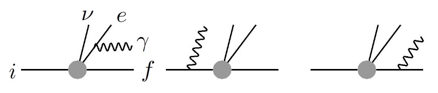
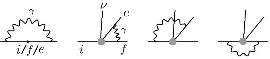
I now write down the bremsstrahlung amplitude deduced from the Feynman diagrams in Fig.1. I express it in a relativistic form, but again take take the non-recoil limit to the amplitude, which gives:

\displaystyle\mathcal{M} \displaystyle\approx GVe2ζ(pεpkpeεpek)HμLμGVe2(ζ(kμενkνεμ)+iϵμναβkαεβ2pek)HμLν\displaystyle\frac{G_{V}e}{\sqrt{2}}\zeta\left(\frac{p\cdot\varepsilon^{*}}{p\cdot k}-\frac{p_{e}\cdot\varepsilon^{*}}{p_{e}\cdot k}\right)H_{\mu}L^{\mu}-\frac{G_{V}e}{\sqrt{2}}\left(\frac{\zeta(k^{\mu}\varepsilon^{*\nu}-k^{\nu}\varepsilon^{*\mu})+i\epsilon^{\mu\nu\alpha\beta}k_{\alpha}\varepsilon_{\beta}^{*}}{2p_{e}\cdot k}\right)H_{\mu}L_{\nu} (31)
\displaystyle\equiv I+II.\displaystyle\mathcal{M}_{\text{I}}+\mathcal{M}_{\text{II}}\leavevmode\nobreak\ .

where

Hμ=u¯f(p)γμ(1+λγ5)ui(p),Lμ={u¯ν(pν)γμ(1γ5)ve(pe),β+u¯e(pe)γμ(1γ5)vν(pν),βH_{\mu}=\bar{u}_{f}(p)\gamma_{\mu}(1+\lambda\gamma_{5})u_{i}(p)\leavevmode\nobreak\ ,\leavevmode\nobreak\ L_{\mu}=\left\{\begin{array}[]{ccc}\bar{u}_{\nu}(p_{\nu})\gamma_{\mu}(1-\gamma_{5})v_{e}(p_{e})&,&\beta^{+}\\ \bar{u}_{e}(p_{e})\gamma_{\mu}(1-\gamma_{5})v_{\nu}(p_{\nu})&,&\beta^{-}\end{array}\right. (32)

are the hadronic and leptonic matrix elements of the charged weak current, respectively. Summing over the final spins leads to the following hadronic and leptonic tensors:

Hμν\displaystyle H_{\mu\nu} \displaystyle\equiv sfHμHν=Tr[(+m)γμ(1+λγ5)Σi(+m)γν(1+λγ5)]\displaystyle\sum_{s_{f}}H_{\mu}H_{\nu}^{*}=\text{Tr}[(\not{p}+m)\gamma_{\mu}(1+\lambda\gamma_{5})\Sigma_{i}(\not{p}+m)\gamma_{\nu}(1+\lambda\gamma_{5})]
Lμν\displaystyle L_{\mu\nu} \displaystyle\equiv se,sνLμLν=8{gμνpepν+peμ(pν)ν+peν(pν)μiζϵαβμνpeαpνβ},\displaystyle\sum_{s_{e},s_{\nu}}L_{\mu}L_{\nu}^{*}=8\left\{-g_{\mu\nu}p_{e}\cdot p_{\nu}+p_{e\mu}(p_{\nu})_{\nu}+p_{e\nu}(p_{\nu})_{\mu}-i\zeta\epsilon_{\alpha\beta\mu\nu}p_{e}^{\alpha}p_{\nu}^{\beta}\right\}\leavevmode\nobreak\ , (33)

where Σi(1+γ5)/2\Sigma_{i}\equiv(1+\gamma_{5}\not{s})/2 is the parent’s spin projection operator, with sμ=(0,s^)s^{\mu}=(0,\hat{s}) the parent’s spin vector. In what follows, the sum over all final spins is always assumed in the squared amplitude.

The square of I\mathcal{M}_{\text{I}} needs some extra care:

|I|2=GV2e22(ppkpepek)2HμνLμν|I|a2+|I|b2,|\mathcal{M}_{\text{I}}|^{2}=-\frac{G_{V}^{2}e^{2}}{2}\left(\frac{p}{p\cdot k}-\frac{p_{e}}{p_{e}\cdot k}\right)^{2}H_{\mu\nu}L^{\mu\nu}\equiv|\mathcal{M}_{\text{I}}|^{2}_{a}+|\mathcal{M}_{\text{I}}|^{2}_{b}\leavevmode\nobreak\ , (34)

where I split the “true” neutrino momentum as pν=pνkp_{\nu}=p_{\nu}^{\prime}-k, and pν(k)p_{\nu}^{\prime}(-k) gives the a(b)a(b) term respectively; it turns out that the (a)(a) term is the only piece that gives rise to an IR-divergence upon the phase-space integration. So, one can split the full squared amplitude into an IR-divergent piece and a regular piece: ||2=|I|a2+||reg2|\mathcal{M}|^{2}=|\mathcal{M}_{\text{I}}|^{2}_{a}+|\mathcal{M}|^{2}_{\text{reg}}, where

||reg2=|I|b2+2𝔢{III}+|II|2.|\mathcal{M}|^{2}_{\text{reg}}=|\mathcal{M}_{\text{I}}|^{2}_{b}+2\mathfrak{Re}\{\mathcal{M}_{\text{I}}\mathcal{M}_{\text{II}}^{*}\}+|\mathcal{M}_{\text{II}}|^{2}\leavevmode\nobreak\ . (35)

IV.2 “Analytic” part of the outer RC

Next I plug the squared amplitude into the 4-body decay rate formula in the ν\nu^{\prime}-formalism, i.e. Eqs.(15), (25). To evaluate the IR-divergent bremsstrahlung contribution I spell out the dot products in |I|a2|\mathcal{M}_{\text{I}}|_{a}^{2}:

|I|a2\displaystyle|\mathcal{M}_{\text{I}}|_{a}^{2} =\displaystyle= 16GV2e2m2EeEν(ppkpepek)2{1+3λ2+(1λ2)(1+|pν|EνEν)βp^ν\displaystyle-16G_{V}^{2}e^{2}m^{2}E_{e}E_{\nu}^{\prime}\left(\frac{p}{p\cdot k}-\frac{p_{e}}{p_{e}\cdot k}\right)^{2}\left\{1+3\lambda^{2}+(1-\lambda^{2})\left(1+\frac{|\vec{p}_{\nu}^{\prime}|-E_{\nu}^{\prime}}{E_{\nu}^{\prime}}\right)\vec{\beta}\cdot\hat{p}_{\nu}^{\prime}\right. (36)
+s^[2λ(λζ1)β2λ(λζ+1)(1+|pν|EνEν)p^ν]},\displaystyle\left.+\hat{s}\cdot\left[2\lambda(\lambda\zeta-1)\vec{\beta}-2\lambda(\lambda\zeta+1)\left(1+\frac{|\vec{p}_{\nu}^{\prime}|-E_{\nu}^{\prime}}{E_{\nu}^{\prime}}\right)\hat{p}_{\nu}^{\prime}\right]\right\}\leavevmode\nobreak\ ,

where p^νpν/|pν|\hat{p}_{\nu}^{\prime}\equiv\vec{p}_{\nu}^{\prime}/|\vec{p}_{\nu}^{\prime}| is the unit pseudo-neutrino momentum vector. I plug it into Eqs.(15), (25), and the explicit dependence of pνp_{\nu}, kk and |pν||\vec{p}_{\nu}^{\prime}| in the expression above allows us to integrate them analytically using the formula in Appendix A. That gives the following correction to the differential rate :

δ(dΓdEedΩedΩν)(I.a)\displaystyle\delta\left(\frac{d\Gamma}{dE_{e}d\Omega_{e}d\Omega_{\nu}^{\prime}}\right)_{(\text{I}.a)} =\displaystyle= GV2(2π)5|pe|EeEν2α2π{(1+3λ2)δIa1+(1λ2)(δIa1+δIa2)βp^ν\displaystyle\frac{G_{V}^{2}}{(2\pi)^{5}}|\vec{p}_{e}|E_{e}E_{\nu}^{\prime 2}\frac{\alpha}{2\pi}\left\{(1+3\lambda^{2})\delta_{\text{I}a1}+(1-\lambda^{2})(\delta_{\text{I}a1}+\delta_{\text{I}a2})\vec{\beta}\cdot\hat{p}_{\nu}^{\prime}\right. (37)
+s^[2λ(λζ1)δIa1β2λ(λζ+1)(δIa1+δIa2)p^ν]}.\displaystyle\left.+\hat{s}\cdot\left[2\lambda(\lambda\zeta-1)\delta_{\text{I}a1}\vec{\beta}-2\lambda(\lambda\zeta+1)(\delta_{\text{I}a1}+\delta_{\text{I}a2})\hat{p}_{\nu}^{\prime}\right]\right\}\leavevmode\nobreak\ .

The function δIa1\delta_{\text{I}a1} contains an IR-divergence regularized by a fictitious photon mass mγm_{\gamma}, which is exactly canceled with that in the virtual outer correction, see Appendix B. Combining these two pieces yields the “analytic” part of the outer RC:

δ(dΓdEedΩedΩν)v+δ(dΓdEedΩedΩν)(I.a)\displaystyle\delta\left(\frac{d\Gamma}{dE_{e}d\Omega_{e}d\Omega_{\nu}^{\prime}}\right)_{v}+\delta\left(\frac{d\Gamma}{dE_{e}d\Omega_{e}d\Omega_{\nu}^{\prime}}\right)_{(\text{I}.a)} (38)
=\displaystyle= GV2(2π)5|pe|EeEν2α2π{(1+3λ2)δan+(1λ2)(δan+δIa2+δv2)βp^ν\displaystyle\frac{G_{V}^{2}}{(2\pi)^{5}}|\vec{p}_{e}|E_{e}E_{\nu}^{\prime 2}\frac{\alpha}{2\pi}\left\{(1+3\lambda^{2})\delta_{\text{an}}+(1-\lambda^{2})(\delta_{\text{an}}+\delta_{\text{I}a2}+\delta_{v2})\vec{\beta}\cdot\hat{p}_{\nu}^{\prime}\right.
+s^[2λ(λζ1)(δan+δv2)β2λ(λζ+1)(δan+δIa2)p^ν]},\displaystyle\left.+\hat{s}\cdot\left[2\lambda(\lambda\zeta-1)(\delta_{\text{an}}+\delta_{v2})\vec{\beta}-2\lambda(\lambda\zeta+1)(\delta_{\text{an}}+\delta_{\text{I}a2})\hat{p}_{\nu}^{\prime}\right]\right\}\leavevmode\nobreak\ ,

where the IR-finite function δan\delta_{\text{an}} reads:

δan(Ee,c)\displaystyle\delta_{\text{an}}(E_{e},c^{\prime}) =\displaystyle= δIa1(Ee,c)+δv1(Ee)\displaystyle\delta_{\text{I}a1}(E_{e},c^{\prime})+\delta_{v1}(E_{e}) (39)
=\displaystyle= 2(4ln4Eν2me2)(1βtanh1β1)+32lnm2me2114+2ln(1βc1+β)\displaystyle-2\left(4-\ln\frac{4E_{\nu}^{\prime 2}}{m_{e}^{2}}\right)\left(\frac{1}{\beta}\tanh^{-1}\beta-1\right)+\frac{3}{2}\ln\frac{m^{2}}{m_{e}^{2}}-\frac{11}{4}+2\ln\left(\frac{1-\beta c^{\prime}}{1+\beta}\right)
1βLi2(2β1+β)1βLi2(2β1β)2βLi2(β(c+1)1+β)+2βLi2(β(c1)1β)\displaystyle-\frac{1}{\beta}\text{Li}_{2}\left(\frac{2\beta}{1+\beta}\right)-\frac{1}{\beta}\text{Li}_{2}\left(\frac{-2\beta}{1-\beta}\right)-\frac{2}{\beta}\text{Li}_{2}\left(\frac{\beta(c^{\prime}+1)}{1+\beta}\right)+\frac{2}{\beta}\text{Li}_{2}\left(\frac{\beta(c^{\prime}-1)}{1-\beta}\right)
2β(tanh1β)2+2(1+β)tanh1β,\displaystyle-\frac{2}{\beta}(\tanh^{-1}\beta)^{2}+2(1+\beta)\tanh^{-1}\beta\leavevmode\nobreak\ ,

with ccosθeν=p^ep^νc^{\prime}\equiv\cos\theta_{e\nu^{\prime}}=\hat{p}_{e}\cdot\hat{p}_{\nu}^{\prime}.

IV.3 “Regular” bremsstrahlung contribution

Next I evaluate the the contribution from ||reg2|\mathcal{M}|_{\text{reg}}^{2}. After applying the replacement (78) to the quantity sks\cdot k in the numerator (see the explanation in Appendix D), one can organize the squared amplitude as:

||reg28GV2αm2EeEν2ij1(pk)i(pek)j{Cij0+s^[Cijββ+Cijνp^ν]},|\mathcal{M}|_{\text{reg}}^{2}\rightarrow 8G_{V}^{2}\alpha m^{2}E_{e}E_{\nu}^{\prime 2}\sum_{ij}\frac{1}{(p\cdot k)^{i}(p_{e}\cdot k)^{j}}\left\{C_{ij}^{0}+\hat{s}\cdot\left[C_{ij}^{\beta}\vec{\beta}+C_{ij}^{\nu}\hat{p}_{\nu}^{\prime}\right]\right\}\leavevmode\nobreak\ , (40)

where i,ji,j are integers, and the coefficients CijXC_{ij}^{X} (X=0,β,νX=0,\beta,\nu) are functions of Ee,c,|pν|E_{e},c^{\prime},|\vec{p}_{\nu}^{\prime}| and λ\lambda; their explicit expressions can be found in Appendix E. In this form, the pνp_{\nu}- and kk-integrations can be performed analytically using the formula in Appendix C, which give rise to the functions Ii,jI_{i,j}. One is then left with the one-fold integration over |pν||\vec{p}_{\nu}^{\prime}|, which in principle can also be done analytically with great patience; but for practical purpose it is more efficient to just perform it numerically given that the integration is stable. With this, the contribution of ||reg2|\mathcal{M}|_{\text{reg}}^{2} to the differential decay rate in the ν\nu^{\prime}-formalism reads:

δ(dΓdEedΩedΩν)reg=GV2(2π)5|pe|EeEν2α2π{δreg0+s^[δregββ+δregνp^ν]},\delta\left(\frac{d\Gamma}{dE_{e}d\Omega_{e}d\Omega_{\nu}^{\prime}}\right)_{\text{reg}}=\frac{G_{V}^{2}}{(2\pi)^{5}}|\vec{p}_{e}|E_{e}E_{\nu}^{\prime 2}\frac{\alpha}{2\pi}\left\{\delta_{\text{reg}}^{0}+\hat{s}\cdot\left[\delta_{\text{reg}}^{\beta}\vec{\beta}+\delta_{\text{reg}}^{\nu}\hat{p}_{\nu}^{\prime}\right]\right\}\leavevmode\nobreak\ , (41)

where

δregX(Ee,c,λ)=ij0Eνd|pν||pν|2CijX(Ee,c,|pν|,λ)Ii,j(Ee,c,|pν|),X=0,β,ν.\delta_{\text{reg}}^{X}(E_{e},c^{\prime},\lambda)=\sum_{ij}\int_{0}^{E_{\nu}^{\prime}}d|\vec{p}_{\nu}^{\prime}||\vec{p}_{\nu}^{\prime}|^{2}C_{ij}^{X}(E_{e},c^{\prime},|\vec{p}_{\nu}^{\prime}|,\lambda)I_{i,j}(E_{e},c^{\prime},|\vec{p}_{\nu}^{\prime}|)\leavevmode\nobreak\ ,\leavevmode\nobreak\ X=0,\beta,\nu\leavevmode\nobreak\ . (42)

IV.4 Total outer RC in the ν\nu^{\prime}-formalism

Adding Eqs.(38) and (41) returns the master formula for the total outer RC to the differential decay rate in the ν\nu^{\prime}-formalism, which is the next central result of this work:

δ(dΓdEedΩedΩν)outer=GV2(2π)5|pe|EeEν2α2π{δtot0+s^[δtotββ+δtotνp^ν]},\delta\left(\frac{d\Gamma}{dE_{e}d\Omega_{e}d\Omega_{\nu}^{\prime}}\right)_{\text{outer}}=\frac{G_{V}^{2}}{(2\pi)^{5}}|\vec{p}_{e}|E_{e}E_{\nu}^{\prime 2}\frac{\alpha}{2\pi}\left\{\delta_{\text{tot}}^{0}+\hat{s}\cdot\left[\delta_{\text{tot}}^{\beta}\vec{\beta}+\delta_{\text{tot}}^{\nu}\hat{p}_{\nu}^{\prime}\right]\right\}\leavevmode\nobreak\ , (43)

where

δtot0(Ee,c,λ)\displaystyle\delta_{\text{tot}}^{0}(E_{e},c^{\prime},\lambda) =\displaystyle= (1+3λ2)δan(Ee,c)+(1λ2)(δan(Ee,c)+δIa2(Ee)+δv2(Ee))βc\displaystyle(1+3\lambda^{2})\delta_{\text{an}}(E_{e},c^{\prime})+(1-\lambda^{2})\left(\delta_{\text{an}}(E_{e},c^{\prime})+\delta_{\text{I}a2}(E_{e})+\delta_{v2}(E_{e})\right)\beta c^{\prime}
+δreg0(Ee,c,λ)\displaystyle+\delta_{\text{reg}}^{0}(E_{e},c^{\prime},\lambda)
δtotβ(Ee,c,λ)\displaystyle\delta_{\text{tot}}^{\beta}(E_{e},c^{\prime},\lambda) =\displaystyle= 2λ(λζ1)(δan(Ee,c)+δv2(Ee))+δregβ(Ee,c,λ)\displaystyle 2\lambda(\lambda\zeta-1)\left(\delta_{\text{an}}(E_{e},c^{\prime})+\delta_{v2}(E_{e})\right)+\delta_{\text{reg}}^{\beta}(E_{e},c^{\prime},\lambda)
δtotν(Ee,c,λ)\displaystyle\delta_{\text{tot}}^{\nu}(E_{e},c^{\prime},\lambda) =\displaystyle= 2λ(λζ+1)(δan(Ee,c)+δIa2(Ee))+δregν(Ee,c,λ),\displaystyle-2\lambda(\lambda\zeta+1)\left(\delta_{\text{an}}(E_{e},c^{\prime})+\delta_{\text{I}a2}(E_{e})\right)+\delta_{\text{reg}}^{\nu}(E_{e},c^{\prime},\lambda)\leavevmode\nobreak\ , (44)

definitions of the individual functions at the right hand side can be found in Eqs.(39), (42), (66) and (68). This is a fully-analytic formula (apart from a possible numerical integration over |pν||\vec{p}_{\nu}^{\prime}| in δregX\delta_{\text{reg}}^{X} that can be performed trivially) which is readily applicable to the analysis of neutron and nuclear beta decay data. Advantages of this master formula over other formalisms in literature include the non-necessity to involve complicated numerical packages, and the explicit cancellation of IR-divergences.

I stress that, although the results above are based on Ji=Jf=1/2J_{i}=J_{f}=1/2, they are equally applicable to Ji=Jf=0J_{i}=J_{f}=0 by simply taking λ=0\lambda=0.

IV.5 Comparison with the ν\nu-formalism

My master formula should be compared to the result in the traditional ν\nu-formalism [7, 8, 9]:

δ(dΓdEedΩedΩν)outer\displaystyle\delta\left(\frac{d\Gamma}{dE_{e}d\Omega_{e}d\Omega_{\nu}}\right)_{\text{outer}} =\displaystyle= GV2(2π)5|pe|EeEν2α2π{(1+3λ2)δ1+(1λ2)(δ1+δ2)βc\displaystyle\frac{G_{V}^{2}}{(2\pi)^{5}}|\vec{p}_{e}|E_{e}E_{\nu}^{\prime 2}\frac{\alpha}{2\pi}\Bigl{\{}(1+3\lambda^{2})\delta_{1}+(1-\lambda^{2})(\delta_{1}+\delta_{2})\beta c (45)
+s^[2λ(λζ1)(δ1+δ2)β2λ(λζ+1)δ1p^ν]},\displaystyle+\hat{s}\cdot\left[2\lambda(\lambda\zeta-1)(\delta_{1}+\delta_{2})\vec{\beta}-2\lambda(\lambda\zeta+1)\delta_{1}\hat{p}_{\nu}\right]\Bigr{\}}\leavevmode\nobreak\ ,

where ccosθeν=p^ep^νc\equiv\cos\theta_{e\nu}=\hat{p}_{e}\cdot\hat{p}_{\nu} is to be distinguished from cc^{\prime} in the previous expressions. The functions

δ1(Ee)\displaystyle\delta_{1}(E_{e}) =\displaystyle= 3lnmme34+4(1βtanh1β1)(ln2Eνme+Eν3Ee32)\displaystyle 3\ln\frac{m}{m_{e}}-\frac{3}{4}+4\left(\frac{1}{\beta}\tanh^{-1}\beta-1\right)\left(\ln\frac{2E_{\nu}^{\prime}}{m_{e}}+\frac{E_{\nu}^{\prime}}{3E_{e}}-\frac{3}{2}\right)
4βLi2(2β1+β)+1βtanh1β(2+2β2+Eν26Ee24tanh1β)\displaystyle-\frac{4}{\beta}\text{Li}_{2}\left(\frac{2\beta}{1+\beta}\right)+\frac{1}{\beta}\tanh^{-1}\beta\left(2+2\beta^{2}+\frac{E_{\nu}^{\prime 2}}{6E_{e}^{2}}-4\tanh^{-1}\beta\right)
δ2(Ee)\displaystyle\delta_{2}(E_{e}) =\displaystyle= 2(1β2β)tanh1β+4Eν(1β2)3β2Ee(1βtanh1β1)\displaystyle 2\left(\frac{1-\beta^{2}}{\beta}\right)\tanh^{-1}\beta+\frac{4E_{\nu}^{\prime}(1-\beta^{2})}{3\beta^{2}E_{e}}\left(\frac{1}{\beta}\tanh^{-1}\beta-1\right) (46)
+Eν26β2Ee2(1β2βtanh1β1)\displaystyle+\frac{E_{\nu}^{\prime 2}}{6\beta^{2}E_{e}^{2}}\left(\frac{1-\beta^{2}}{\beta}\tanh^{-1}\beta-1\right)

depend only on the electron energy and not the angles. Comparing Eqs.(43) and (45), the former utilizes a measurable c=cosθeν=p^ep^νc^{\prime}=\cos\theta_{e\nu^{\prime}}=\hat{p}_{e}\cdot\hat{p}_{\nu}^{\prime} while the latter depends on an unmeasured quantity c=cosθeν=p^ep^νc=\cos\theta_{e\nu}=\hat{p}_{e}\cdot\hat{p}_{\nu}. An important consistency check is that the two expressions should give rise to the same result for δ(dΓ/dEedΩe)outer\delta(d\Gamma/dE_{e}d\Omega_{e})_{\text{outer}}; in other words, if the recoiled daughter nucleus is not detected in the experiment (e.g. during the measurement of the beta spectrum or the beta asymmetry parameter AA that depend only on pe\vec{p}_{e}), then the ν\nu- and ν\nu^{\prime}-formalisms make no difference. This implies the following relations:

121+1𝑑cδtot0(Ee,c,λ)\displaystyle\frac{1}{2}\int_{-1}^{+1}dc^{\prime}\delta_{\text{tot}}^{0}(E_{e},c^{\prime},\lambda) =\displaystyle= (1+3λ2)δ1(Ee)\displaystyle(1+3\lambda^{2})\delta_{1}(E_{e})
121+1𝑑c[δtotβ(Ee,c,λ)+cβδtotν(Ee,c,λ)]\displaystyle\frac{1}{2}\int_{-1}^{+1}dc^{\prime}\left[\delta_{\text{tot}}^{\beta}(E_{e},c^{\prime},\lambda)+\frac{c^{\prime}}{\beta}\delta_{\text{tot}}^{\nu}(E_{e},c^{\prime},\lambda)\right] =\displaystyle= 2λ(λζ1)(δ1(Ee)+δ2(Ee)).\displaystyle 2\lambda(\lambda\zeta-1)\left(\delta_{1}(E_{e})+\delta_{2}(E_{e})\right)\leavevmode\nobreak\ . (47)

One can check numerically that the two relations above are exactly satisfied, which is a solid proof of the correctness of all the analytic formula presented in this paper.

Refer to caption
Refer to caption
Figure 2: Left: (α/2π)δtot0(\alpha/2\pi)\delta_{\text{tot}}^{0} (blue, solid) as a function of cc^{\prime} versus (α/2π)[(1+3λ2)δ1+(1λ2)(δ1+δ2)βc](\alpha/2\pi)[(1+3\lambda^{2})\delta_{1}+(1-\lambda^{2})(\delta_{1}+\delta_{2})\beta c] (red, dashed) as a function of cc at Ee=0.8EmE_{e}=0.8E_{m}. Right: The function reνr_{e\nu} at Ee=me+0.2(Emme)E_{e}=m_{e}+0.2(E_{m}-m_{e}) (blue) and Ee=me+0.8(Emme)E_{e}=m_{e}+0.8(E_{m}-m_{e}) (red). Solid line: My result; dots: Discrete points extracted from Fig.8 in Ref.[23]. Here I take λ=1.27\lambda=-1.27.
cc^{\prime} reνr_{e\nu} (%)
0.9 0.021 0.038 0.056 0.075 0.093 0.112 0.129 0.146
0.7 0.018 0.032 0.046 0.060 0.074 0.087 0.100 0.112
0.5 0.014 0.024 0.034 0.044 0.053 0.061 0.069 0.077
0.3 0.010 0.016 0.021 0.026 0.031 0.036 0.040 0.044
0.1 0.005 0.006 0.008 0.009 0.011 0.012 0.012 0.013
-0.1 -0.001 -0.003 -0.005 -0.007 -0.009 -0.012 -0.014 -0.016
-0.3 -0.007 -0.012 -0.018 -0.023 -0.029 -0.034 -0.039 -0.044
-0.5 -0.012 -0.021 -0.030 -0.039 -0.047 -0.055 -0.063 -0.071
-0.7 -0.018 -0.030 -0.042 -0.054 -0.065 -0.076 -0.086 -0.096
-0.9 -0.024 -0.039 -0.054 -0.068 -0.082 -0.095 -0.108 -0.120
xex_{e} 0.2 0.3 0.4 0.5 0.6 0.7 0.8 0.9
Table 1: My result of reν(Ee,c)r_{e\nu}(E_{e},c^{\prime}) with Ee=me+xe(Emme)E_{e}=m_{e}+x_{e}(E_{m}-m_{e}), which should be compared to Table V in Ref.[16].

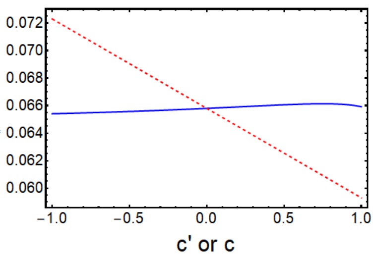
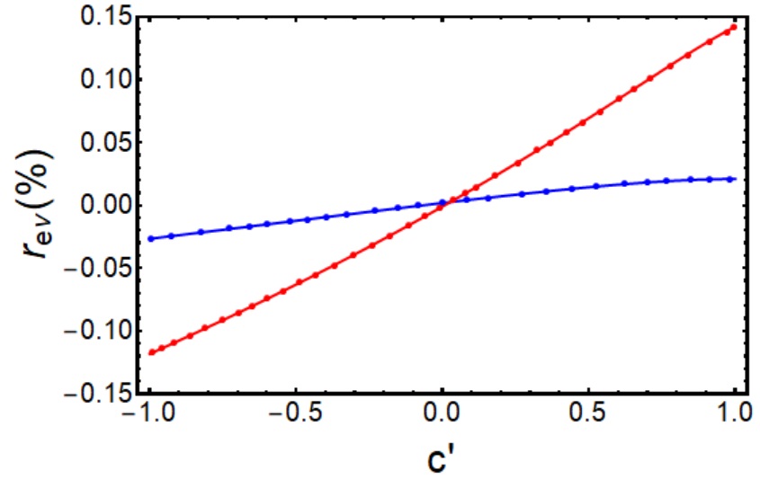
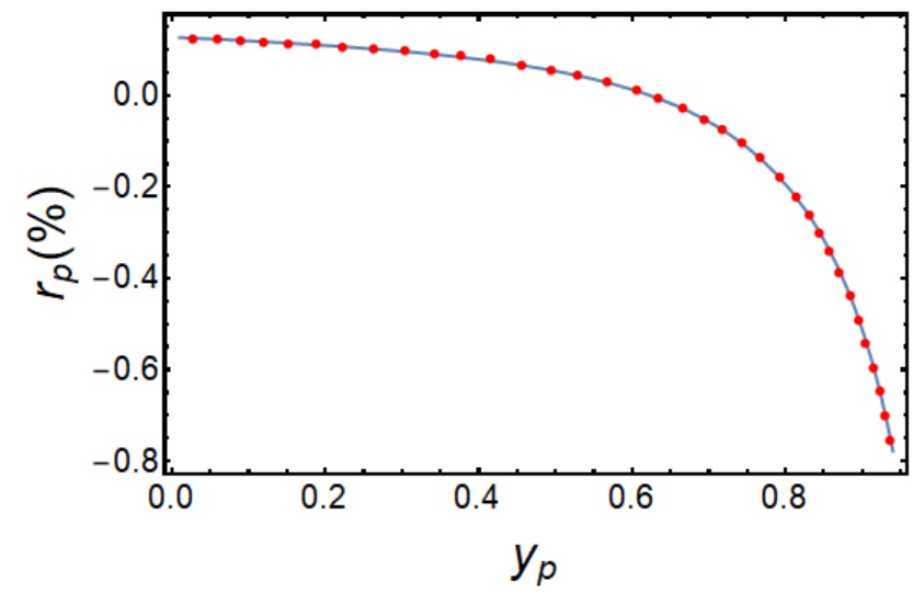
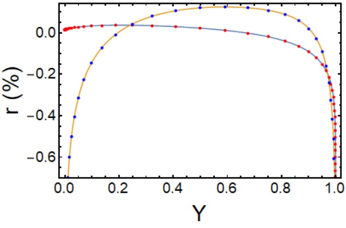
I argued before that, a mis-identification of p^ν\hat{p}_{\nu} by p^ν\hat{p}_{\nu}^{\prime} in the ν\nu-formalism would lead to an error of the order α/π103\alpha/\pi\sim 10^{-3}. To see this, let us compare the numerical results deduced from Eqs.(43) and (45) for the case of neutron decay: ζ=1\zeta=-1, mi=mnm_{i}=m_{n}, mf=mpm_{f}=m_{p}. I start from the spin-independent part of the outer RC, namely (α/2π)δtot0(\alpha/2\pi)\delta_{\text{tot}}^{0} in the ν\nu^{\prime}-formalism and (α/2π)[(1+3λ2)δ1+(1λ2)(δ1+δ2)βc](\alpha/2\pi)[(1+3\lambda^{2})\delta_{1}+(1-\lambda^{2})(\delta_{1}+\delta_{2})\beta c] in the ν\nu-formalism; they affect the precise extraction of the neutrino-electron correlation coefficient aa. From the first diagram in Fig.2 one sees that the dependence of these functions on their respective cosines indeed shows a difference at the order 10310^{-3}. Also, to compare with existing literature, in the second diagram I plot the the {Ee,c}\{E_{e},c^{\prime}\} Dalitz distribution of the outer RC:

reν(Ee,c)δ(dΓ/dEedc)outer(dΓ/dEedc)treeδ(dΓ/dEe)outer(dΓ/dEe)treeα2π[δtot0(Ee,c,λ)1+3λ2+(1λ2)βcδ1(Ee)]r_{e\nu}(E_{e},c^{\prime})\equiv\frac{\delta(d\Gamma/dE_{e}dc^{\prime})_{\text{outer}}}{(d\Gamma/dE_{e}dc^{\prime})_{\text{tree}}}-\frac{\delta(d\Gamma/dE_{e})_{\text{outer}}}{(d\Gamma/dE_{e})_{\text{tree}}}\approx\frac{\alpha}{2\pi}\left[\frac{\delta_{\text{tot}}^{0}(E_{e},c^{\prime},\lambda)}{1+3\lambda^{2}+(1-\lambda^{2})\beta c^{\prime}}-\delta_{1}(E_{e})\right] (48)

at two different EeE_{e}; one finds excellent agreement with Fig.8 of Ref.[23]. One also notices that a table of reν(Ee,c)r_{e\nu}(E_{e},c^{\prime}) was given in an earlier paper [16], but using my analytic expressions one finds that some entries in that table are off by an absolute value of 0.01%\sim 0.01\%. My new results are displayed in Table 1, but for practical applications one should of course recompute everything using my given formula instead of just applying the table.

Refer to caption
Figure 3: The difference (α/2π)[δ¯ν(Ee,λ)2λ(λ1)δ1(Ee)](\alpha/2\pi)[\bar{\delta}_{\nu}^{\prime}(E_{e},\lambda)-2\lambda(\lambda-1)\delta_{1}(E_{e})] as a function of EeE_{e}. Again I take λ=1.27\lambda=-1.27.

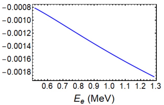
Next I study a more interesting quantity, namely the outer RC needed to extract the neutrino asymmetry parameter BB. At 𝒪(α0)\mathcal{O}(\alpha^{0}) (which does not distinguish ν\nu^{\prime} from ν\nu), a possible way to extract BB is to flip the neutron spin and integrate over Ωe\Omega_{e}:

(dΓdEedΩν())tree|s^()|s^Bs^p^ν().\left.\left(\frac{d\Gamma}{dE_{e}d\Omega_{\nu}^{(\prime)}}\right)_{\text{tree}}\right|_{\hat{s}}-\left.(\dots)\right|_{-\hat{s}}\propto B\hat{s}\cdot\hat{p}_{\nu}^{(\prime)}\leavevmode\nobreak\ . (49)

However, outer correction to the expression above takes very different forms in the ν\nu- and ν\nu^{\prime}-formalism:

δ(dΓdEedΩν)outer|s^()|s^\displaystyle\delta\left.\left(\frac{d\Gamma}{dE_{e}d\Omega_{\nu}}\right)_{\text{outer}}\right|_{\hat{s}}-\left.(\dots)\right|_{-\hat{s}} \displaystyle\propto α2π×2λ(λ1)δ1(Ee)s^p^ν\displaystyle\frac{\alpha}{2\pi}\times 2\lambda(\lambda-1)\delta_{1}(E_{e})\hat{s}\cdot\hat{p}_{\nu}
δ(dΓdEedΩν)outer|s^()|s^\displaystyle\delta\left.\left(\frac{d\Gamma}{dE_{e}d\Omega_{\nu}^{\prime}}\right)_{\text{outer}}\right|_{\hat{s}}-\left.(\dots)\right|_{-\hat{s}} \displaystyle\propto α2π×121+1𝑑c[δtotν(Ee,c,λ)+βcδtotβ(Ee,c,λ)]s^p^ν\displaystyle\frac{\alpha}{2\pi}\times\frac{1}{2}\int_{-1}^{+1}dc^{\prime}\left[\delta_{\text{tot}}^{\nu}(E_{e},c^{\prime},\lambda)+\beta c^{\prime}\delta_{\text{tot}}^{\beta}(E_{e},c^{\prime},\lambda)\right]\hat{s}\cdot\hat{p}_{\nu}^{\prime} (50)
\displaystyle\equiv α2πδ¯ν(Ee,λ)s^p^ν\displaystyle\frac{\alpha}{2\pi}\bar{\delta}_{\nu}^{\prime}(E_{e},\lambda)\hat{s}\cdot\hat{p}_{\nu}^{\prime}

One sees that, unlike the ν\nu-formalism that probes only the s^p^ν\hat{s}\cdot\hat{p}_{\nu} term in the outer correction, the ν\nu^{\prime}-formalism probes both the s^p^ν\hat{s}\cdot\hat{p}_{\nu}^{\prime} and s^β\hat{s}\cdot\vec{\beta} terms, because both their coefficients are functions of cc^{\prime}. In Fig.3 I plot the difference between the function (α/2π)δ¯ν(Ee,λ)(\alpha/2\pi)\bar{\delta}_{\nu}^{\prime}(E_{e},\lambda) (defined above) and (α/2π)×2λ(λ1)δ1(Ee)(\alpha/2\pi)\times 2\lambda(\lambda-1)\delta_{1}(E_{e}), and see that it is again of the order 10310^{-3}. This means, a mis-identification of p^ν\hat{p}_{\nu} by p^ν\hat{p}_{\nu}^{\prime} in the ν\nu-formalism would lead to a 10310^{-3} error in the extraction of BB.

V Radiative corrections in the recoil formalism

In some experiments such as aCORN and Nab [36], it is EfE_{f} instead of Ων\Omega_{\nu}^{\prime} that is being measured; in this case the recoil formalism, and not ν\nu^{\prime}, is the more appropriate description for the outer RC. So, for the sake of completeness I provide also the set of analytic expressions to compute the outer RC of the differential decay rate in the recoil formalism, in full analogy to those in the ν\nu^{\prime}-formalism from the previous sections.

First, it is obvious that one has no access to spin-dependent correlations if only EeE_{e} and EfE_{f} are measured, because there would be no vector to contract with s^\hat{s} as all solid angles of momenta are integrated out. Thus, for decays of polarized nuclei it is more natural to adopt the ν\nu^{\prime}-formalism where the solid angles Ωe\Omega_{e} and Ων\Omega_{\nu}^{\prime} are fixed, whereas in the recoil formalism I shall restrict myself to unpolarized nuclei. I start with the tree-level squared amplitude in the non-recoil limit, Eq.(29), and recast the variables in terms of 4-vector products:

Ee=pipemi,Eν=pipνmi,pepν=pipepipνmi2pepν,E_{e}=\frac{p_{i}\cdot p_{e}}{m_{i}}\leavevmode\nobreak\ ,\leavevmode\nobreak\ E_{\nu}^{\prime}=\frac{p_{i}\cdot p_{\nu}^{\prime}}{m_{i}}\leavevmode\nobreak\ ,\leavevmode\nobreak\ \vec{p}_{e}\cdot\vec{p}_{\nu}^{\prime}=\frac{p_{i}\cdot p_{e}p_{i}\cdot p_{\nu}^{\prime}}{m_{i}^{2}}-p_{e}\cdot p_{\nu}^{\prime}\leavevmode\nobreak\ , (51)

which allows to express the squared amplitude as a function of {y,z}\{y,z\} (recall that x=0x=0 for 3-body decay). That gives the tree-level differential rate:

(dΓdydz)tree𝒟3GV2m5(4π)3{(1+3λ2)y(2yz)+(1λ2)[y(2yz)+2(rerf+z1)]},\left(\frac{d\Gamma}{dydz}\right)_{\text{tree}}^{\mathcal{D}_{3}}\approx\frac{G_{V}^{2}m^{5}}{(4\pi)^{3}}\left\{(1+3\lambda^{2})y(2-y-z)+(1-\lambda^{2})\left[y(2-y-z)+2(r_{e}-r_{f}+z-1)\right]\right\}\leavevmode\nobreak\ , (52)

where the superscript 𝒟3\mathcal{D}_{3} denotes that the expression survives only if {y,z}𝒟3\{y,z\}\in\mathcal{D}_{3}.

The determination of the outer RC proceeds in the exact same way as before: For the virtual corrections, I take again the results in Refs.[7, 8, 9] and use Eq.(51) to recast them in terms of {y,z}\{y,z\}; this contribution survives only in the 𝒟3\mathcal{D}_{3} region. For the bremsstrahlung contribution, I follow Sec.IV.1 and split the squared amplitude into two pieces:

||2=|I|a2+||reg2,|\mathcal{M}|^{2}=|\mathcal{M}_{\text{I}}|_{a}^{2}+|\mathcal{M}|_{\text{reg}}^{2}\leavevmode\nobreak\ , (53)

and plug it into Eq.(19); the xx-integral is evaluated analytically for |I|a2|\mathcal{M}_{\text{I}}|^{2}_{a} and numerically for ||reg2|\mathcal{M}|^{2}_{\text{reg}}. The IR-divergence occurs in the xx-integral of |I|a2|\mathcal{M}_{\text{I}}|_{a}^{2} in the 𝒟3\mathcal{D}_{3} region, which analytic result can be found in Appendix D of Ref.[30]; it combines with the virtual correction to yield an IR-finite outcome. Meanwhile, for the “regular” piece I expand the squared amplitude as:

||reg2=4GV2αm2ij1(pk)i(pek)jdij,|\mathcal{M}|_{\text{reg}}^{2}=4G_{V}^{2}\alpha m^{2}\sum_{ij}\frac{1}{(p\cdot k)^{i}(p_{e}\cdot k)^{j}}d_{ij}\leavevmode\nobreak\ , (54)

where the expansion coefficients are just dij=2EeEν2Cij0d_{ij}=2E_{e}E_{\nu}^{\prime 2}C_{ij}^{0}; nevertheless, I still provide their analytic expressions in terms of {x,y,z}\{x,y,z\} in Appendix F for the convenience of readers. The pνp_{\nu}- and kk-integrals can be performed analytically using Appendix C.

Combining all the above, I obtain the total outer RC in the 𝒟3\mathcal{D}_{3} and 𝒟43\mathcal{D}_{4-3} region as follows:

δ(dΓdydz)outer𝒟3\displaystyle\delta\left(\frac{d\Gamma}{dydz}\right)_{\text{outer}}^{\mathcal{D}_{3}} =\displaystyle= GV2m5(4π)3α2π{(1+3λ2)y(2yz)δanr+2(1λ2)α+δIa2r\displaystyle\frac{G_{V}^{2}m^{5}}{(4\pi)^{3}}\frac{\alpha}{2\pi}\left\{(1+3\lambda^{2})y(2-y-z)\delta_{\text{an}}^{r}+2(1-\lambda^{2})\alpha_{+}\delta_{\text{Ia2}}^{r}\right.
+(1λ2)[y(2yz)+2(rerf+z1)](δanr+δv2)+δregr,𝒟3}\displaystyle\left.+(1-\lambda^{2})\left[y(2-y-z)+2(r_{e}-r_{f}+z-1)\right](\delta_{\text{an}}^{r}+\delta_{v2})+\delta_{\text{reg}}^{r,\mathcal{D}_{3}}\right\}
δ(dΓdydz)outer𝒟43\displaystyle\delta\left(\frac{d\Gamma}{dydz}\right)_{\text{outer}}^{\mathcal{D}_{4-3}} =\displaystyle= GV2m5(4π)3α2π{δIa2rlnα+α[(1+3λ2)y(2yz)+(1λ2)(y(2yz)\displaystyle\frac{G_{V}^{2}m^{5}}{(4\pi)^{3}}\frac{\alpha}{2\pi}\left\{\delta_{\text{Ia2}}^{r}\ln\frac{\alpha_{+}}{\alpha_{-}}\left[(1+3\lambda^{2})y(2-y-z)+(1-\lambda^{2})\left(y(2-y-z)\right.\right.\right. (55)
+2(rerf+z1))]+2(1λ2)(α+α)δIa2r+δregr,𝒟43},\displaystyle\left.\left.\left.+2(r_{e}-r_{f}+z-1)\right)\right]+2(1-\lambda^{2})(\alpha_{+}-\alpha_{-})\delta_{\text{Ia2}}^{r}+\delta_{\text{reg}}^{r,\mathcal{D}_{4-3}}\right\}\leavevmode\nobreak\ ,

where the functions at the right hand side are (the extra superscript rr stands for “recoil”):

δanr(y,z)\displaystyle\delta_{\text{an}}^{r}(y,z) =\displaystyle= (2βtanh1β+12)lnm2me2114+(2βtanh1β1)lnm2α+24P02\displaystyle\left(\frac{2}{\beta}\tanh^{-1}\beta+\frac{1}{2}\right)\ln\frac{m^{2}}{m_{e}^{2}}-\frac{11}{4}+\left(\frac{2}{\beta}\tanh^{-1}\beta-1\right)\ln\frac{m^{2}\alpha_{+}^{2}}{4P_{0}^{2}}
+ln(rerf+z1)2α+21βLi2(2β1+β)1βLi2(2β1β)\displaystyle+\ln\frac{(r_{e}-r_{f}+z-1)^{2}}{\alpha_{+}^{2}}-\frac{1}{\beta}\text{Li}_{2}\left(\frac{2\beta}{1+\beta}\right)-\frac{1}{\beta}\text{Li}_{2}\left(-\frac{2\beta}{1-\beta}\right)
2βLi2(β1+β(P1P0+1))+2βLi2(β1β(P1P01))\displaystyle-\frac{2}{\beta}\text{Li}_{2}\left(\frac{\beta}{1+\beta}\left(\frac{P_{1}}{P_{0}}+1\right)\right)+\frac{2}{\beta}\text{Li}_{2}\left(\frac{\beta}{1-\beta}\left(\frac{P_{1}}{P_{0}}-1\right)\right)
2β(tanh1β)2+2βtanh1β\displaystyle-\frac{2}{\beta}\left(\tanh^{-1}\beta\right)^{2}+2\beta\tanh^{-1}\beta
δIa2r(y)\displaystyle\delta_{\text{Ia2}}^{r}(y) =\displaystyle= 4(1βtanh1β1)\displaystyle 4\left(\frac{1}{\beta}\tanh^{-1}\beta-1\right)
δv2(y)\displaystyle\delta_{v2}(y) =\displaystyle= 2(1β2)βtanh1β\displaystyle\frac{2(1-\beta^{2})}{\beta}\tanh^{-1}\beta
δregr,𝒟3(y,z)\displaystyle\delta_{\text{reg}}^{r,\mathcal{D}_{3}}(y,z) =\displaystyle= ij0α+𝑑xdijIi,j\displaystyle\sum_{ij}\int_{0}^{\alpha_{+}}dxd_{ij}I_{i,j}
δregr,𝒟43(y,z)\displaystyle\delta_{\text{reg}}^{r,\mathcal{D}_{4-3}}(y,z) =\displaystyle= ijαα+𝑑xdijIi,j,\displaystyle\sum_{ij}\int_{\alpha_{-}}^{\alpha_{+}}dxd_{ij}I_{i,j}\leavevmode\nobreak\ , (56)

with

P0=m2(2yz),P1=m2βy[y(2yz)+2(rerf+z1)],P_{0}=\frac{m}{2}(2-y-z)\leavevmode\nobreak\ ,\leavevmode\nobreak\ P_{1}=\frac{m}{2\beta y}\left[y(2-y-z)+2(r_{e}-r_{f}+z-1)\right]\leavevmode\nobreak\ , (57)

and the electron speed β=y24re/y\beta=\sqrt{y^{2}-4r_{e}}/y.

Refer to caption
Refer to caption
Figure 4: Left: The function rpr_{p} with respect to the proton kinetic energy T=ypTmax=yp((mnmp)2me2)/(2mn)T=y_{p}T_{\text{max}}=y_{p}((m_{n}-m_{p})^{2}-m_{e}^{2})/(2m_{n}), with λ=1.27\lambda=-1.27; solid line is my result and dots are discrete points extracted from Fig.7 in Ref.[23]. Right: My predictions of the function rr at X=0.2X=0.2 (blue solid line) and X=0.8X=0.8 (yellow solid line); dots are corresponding discrete points extracted from Fig.6(a) in Ref.[23].

Eq.(55) is the third central result of this work; a simple consistency check is that it must reproduce the same outer RC to the beta spectrum as in Sirlin’s approach, up to small recoil corrections (on top of the RC). This implies:

δ(dΓ/dy)outer(dΓ/dy)tree=𝑑zδ(dΓ/dydz)outer𝑑z(dΓ/dydz)treeα2πδ1(Ee), 2re<y<1+rerf.\frac{\delta\left(d\Gamma/dy\right)_{\text{outer}}}{\left(d\Gamma/dy\right)_{\text{tree}}}=\frac{\int dz\delta\left(d\Gamma/dydz\right)_{\text{outer}}}{\int dz\left(d\Gamma/dydz\right)_{\text{tree}}}\approx\frac{\alpha}{2\pi}\delta_{1}(E_{e})\leavevmode\nobreak\ ,\leavevmode\nobreak\ 2\sqrt{r_{e}}<y<1+r_{e}-r_{f}\leavevmode\nobreak\ . (58)

Substituting the neutron decay parameters, one finds that this relation is satisfied to a <0.1%<0.1\% relative error, which proves the correctness of all the analytic formula. To provide further cross-check, I compute two more functions: The first is the relative RC rpr_{p} to the proton spectrum in neutron decay defined in Ref.[23], which reads:

rp(T)δ(dΓ/dz)outer(dΓ/dz)treeδΓouterΓtree,r_{p}(T)\equiv\frac{\delta\left(d\Gamma/dz\right)_{\text{outer}}}{\left(d\Gamma/dz\right)_{\text{tree}}}-\frac{\delta\Gamma_{\text{outer}}}{\Gamma_{\text{tree}}}\leavevmode\nobreak\ , (59)

where I use the proton kinetic energy T=mnz/2mpT=m_{n}z/2-m_{p} as the variable. The second is the relative RC of the Dalitz distribution {y,z}\{y,z\} in the 𝒟3\mathcal{D}_{3} region as defined in the same reference:

r(y,z)δ(dΓ/dydz)outer𝒟3(dΓ/dydz)treeδ(dΓ/dy)outer𝒟3(dΓ/dy)tree,r(y,z)\equiv\frac{\delta(d\Gamma/dydz)_{\text{outer}}^{\mathcal{D}_{3}}}{(d\Gamma/dydz)_{\text{tree}}}-\frac{\delta(d\Gamma/dy)_{\text{outer}}^{\mathcal{D}_{3}}}{(d\Gamma/dy)_{\text{tree}}}\leavevmode\nobreak\ , (60)

where the results are expressed in terms of two new variables {X,Y}\{X,Y\} (which correspond to {x,y}\{x,y\} in Ref.[23]), defined through:

y=2mn(me+(Emme)X),z=zmin+(zmaxzmin)Y,y=\frac{2}{m_{n}}(m_{e}+(E_{m}-m_{e})X)\leavevmode\nobreak\ ,\leavevmode\nobreak\ z=z_{\text{min}}+(z_{\text{max}}-z_{\text{min}})Y\leavevmode\nobreak\ , (61)

with zmin=a(y)b(y)z_{\text{min}}=a(y)-b(y), zmax=a(y)+b(y)z_{\text{max}}=a(y)+b(y) in the 𝒟3\mathcal{D}_{3} region. The outcomes are plotted in Fig.4 and one again observes excellent agreement with the results in Ref.[23] obtained using numerical packages.

VI Summary

In this paper I carefully analyze the theory structure of the so-called ν\nu^{\prime}-formalism, which is designed to bypass the conceptual problem in the traditional treatment of outer RC by Sirlin, Shann and Garcia-Maya. The formalism itself has already appeared in many literature and is not at all a new concept, but this paper provides the most elegant representation of the 4-body phase space formula consistent to the non-recoil approximation. With this master formula, I derive the full set of analytic expressions needed for the evaluation of the outer RC to the differential rate of a Ji=Jf=1/2J_{i}=J_{f}=1/2 (or 0) nuclear β±\beta^{\pm} decay. The results are explicitly mγm_{\gamma}-independent, and require only a minimal amount of numerical integration. I compare the outcome with existing literature and discuss its implications on pν\vec{p}_{\nu}^{\prime}-dependent observables. Similar analytic expressions in the recoil formalism are also derived assuming unpolarized nuclei.

While the master formula for the 4-body phase space is completely general, I restrict myself to spin-half systems which allows us to make use of the elegant spinor technique in field theory that simplifies the squared amplitude. Generalization to generic nuclear beta decays with arbitrary Ji,fJ_{i,f} may involve, apart from more complicated analytic expressions for existing terms, new spin-dependent correlation structures such as the cc-coefficient [4]. Its outer RC may be studied either using traditional approaches focusing on the “convention term” contribution [37], or using the more recent effective field theory description [38, 39, 40]. This will be worked out in a follow-up work.

Acknowledgements.
I thank Ferenc Glück for many useful discussions and for cross-checking my results. I was supported in part by the U.S. Department of Energy (DOE), Office of Science, Office of Nuclear Physics, under the FRIB Theory Alliance award DE-SC0013617, and by the DOE grant DE-FG02-97ER41014. I acknowledge support from the DOE Topical Collaboration “Nuclear Theory for New Physics”, award No. DE-SC0023663.

Appendix A IR-divergent phase space integral

In the ν\nu^{\prime}-formalism, the only IR-divergent phase space integral reads:

0Eνd|pν||pν|2d3k(2π)32Ekd3pν(2π)32Eν(2π)4δ(4)(pνpνk)(ppkpepek)2Eν8πδIa1.\int_{0}^{E_{\nu}^{\prime}}d|\vec{p}_{\nu}^{\prime}||\vec{p}_{\nu}^{\prime}|^{2}\int\frac{d^{3}k}{(2\pi)^{3}2E_{k}}\frac{d^{3}p_{\nu}}{(2\pi)^{3}2E_{\nu}}(2\pi)^{4}\delta^{(4)}(p_{\nu}^{\prime}-p_{\nu}-k)\left(\frac{p}{p\cdot k}-\frac{p_{e}}{p_{e}\cdot k}\right)^{2}\equiv-\frac{E_{\nu}^{\prime}}{8\pi}\delta_{\text{I}a1}\leavevmode\nobreak\ . (62)

The IR-divergence arises from the |pν||\vec{p}_{\nu}^{\prime}|-integral at |pν|Eν|\vec{p}_{\nu}^{\prime}|\rightarrow E_{\nu}^{\prime}. One may evaluate this integral using the method outlined in Ref.[30], namely to apply dimensional regularization of the photon momentum [41]:

d3k(2π)32Ekμ4ddd1k(2π)d12Ek.\frac{d^{3}k}{(2\pi)^{3}2E_{k}}\rightarrow\mu^{4-d}\frac{d^{d-1}k}{(2\pi)^{d-1}2E_{k}}\leavevmode\nobreak\ . (63)

A important advantage of this method is that the massless on-shell condition k2=0k^{2}=0 still holds, which greatly simplifies the intermediate steps. After finishing the evaluation, one may choose to switch back to the photon-mass prescription by the following matching:

24dγE+ln4πlnmγ2μ2.\frac{2}{4-d}-\gamma_{E}+\ln 4\pi\rightarrow\ln\frac{m_{\gamma}^{2}}{\mu^{2}}\leavevmode\nobreak\ . (64)

With this, I obtain the result of the integral as:

δIa1(Ee,c)\displaystyle\delta_{\text{I}a1}(E_{e},c^{\prime}) =\displaystyle= 2(4ln4Eν2mγ2)(1βtanh1β1)+2tanh1β+2ln(1βc1+β)\displaystyle-2\left(4-\ln\frac{4E_{\nu}^{\prime 2}}{m_{\gamma}^{2}}\right)\left(\frac{1}{\beta}\tanh^{-1}\beta-1\right)+2\tanh^{-1}\beta+2\ln\left(\frac{1-\beta c^{\prime}}{1+\beta}\right) (65)
+1βLi2(2β1+β)1βLi2(2β1β)2βLi2(β(c+1)1+β)\displaystyle+\frac{1}{\beta}\text{Li}_{2}\left(\frac{2\beta}{1+\beta}\right)-\frac{1}{\beta}\text{Li}_{2}\left(\frac{-2\beta}{1-\beta}\right)-\frac{2}{\beta}\text{Li}_{2}\left(\frac{\beta(c^{\prime}+1)}{1+\beta}\right)
+2βLi2(β(c1)1β).\displaystyle+\frac{2}{\beta}\text{Li}_{2}\left(\frac{\beta(c^{\prime}-1)}{1-\beta}\right)\leavevmode\nobreak\ .

For terms proportional to p^ν\hat{p}_{\nu}^{\prime} in |I|a2|\mathcal{M}_{\text{I}}|^{2}_{a}, the involved integral is Eq.(62) but with an extra factor 1+(|pν|Eν)/Eν1+(|\vec{p}_{\nu}^{\prime}|-E_{\nu}^{\prime})/E_{\nu}^{\prime} multiplied to the integrand. The integration returns (Eν/8π)(δIa1+δIa2)-(E_{\nu}^{\prime}/8\pi)(\delta_{\text{I}a1}+\delta_{\text{I}a2}), where

δIa2(Ee)=4(1ln4)(1βtanh1β1).\delta_{\text{I}a2}(E_{e})=4(1-\ln 4)\left(\frac{1}{\beta}\tanh^{-1}\beta-1\right)\leavevmode\nobreak\ . (66)

Appendix B Virtual outer corrections

Refer to caption
Figure 5: Self-energy and one-particle irreducible diagrams that contribute to the outer RC.

The SM one-loop RC to beta decay contribute to three quantities: (1) The Fermi function [6] that describes the Coulomb interaction between the outgoing electron and the daughter nucleus; (2) The “outer” RC that summarizes all the non-Fermi and EeE_{e}-dependent corrections; (3) The “inner” RC which only effect is to renormalize the effective weak coupling constants. In this paper I am only interested in the outer RC, which is obtained by computing the Feynman diagrams in Fig.5, taking the nuclei as point-like particles. For a Ji=Jf=1/2J_{i}=J_{f}=1/2 decay with polarized parent nucleus, the outcome in the non-recoil limit reads [7, 8, 9]:

δ(dΓdEedΩedΩν)v\displaystyle\delta\left(\frac{d\Gamma}{dE_{e}d\Omega_{e}d\Omega_{\nu}^{\prime}}\right)_{v} =\displaystyle= GV2(2π)5|pe|EeEν2α2π{(1+3λ2)δv1+(1λ2)(δv1+δv2)βp^ν\displaystyle\frac{G_{V}^{2}}{(2\pi)^{5}}|\vec{p}_{e}|E_{e}E_{\nu}^{\prime 2}\frac{\alpha}{2\pi}\left\{(1+3\lambda^{2})\delta_{v1}+(1-\lambda^{2})(\delta_{v1}+\delta_{v2})\vec{\beta}\cdot\hat{p}_{\nu}^{\prime}\right. (67)
+s^[2λ(λζ1)(δv1+δv2)β2λ(λζ+1)δv1p^ν]},\displaystyle\left.+\hat{s}\cdot\left[2\lambda(\lambda\zeta-1)(\delta_{v1}+\delta_{v2})\vec{\beta}-2\lambda(\lambda\zeta+1)\delta_{v1}\hat{p}_{\nu}^{\prime}\right]\right\}\leavevmode\nobreak\ ,

where

δv1(Ee)\displaystyle\delta_{v1}(E_{e}) =\displaystyle= 2lnme2mγ2(1βtanh1β1)+32lnm2me21142βLi2(2β1+β)\displaystyle-2\ln\frac{m_{e}^{2}}{m_{\gamma}^{2}}\left(\frac{1}{\beta}\tanh^{-1}\beta-1\right)+\frac{3}{2}\ln\frac{m^{2}}{m_{e}^{2}}-\frac{11}{4}-\frac{2}{\beta}\text{Li}_{2}\left(\frac{2\beta}{1+\beta}\right)
2β(tanh1β)2+2βtanh1β\displaystyle-\frac{2}{\beta}(\tanh^{-1}\beta)^{2}+2\beta\tanh^{-1}\beta
δv2(Ee)\displaystyle\delta_{v2}(E_{e}) =\displaystyle= 2(1β2)βtanh1β.\displaystyle\frac{2(1-\beta^{2})}{\beta}\tanh^{-1}\beta\leavevmode\nobreak\ . (68)

Appendix C Analytic formula for pνp_{\nu}- and kk-integration

If one drops the parent’s spin vector sμs^{\mu}, then there are only three vectors that can be dotted to the photon momentum kk in the squared amplitude: pp, pep_{e} and pνp_{\nu}^{\prime}; but momentum conservation pνk=pνp_{\nu}^{\prime}-k=p_{\nu} implies 2pνk=pν22p_{\nu}^{\prime}\cdot k=p_{\nu}^{\prime 2} assuming massless neutrino. The pνp_{\nu}- and kk-integrations in ||reg2|\mathcal{M}|^{2}_{\text{reg}} can be represented in terms of the functions below:

Ii,j(Ee,c,|pν|)d3k(2π)32Ekd3pν(2π)32Eν(2π)4δ(4)(pνpνk)1(pk)i(pek)j,I_{i,j}(E_{e},c^{\prime},|\vec{p}_{\nu}^{\prime}|)\equiv\int\frac{d^{3}k}{(2\pi)^{3}2E_{k}}\frac{d^{3}p_{\nu}}{(2\pi)^{3}2E_{\nu}}(2\pi)^{4}\delta^{(4)}(p_{\nu}^{\prime}-p_{\nu}-k)\frac{1}{(p\cdot k)^{i}(p_{e}\cdot k)^{j}}\leavevmode\nobreak\ , (69)

where i,ji,j are integers. Analytic expressions of the functions needed in this work can be found in Ref.[13] (but beware of the difference in the overall normalization):

I0,0\displaystyle I_{0,0} =\displaystyle= 18π\displaystyle\frac{1}{8\pi}
I1,0\displaystyle I_{-1,0} =\displaystyle= αp16π\displaystyle\frac{\alpha_{p}}{16\pi}
I1,0\displaystyle I_{1,0} =\displaystyle= 18πβplnαp+βpαpβp\displaystyle\frac{1}{8\pi\beta_{p}}\ln\frac{\alpha_{p}+\beta_{p}}{\alpha_{p}-\beta_{p}}
I0,1\displaystyle I_{0,1} =\displaystyle= 18πβelnαe+βeαeβe\displaystyle\frac{1}{8\pi\beta_{e}}\ln\frac{\alpha_{e}+\beta_{e}}{\alpha_{e}-\beta_{e}}
I2,0\displaystyle I_{2,0} =\displaystyle= 12πm2pν2\displaystyle\frac{1}{2\pi m^{2}p_{\nu}^{\prime 2}}
I0,2\displaystyle I_{0,2} =\displaystyle= 12πme2pν2\displaystyle\frac{1}{2\pi m_{e}^{2}p_{\nu}^{\prime 2}}
I1,1\displaystyle I_{1,1} =\displaystyle= 14πγpepν2lnppe+γpeppeγpe\displaystyle\frac{1}{4\pi\gamma_{pe}p_{\nu}^{\prime 2}}\ln\frac{p\cdot p_{e}+\gamma_{pe}}{p\cdot p_{e}-\gamma_{pe}}
I1,1\displaystyle I_{1,-1} =\displaystyle= 18π((ppe:pν)βp2+pν2(pepν:p)2βp3lnαp+βpαpβp)\displaystyle\frac{1}{8\pi}\left(\frac{(pp_{e}:p_{\nu}^{\prime})}{\beta_{p}^{2}}+\frac{p_{\nu}^{\prime 2}(p_{e}p_{\nu}^{\prime}:p)}{2\beta_{p}^{3}}\ln\frac{\alpha_{p}+\beta_{p}}{\alpha_{p}-\beta_{p}}\right)
I1,1\displaystyle I_{-1,1} =\displaystyle= 18π((pep:pν)βe2+pν2(ppν:pe)2βe3lnαe+βeαeβe)\displaystyle\frac{1}{8\pi}\left(\frac{(p_{e}p:p_{\nu}^{\prime})}{\beta_{e}^{2}}+\frac{p_{\nu}^{\prime 2}(pp_{\nu}^{\prime}:p_{e})}{2\beta_{e}^{3}}\ln\frac{\alpha_{e}+\beta_{e}}{\alpha_{e}-\beta_{e}}\right)
I2,1\displaystyle I_{2,-1} =\displaystyle= 18π(2(pepν:p)m2βp2+(ppe:pν)βp3lnαp+βpαpβp)\displaystyle\frac{1}{8\pi}\left(\frac{2(p_{e}p_{\nu}^{\prime}:p)}{m^{2}\beta_{p}^{2}}+\frac{(pp_{e}:p_{\nu}^{\prime})}{\beta_{p}^{3}}\ln\frac{\alpha_{p}+\beta_{p}}{\alpha_{p}-\beta_{p}}\right)
I1,2\displaystyle I_{-1,2} =\displaystyle= 18π(2(ppν:pe)me2βe2+(pep:pν)βe3lnαe+βeαeβe)\displaystyle\frac{1}{8\pi}\left(\frac{2(pp_{\nu}^{\prime}:p_{e})}{m_{e}^{2}\beta_{e}^{2}}+\frac{(p_{e}p:p_{\nu}^{\prime})}{\beta_{e}^{3}}\ln\frac{\alpha_{e}+\beta_{e}}{\alpha_{e}-\beta_{e}}\right)
I2,1\displaystyle I_{-2,1} =\displaystyle= 18π[(pν2)2(ppν:pe)24βe5lnαe+βeαeβe+pν2(pep:pν)(ppν:pe)βe4+αe(pep:pν)22βe4\displaystyle\frac{1}{8\pi}\left[\frac{(p_{\nu}^{\prime 2})^{2}(pp_{\nu}^{\prime}:p_{e})^{2}}{4\beta_{e}^{5}}\ln\frac{\alpha_{e}+\beta_{e}}{\alpha_{e}-\beta_{e}}+\frac{p_{\nu}^{\prime 2}(p_{e}p:p_{\nu}^{\prime})(pp_{\nu}^{\prime}:p_{e})}{\beta_{e}^{4}}+\frac{\alpha_{e}(p_{e}p:p_{\nu}^{\prime})^{2}}{2\beta_{e}^{4}}\right.
+(βe2βp2(pep:pν)24βe4)(αeme2pν22βelnαe+βeαeβe)]\displaystyle\left.+\left(\frac{\beta_{e}^{2}\beta_{p}^{2}-(p_{e}p:p_{\nu}^{\prime})^{2}}{4\beta_{e}^{4}}\right)\left(\alpha_{e}-\frac{m_{e}^{2}p_{\nu}^{\prime 2}}{2\beta_{e}}\ln\frac{\alpha_{e}+\beta_{e}}{\alpha_{e}-\beta_{e}}\right)\right]
I2,2\displaystyle I_{-2,2} =\displaystyle= 18π[pν2(ppν:pe)2me2βe4+pν2(ppν:pe)(pep:pν)βe5lnαe+βeαeβe+(pep:pν)2βe4\displaystyle\frac{1}{8\pi}\left[\frac{p_{\nu}^{\prime 2}(pp_{\nu}^{\prime}:p_{e})^{2}}{m_{e}^{2}\beta_{e}^{4}}+\frac{p_{\nu}^{\prime 2}(pp_{\nu}^{\prime}:p_{e})(p_{e}p:p_{\nu}^{\prime})}{\beta_{e}^{5}}\ln\frac{\alpha_{e}+\beta_{e}}{\alpha_{e}-\beta_{e}}+\frac{(p_{e}p:p_{\nu}^{\prime})^{2}}{\beta_{e}^{4}}\right. (70)
(βe2βp2(pep:pν)22βe4)(2αeβelnαe+βeαeβe)].\displaystyle\left.-\left(\frac{\beta_{e}^{2}\beta_{p}^{2}-(p_{e}p:p_{\nu}^{\prime})^{2}}{2\beta_{e}^{4}}\right)\left(2-\frac{\alpha_{e}}{\beta_{e}}\ln\frac{\alpha_{e}+\beta_{e}}{\alpha_{e}-\beta_{e}}\right)\right]\leavevmode\nobreak\ .

Here I have defined:

αpppν,αepepν,βpαp2m2pν2,βeαe2me2pν2,\displaystyle\alpha_{p}\equiv p\cdot p_{\nu}^{\prime}\leavevmode\nobreak\ ,\leavevmode\nobreak\ \alpha_{e}\equiv p_{e}\cdot p_{\nu}^{\prime}\leavevmode\nobreak\ ,\leavevmode\nobreak\ \beta_{p}\equiv\sqrt{\alpha_{p}^{2}-m^{2}p_{\nu}^{\prime 2}}\leavevmode\nobreak\ ,\leavevmode\nobreak\ \beta_{e}\equiv\sqrt{\alpha_{e}^{2}-m_{e}^{2}p_{\nu}^{\prime 2}}\leavevmode\nobreak\ ,
γpe(ppe)2m2me2,(ab:c)(ac)(bc)c2(ab).\displaystyle\gamma_{pe}\equiv\sqrt{(p\cdot p_{e})^{2}-m^{2}m_{e}^{2}}\leavevmode\nobreak\ ,\leavevmode\nobreak\ (ab:c)\equiv(a\cdot c)(b\cdot c)-c^{2}(a\cdot b)\leavevmode\nobreak\ . (71)

Finally, in the ν\nu^{\prime}-formalism I use the following representation of the dot products:

p2=m2,ppe=mEe,ppν=mEν,pe2=me2,pepν=EeEν|pe||pν|c,\displaystyle p^{2}=m^{2}\leavevmode\nobreak\ ,\leavevmode\nobreak\ p\cdot p_{e}=mE_{e}\leavevmode\nobreak\ ,\leavevmode\nobreak\ p\cdot p_{\nu}^{\prime}=mE_{\nu}^{\prime}\leavevmode\nobreak\ ,\leavevmode\nobreak\ p_{e}^{2}=m_{e}^{2}\leavevmode\nobreak\ ,\leavevmode\nobreak\ p_{e}\cdot p_{\nu}^{\prime}=E_{e}E_{\nu}^{\prime}-|\vec{p}_{e}||\vec{p}_{\nu}^{\prime}|c^{\prime}\leavevmode\nobreak\ ,
pν2=Eν2|pν|2,\displaystyle p_{\nu}^{\prime 2}=E_{\nu}^{\prime 2}-|\vec{p}_{\nu}^{\prime}|^{2}\leavevmode\nobreak\ , (72)

whereas, in the recoil formalism I use:

p2=m2,ppe=m2y2,ppν=m22(2yz),pe2=m2re,\displaystyle p^{2}=m^{2}\leavevmode\nobreak\ ,\leavevmode\nobreak\ p\cdot p_{e}=\frac{m^{2}y}{2}\leavevmode\nobreak\ ,\leavevmode\nobreak\ p\cdot p_{\nu}^{\prime}=\frac{m^{2}}{2}(2-y-z)\leavevmode\nobreak\ ,\leavevmode\nobreak\ p_{e}^{2}=m^{2}r_{e}\leavevmode\nobreak\ ,
pepν=m22(1+rfrexz),pν2=m2x.\displaystyle p_{e}\cdot p_{\nu}^{\prime}=\frac{m^{2}}{2}(1+r_{f}-r_{e}-x-z)\leavevmode\nobreak\ ,\leavevmode\nobreak\ p_{\nu}^{\prime 2}=m^{2}x\leavevmode\nobreak\ . (73)

Appendix D pνp_{\nu}- and kk-integral with the spin vector

In this work I allow the parent nucleus to be polarized. This introduces the spin vector sμs^{\mu} which can appear at most linearly in the squared amplitude. So, in doing the pνp_{\nu}- and kk-integrations, one may also encounter integrals of the form

d3k(2π)32Ekd3pν(2π)32Eν(2π)4δ(4)(pνpνk)sk(pk)i(pek)j\int\frac{d^{3}k}{(2\pi)^{3}2E_{k}}\frac{d^{3}p_{\nu}}{(2\pi)^{3}2E_{\nu}}(2\pi)^{4}\delta^{(4)}(p_{\nu}^{\prime}-p_{\nu}-k)\frac{s\cdot k}{(p\cdot k)^{i}(p_{e}\cdot k)^{j}} (74)

in addition to those in Appendix C. To evaluate it, I first parameterize:

Ii,jμd3k(2π)32Ekd3pν(2π)32Eν(2π)4δ(4)(pνpνk)kμ(pk)i(pek)j=c1pμ+c2peμ+c3pνμ,I_{i,j}^{\mu}\equiv\int\frac{d^{3}k}{(2\pi)^{3}2E_{k}}\frac{d^{3}p_{\nu}}{(2\pi)^{3}2E_{\nu}}(2\pi)^{4}\delta^{(4)}(p_{\nu}^{\prime}-p_{\nu}-k)\frac{k^{\mu}}{(p\cdot k)^{i}(p_{e}\cdot k)^{j}}=c_{1}p^{\mu}+c_{2}p_{e}^{\mu}+c_{3}p_{\nu}^{\prime\mu}\leavevmode\nobreak\ , (75)

and evaluate the coefficients c1,2,3c_{1,2,3}. Contracting Eq.(75) with pμp_{\mu}, peμp_{e\mu} and (pν)μ(p_{\nu}^{\prime})_{\mu} gives rise to the following matrix equation:

(c1c2c3)=M1(Ii1,jIi,j1pν22Ii,j),M=(mN2ppeppνppeme2pepνppνpepνpν2).\left(\begin{array}[]{c}c_{1}\\ c_{2}\\ c_{3}\end{array}\right)=M^{-1}\left(\begin{array}[]{c}I_{i-1,j}\\ I_{i,j-1}\\ \frac{p_{\nu}^{\prime 2}}{2}I_{i,j}\end{array}\right)\leavevmode\nobreak\ ,\leavevmode\nobreak\ M=\left(\begin{array}[]{ccc}m_{N}^{2}&p\cdot p_{e}&p\cdot p_{\nu}^{\prime}\\ p\cdot p_{e}&m_{e}^{2}&p_{e}\cdot p_{\nu}^{\prime}\\ p\cdot p_{\nu}^{\prime}&p_{e}\cdot p_{\nu}^{\prime}&p_{\nu}^{\prime 2}\end{array}\right)\leavevmode\nobreak\ . (76)

Plugging this back to Eq.(75) and contracting to sμs_{\mu} gives:

sμIi,jμ\displaystyle s_{\mu}I_{i,j}^{\mu} =\displaystyle= [(M1)21Ii1,j+(M1)22Ii,j1+pν22(M1)23Ii,j]spe\displaystyle\left[(M^{-1})_{21}I_{i-1,j}+(M^{-1})_{22}I_{i,j-1}+\frac{p_{\nu}^{\prime 2}}{2}(M^{-1})_{23}I_{i,j}\right]s\cdot p_{e} (77)
+[(M1)31Ii1,j+(M1)32Ii,j1+pν22(M1)33Ii,j]spν.\displaystyle+\left[(M^{-1})_{31}I_{i-1,j}+(M^{-1})_{32}I_{i,j-1}+\frac{p_{\nu}^{\prime 2}}{2}(M^{-1})_{33}I_{i,j}\right]s\cdot p_{\nu}^{\prime}\leavevmode\nobreak\ .

So, the new integral is expressible in terms of the old integrals Ii,jI_{i,j}. In fact, this result can be conveniently implemented by making the following replacement at the squared amplitude:

sk\displaystyle s\cdot k \displaystyle\rightarrow [(M1)21spe+(M1)31spν]pk+[(M1)22spe+(M1)32spν]pek\displaystyle\left[(M^{-1})_{21}s\cdot p_{e}+(M^{-1})_{31}s\cdot p_{\nu}^{\prime}\right]p\cdot k+\left[(M^{-1})_{22}s\cdot p_{e}+(M^{-1})_{32}s\cdot p_{\nu}^{\prime}\right]p_{e}\cdot k (78)
+[(M1)23spe+(M1)33spν]pν2/2.\displaystyle+\left[(M^{-1})_{23}s\cdot p_{e}+(M^{-1})_{33}s\cdot p_{\nu}^{\prime}\right]p_{\nu}^{\prime 2}/2\leavevmode\nobreak\ .

Appendix E The coefficients CijXC_{ij}^{X}

Here I provide the analytic expressions of the coefficients CijXC_{ij}^{X} defined in Eq.(40).

E.1 Cij0C_{ij}^{0}

The non-zero coefficients are:

C000\displaystyle C_{00}^{0} =\displaystyle= 16π(λ2+1)EeEν2\displaystyle\frac{16\pi(\lambda^{2}+1)}{E_{e}E_{\nu}^{\prime 2}}
C100\displaystyle C_{10}^{0} =\displaystyle= 8πm(4Ee(1+3λ2)Eν)EeEν2\displaystyle\frac{8\pi m(4E_{e}-(1+3\lambda^{2})E_{\nu}^{\prime})}{E_{e}E_{\nu}^{\prime 2}}
C010\displaystyle C_{01}^{0} =\displaystyle= 4πEeEν2[(λ21)(2|pe||pν|c+|pν|2Eν22me2)+8Ee2(λ2+1)2EeEν(5λ2+3)]\displaystyle-\frac{4\pi}{E_{e}E_{\nu}^{\prime 2}}\left[(\lambda^{2}-1)(2|\vec{p}_{e}||\vec{p}_{\nu}^{\prime}|c^{\prime}+|\vec{p}_{\nu}^{\prime}|^{2}-E_{\nu}^{\prime 2}-2m_{e}^{2})+8E_{e}^{2}(\lambda^{2}+1)-2E_{e}E_{\nu}^{\prime}(5\lambda^{2}+3)\right]
C020\displaystyle C_{02}^{0} =\displaystyle= 4π(λ21)me2(|pν|2Eν2)EeEν2\displaystyle\frac{4\pi(\lambda^{2}-1)m_{e}^{2}(|\vec{p}_{\nu}^{\prime}|^{2}-E_{\nu}^{\prime 2})}{E_{e}E_{\nu}^{\prime 2}}
C110\displaystyle C_{11}^{0} =\displaystyle= 4π(λ21)m(Eν2|pν|2)Eν2\displaystyle\frac{4\pi(\lambda^{2}-1)m(E_{\nu}^{\prime 2}-|\vec{p}_{\nu}^{\prime}|^{2})}{E_{\nu}^{\prime 2}}
C110\displaystyle C_{-11}^{0} =\displaystyle= 16π(λ2+1)(2EeEν)EeEν2m\displaystyle-\frac{16\pi(\lambda^{2}+1)(2E_{e}-E_{\nu}^{\prime})}{E_{e}E_{\nu}^{\prime 2}m}
C210\displaystyle C_{2-1}^{0} =\displaystyle= 8π(λ21)m2EeEν2\displaystyle\frac{8\pi(\lambda^{2}-1)m^{2}}{E_{e}E_{\nu}^{\prime 2}}
C120\displaystyle C_{-12}^{0} =\displaystyle= 16π(λ2+1)me2(EeEν)EeEν2m\displaystyle\frac{16\pi(\lambda^{2}+1)m_{e}^{2}(E_{e}-E_{\nu}^{\prime})}{E_{e}E_{\nu}^{\prime 2}m}
C210\displaystyle C_{-21}^{0} =\displaystyle= 16π(λ2+1)EeEν2m2\displaystyle-\frac{16\pi(\lambda^{2}+1)}{E_{e}E_{\nu}^{\prime 2}m^{2}}
C220\displaystyle C_{-22}^{0} =\displaystyle= 16π(λ2+1)me2EeEν2m2\displaystyle\frac{16\pi(\lambda^{2}+1)m_{e}^{2}}{E_{e}E_{\nu}^{\prime 2}m^{2}} (79)

It is worth noticing that Cij0C_{ij}^{0} is independent of ζ\zeta, i.e. they are the same for β±\beta^{\pm} decay. This is not the case for the spin-dependent coefficients CijβC_{ij}^{\beta} and CijνC_{ij}^{\nu}.

E.2 CijβC_{ij}^{\beta}

The non-zero coefficients are:

C00β\displaystyle C_{00}^{\beta} =\displaystyle= 16πλ[|pν|(2(λζ+2)Ee+(λζ+1)Eν)+|pe|cEν(λζ+1)]|pe|2|pν|(c21)Eν2\displaystyle-\frac{16\pi\lambda\left[|\vec{p}_{\nu}^{\prime}|(-2(\lambda\zeta+2)E_{e}+(-\lambda\zeta+1)E_{\nu}^{\prime})+|\vec{p}_{e}|c^{\prime}E_{\nu}^{\prime}(\lambda\zeta+1)\right]}{|\vec{p}_{e}|^{2}|\vec{p}_{\nu}^{\prime}|(c^{\prime 2}-1)E_{\nu}^{\prime 2}}
C10β\displaystyle C_{-10}^{\beta} =\displaystyle= 32πλ|pe|2(c21)Eν2m\displaystyle\frac{32\pi\lambda}{|\vec{p}_{e}|^{2}(c^{\prime 2}-1)E_{\nu}^{\prime 2}m}
C10β\displaystyle C_{10}^{\beta} =\displaystyle= 8πλm|pe|2|pν|(c21)Eν2[2|pe|2|pν|c2(λζ1)|pe|c(λζ+1)(|pν|2+Eν(2EeEν))\displaystyle\frac{8\pi\lambda m}{|\vec{p}_{e}|^{2}|\vec{p}_{\nu}^{\prime}|(c^{\prime 2}-1)E_{\nu}^{\prime 2}}\left[2|\vec{p}_{e}|^{2}|\vec{p}_{\nu}^{\prime}|c^{\prime 2}(\lambda\zeta-1)-|\vec{p}_{e}|c^{\prime}(\lambda\zeta+1)(|\vec{p}_{\nu}^{\prime}|^{2}+E_{\nu}^{\prime}(2E_{e}-E_{\nu}^{\prime}))\right.
+2|pν|(2Ee2(λζ+2)+(EeEν+me2)(λζ1))]\displaystyle\left.+2|\vec{p}_{\nu}^{\prime}|(2E_{e}^{2}(\lambda\zeta+2)+(E_{e}E_{\nu}^{\prime}+m_{e}^{2})(\lambda\zeta-1))\right]
C01β\displaystyle C_{01}^{\beta} =\displaystyle= 8πλ|pe|2|pν|(c21)Eν2[2|pe|2|pν|c2(λζ1)(2EeEν)|pe||pν|2c(Ee(λζ+3)+Eν(λζ1))\displaystyle\frac{-8\pi\lambda}{|\vec{p}_{e}|^{2}|\vec{p}_{\nu}^{\prime}|(c^{\prime 2}-1)E_{\nu}^{\prime 2}}\left[2|\vec{p}_{e}|^{2}|\vec{p}_{\nu}^{\prime}|c^{\prime 2}(\lambda\zeta-1)(2E_{e}-E_{\nu}^{\prime})-|\vec{p}_{e}||\vec{p}_{\nu}^{\prime}|^{2}c^{\prime}(E_{e}(\lambda\zeta+3)+E_{\nu}^{\prime}(\lambda\zeta-1))\right.
|pe|Eνc(4Ee2(λζ+1)+EeEν(λζ5)Eν2(λζ1))\displaystyle-|\vec{p}_{e}|E_{\nu}^{\prime}c^{\prime}(4E_{e}^{2}(\lambda\zeta+1)+E_{e}E_{\nu}^{\prime}(\lambda\zeta-5)-E_{\nu}^{\prime 2}(\lambda\zeta-1))
+2|pν|Ee(4Ee2+2EeEν(λζ1)+(3λζ1)me2)]\displaystyle\left.+2|\vec{p}_{\nu}^{\prime}|E_{e}(4E_{e}^{2}+2E_{e}E_{\nu}^{\prime}(\lambda\zeta-1)+(3\lambda\zeta-1)m_{e}^{2})\right]
C20β\displaystyle C_{20}^{\beta} =\displaystyle= 8πcEe(λζ+1)λm2(|pν|2Eν2)|pe||pν|(c21)Eν2\displaystyle\frac{-8\pi c^{\prime}E_{e}(\lambda\zeta+1)\lambda m^{2}(|\vec{p}_{\nu}^{\prime}|^{2}-E_{\nu}^{\prime 2})}{|\vec{p}_{e}||\vec{p}_{\nu}^{\prime}|(c^{\prime 2}-1)E_{\nu}^{\prime 2}}
C02β\displaystyle C_{02}^{\beta} =\displaystyle= 8πcλme2(|pν|2Eν2)(Ee(λζ+1)+Eν(λζ1))|pe||pν|(c21)Eν2\displaystyle\frac{-8\pi c^{\prime}\lambda m_{e}^{2}(|\vec{p}_{\nu}^{\prime}|^{2}-E_{\nu}^{\prime 2})(E_{e}(\lambda\zeta+1)+E_{\nu}^{\prime}(\lambda\zeta-1))}{|\vec{p}_{e}||\vec{p}_{\nu}^{\prime}|(c^{\prime 2}-1)E_{\nu}^{\prime 2}}
C11β\displaystyle C_{11}^{\beta} =\displaystyle= 8πcEeλm(|pν|2Eν2)(2Ee(λζ+1)+Eν(λζ1))|pe||pν|(c21)Eν2\displaystyle\frac{8\pi c^{\prime}E_{e}\lambda m(|\vec{p}_{\nu}^{\prime}|^{2}-E_{\nu}^{\prime 2})(2E_{e}(\lambda\zeta+1)+E_{\nu}^{\prime}(\lambda\zeta-1))}{|\vec{p}_{e}||\vec{p}_{\nu}^{\prime}|(c^{\prime 2}-1)E_{\nu}^{\prime 2}}
C11β\displaystyle C_{1-1}^{\beta} =\displaystyle= 16π(λζ+1)λm|pe|2(c21)Eν2\displaystyle-\frac{16\pi(\lambda\zeta+1)\lambda m}{|\vec{p}_{e}|^{2}(c^{\prime 2}-1)E_{\nu}^{\prime 2}}
C11β\displaystyle C_{-11}^{\beta} =\displaystyle= 16πλ|pe|2|pν|(c21)Eν2m[|pe|2|pν|c2(λζ1)|pe||pν|2c\displaystyle\frac{-16\pi\lambda}{|\vec{p}_{e}|^{2}|\vec{p}_{\nu}^{\prime}|(c^{\prime 2}-1)E_{\nu}^{\prime 2}m}\left[|\vec{p}_{e}|^{2}|\vec{p}_{\nu}^{\prime}|c^{\prime 2}(\lambda\zeta-1)-|\vec{p}_{e}||\vec{p}_{\nu}^{\prime}|^{2}c^{\prime}\right.
|pe|Eνc(Ee(λζ+3)+Eν(λζ2))+|pν|(4Ee2+EeEν(λζ1)+(λζ+1)me2)]\displaystyle\left.-|\vec{p}_{e}|E_{\nu}^{\prime}c^{\prime}(E_{e}(\lambda\zeta+3)+E_{\nu}^{\prime}(\lambda\zeta-2))+|\vec{p}_{\nu}^{\prime}|(4E_{e}^{2}+E_{e}E_{\nu}^{\prime}(\lambda\zeta-1)+(\lambda\zeta+1)m_{e}^{2})\right]
C21β\displaystyle C_{2-1}^{\beta} =\displaystyle= 16πEe(λζ+1)λm2|pe|2(c21)Eν2\displaystyle-\frac{16\pi E_{e}(\lambda\zeta+1)\lambda m^{2}}{|\vec{p}_{e}|^{2}(c^{\prime 2}-1)E_{\nu}^{\prime 2}}
C12β\displaystyle C_{-12}^{\beta} =\displaystyle= 16πλme2|pe|2|pν|(c21)Eν2m[|pe|2|pν|c2(λζ1)|pe||pν|2c\displaystyle\frac{16\pi\lambda m_{e}^{2}}{|\vec{p}_{e}|^{2}|\vec{p}_{\nu}^{\prime}|(c^{\prime 2}-1)E_{\nu}^{\prime 2}m}\left[|\vec{p}_{e}|^{2}|\vec{p}_{\nu}^{\prime}|c^{\prime 2}(\lambda\zeta-1)-|\vec{p}_{e}||\vec{p}_{\nu}^{\prime}|^{2}c^{\prime}\right.
|pe|Eνc(Ee(λζ+1)+Eν(λζ2))+|pν|(2Ee2+(EeEν+me2)(λζ1))]\displaystyle\left.-|\vec{p}_{e}|E_{\nu}^{\prime}c^{\prime}(E_{e}(\lambda\zeta+1)+E_{\nu}^{\prime}(\lambda\zeta-2))+|\vec{p}_{\nu}^{\prime}|(2E_{e}^{2}+(E_{e}E_{\nu}^{\prime}+m_{e}^{2})(\lambda\zeta-1))\right]
C21β\displaystyle C_{-21}^{\beta} =\displaystyle= 32πλ(|pe|Eνc|pν|Ee)|pe|2|pν|(c21)Eν2m2\displaystyle\frac{32\pi\lambda(|\vec{p}_{e}|E_{\nu}^{\prime}c^{\prime}-|\vec{p}_{\nu}^{\prime}|E_{e})}{|\vec{p}_{e}|^{2}|\vec{p}_{\nu}^{\prime}|(c^{\prime 2}-1)E_{\nu}^{\prime 2}m^{2}}
C22β\displaystyle C_{-22}^{\beta} =\displaystyle= 32πλme2(|pν|Ee|pe|Eνc)|pe|2|pν|(c21)Eν2m2\displaystyle\frac{32\pi\lambda m_{e}^{2}(|\vec{p}_{\nu}^{\prime}|E_{e}-|\vec{p}_{e}|E_{\nu}^{\prime}c^{\prime})}{|\vec{p}_{e}|^{2}|\vec{p}_{\nu}^{\prime}|(c^{\prime 2}-1)E_{\nu}^{\prime 2}m^{2}} (80)

E.3 CijνC_{ij}^{\nu}

The non-zero coefficients are:

C00ν\displaystyle C_{00}^{\nu} =\displaystyle= 16πλ[|pν|c(2(λζ+2)Ee+(λζ1)Eν)|pe|Eν(λζ+1)]|pe||pν|(c21)EeEν2\displaystyle-\frac{16\pi\lambda\left[|\vec{p}_{\nu}^{\prime}|c^{\prime}(2(\lambda\zeta+2)E_{e}+(\lambda\zeta-1)E_{\nu}^{\prime})-|\vec{p}_{e}|E_{\nu}^{\prime}(\lambda\zeta+1)\right]}{|\vec{p}_{e}||\vec{p}_{\nu}^{\prime}|(c^{\prime 2}-1)E_{e}E_{\nu}^{\prime 2}}
C10ν\displaystyle C_{-10}^{\nu} =\displaystyle= 32πλc|pe|(c21)EeEν2m\displaystyle-\frac{32\pi\lambda c^{\prime}}{|\vec{p}_{e}|(c^{\prime 2}-1)E_{e}E_{\nu}^{\prime 2}m}
C10ν\displaystyle C_{10}^{\nu} =\displaystyle= 8πλm|pe||pν|(c21)EeEν2[|pe|(λζ+1)(|pν|2(2c21)+Eν(2EeEν))\displaystyle\frac{8\pi\lambda m}{|\vec{p}_{e}||\vec{p}_{\nu}^{\prime}|(c^{\prime 2}-1)E_{e}E_{\nu}^{\prime 2}}\left[|\vec{p}_{e}|(\lambda\zeta+1)(|\vec{p}_{\nu}^{\prime}|^{2}(2c^{\prime 2}-1)+E_{\nu}^{\prime}(2E_{e}-E_{\nu}^{\prime}))\right.
2|pν|Eec(3Ee(λζ+1)+Eν(λζ1))]\displaystyle\left.-2|\vec{p}_{\nu}^{\prime}|E_{e}c^{\prime}(3E_{e}(\lambda\zeta+1)+E_{\nu}^{\prime}(\lambda\zeta-1))\right]
C01ν\displaystyle C_{01}^{\nu} =\displaystyle= 8πλ|pe||pν|(c21)EeEν2[|pe||pν|2(Ee(4c2(λζ+1)3λζ1)+Eν(λζ1))\displaystyle\frac{-8\pi\lambda}{|\vec{p}_{e}||\vec{p}_{\nu}^{\prime}|(c^{\prime 2}-1)E_{e}E_{\nu}^{\prime 2}}\left[|\vec{p}_{e}||\vec{p}_{\nu}^{\prime}|^{2}(E_{e}(4c^{\prime 2}(\lambda\zeta+1)-3\lambda\zeta-1)+E_{\nu}^{\prime}(\lambda\zeta-1))\right.
+|pe|Eν(4Ee2(λζ+1)+EeEν(λζ5)Eν2(λζ1))\displaystyle+|\vec{p}_{e}|E_{\nu}^{\prime}(4E_{e}^{2}(\lambda\zeta+1)+E_{e}E_{\nu}^{\prime}(\lambda\zeta-5)-E_{\nu}^{\prime 2}(\lambda\zeta-1))
2|pν|c(Ee(2Ee2+me2)(λζ+1)+Eν(Ee2+me2)(λζ1))]\displaystyle\left.-2|\vec{p}_{\nu}^{\prime}|c^{\prime}(E_{e}(2E_{e}^{2}+m_{e}^{2})(\lambda\zeta+1)+E_{\nu}^{\prime}(E_{e}^{2}+m_{e}^{2})(\lambda\zeta-1))\right]
C20ν\displaystyle C_{20}^{\nu} =\displaystyle= 8π(λζ+1)λm2(|pν|2Eν2)|pν|(c21)Eν2\displaystyle\frac{8\pi(\lambda\zeta+1)\lambda m^{2}(|\vec{p}_{\nu}^{\prime}|^{2}-E_{\nu}^{\prime 2})}{|\vec{p}_{\nu}^{\prime}|(c^{\prime 2}-1)E_{\nu}^{\prime 2}}
C02ν\displaystyle C_{02}^{\nu} =\displaystyle= 8πλme2(|pν|2Eν2)(Ee(λζ+1)+Eν(λζ1))|pν|(c21)EeEν2\displaystyle\frac{8\pi\lambda m_{e}^{2}(|\vec{p}_{\nu}^{\prime}|^{2}-E_{\nu}^{\prime 2})(E_{e}(\lambda\zeta+1)+E_{\nu}^{\prime}(\lambda\zeta-1))}{|\vec{p}_{\nu}^{\prime}|(c^{\prime 2}-1)E_{e}E_{\nu}^{\prime 2}}
C11ν\displaystyle C_{11}^{\nu} =\displaystyle= 8πλm(|pν|2Eν2)(2Ee(λζ+1)+Eν(λζ1))|pν|(c21)Eν2\displaystyle-\frac{8\pi\lambda m(|\vec{p}_{\nu}^{\prime}|^{2}-E_{\nu}^{\prime 2})(2E_{e}(\lambda\zeta+1)+E_{\nu}^{\prime}(\lambda\zeta-1))}{|\vec{p}_{\nu}^{\prime}|(c^{\prime 2}-1)E_{\nu}^{\prime 2}}
C11ν\displaystyle C_{1-1}^{\nu} =\displaystyle= 16πc(λζ+1)λm|pe|(c21)EeEν2\displaystyle\frac{16\pi c^{\prime}(\lambda\zeta+1)\lambda m}{|\vec{p}_{e}|(c^{\prime 2}-1)E_{e}E_{\nu}^{\prime 2}}
C11ν\displaystyle C_{-11}^{\nu} =\displaystyle= 16πλ|pe||pν|(c21)EeEν2m[|pe||pν|2(c2(λζ+1)λζ)+|pe|Eν(Ee(λζ+3)+Eν(λζ2))\displaystyle\frac{-16\pi\lambda}{|\vec{p}_{e}||\vec{p}_{\nu}^{\prime}|(c^{\prime 2}-1)E_{e}E_{\nu}^{\prime 2}m}\left[|\vec{p}_{e}||\vec{p}_{\nu}^{\prime}|^{2}(c^{\prime 2}(\lambda\zeta+1)-\lambda\zeta)+|\vec{p}_{e}|E_{\nu}^{\prime}(E_{e}(\lambda\zeta+3)+E_{\nu}^{\prime}(\lambda\zeta-2))\right.
|pν|c(Ee2(λζ+3)+EeEν(λζ1)+2me2)]\displaystyle\left.-|\vec{p}_{\nu}^{\prime}|c^{\prime}(E_{e}^{2}(\lambda\zeta+3)+E_{e}E_{\nu}^{\prime}(\lambda\zeta-1)+2m_{e}^{2})\right]
C21ν\displaystyle C_{2-1}^{\nu} =\displaystyle= 16πc(λζ+1)λm2|pe|(c21)Eν2\displaystyle\frac{16\pi c^{\prime}(\lambda\zeta+1)\lambda m^{2}}{|\vec{p}_{e}|(c^{\prime 2}-1)E_{\nu}^{\prime 2}}
C12ν\displaystyle C_{-12}^{\nu} =\displaystyle= 16πλme2|pe||pν|(c21)EeEν2m[|pe||pν|2(c2(λζ+1)λζ)+|pe|Eν(Ee(λζ+1)+Eν(λζ2))\displaystyle\frac{16\pi\lambda m_{e}^{2}}{|\vec{p}_{e}||\vec{p}_{\nu}^{\prime}|(c^{\prime 2}-1)E_{e}E_{\nu}^{\prime 2}m}\left[|\vec{p}_{e}||\vec{p}_{\nu}^{\prime}|^{2}(c^{\prime 2}(\lambda\zeta+1)-\lambda\zeta)+|\vec{p}_{e}|E_{\nu}^{\prime}(E_{e}(\lambda\zeta+1)+E_{\nu}^{\prime}(\lambda\zeta-2))\right.
|pν|cEe(Ee(λζ+1)+Eν(λζ1))]\displaystyle\left.-|\vec{p}_{\nu}^{\prime}|c^{\prime}E_{e}(E_{e}(\lambda\zeta+1)+E_{\nu}^{\prime}(\lambda\zeta-1))\right]
C21ν\displaystyle C_{-21}^{\nu} =\displaystyle= 32πλ(|pν|Eec|pe|Eν)|pe||pν|(c21)EeEν2m2\displaystyle\frac{32\pi\lambda(|\vec{p}_{\nu}^{\prime}|E_{e}c^{\prime}-|\vec{p}_{e}|E_{\nu}^{\prime})}{|\vec{p}_{e}||\vec{p}_{\nu}^{\prime}|(c^{\prime 2}-1)E_{e}E_{\nu}^{\prime 2}m^{2}}
C22ν\displaystyle C_{-22}^{\nu} =\displaystyle= 32πλme2(|pe|Eν|pν|Eec)|pe||pν|(c21)EeEν2m2\displaystyle\frac{32\pi\lambda m_{e}^{2}(|\vec{p}_{e}|E_{\nu}^{\prime}-|\vec{p}_{\nu}^{\prime}|E_{e}c^{\prime})}{|\vec{p}_{e}||\vec{p}_{\nu}^{\prime}|(c^{\prime 2}-1)E_{e}E_{\nu}^{\prime 2}m^{2}} (81)

Appendix F The coefficients dijd_{ij}

Here I provide the analytic expressions of the non-zero coefficients dijd_{ij} defined in Eq.(54) in the recoil formalism.

d00\displaystyle d_{00} =\displaystyle= 32π(λ2+1)\displaystyle 32\pi(\lambda^{2}+1)
d10\displaystyle d_{10} =\displaystyle= 8πm2[(3λ2+5)y+(3λ2+1)(z2)]\displaystyle 8\pi m^{2}\left[(3\lambda^{2}+5)y+(3\lambda^{2}+1)(z-2)\right]
d01\displaystyle d_{01} =\displaystyle= 8πm2[(λ21)(re+rfz+1)(λ2+1)(4y2+2yz4y)]\displaystyle 8\pi m^{2}\left[(\lambda^{2}-1)(r_{e}+r_{f}-z+1)-(\lambda^{2}+1)(4y^{2}+2yz-4y)\right]
d02\displaystyle d_{02} =\displaystyle= 8πm4(λ21)rex\displaystyle-8\pi m^{4}(\lambda^{2}-1)r_{e}x
d11\displaystyle d_{11} =\displaystyle= 4πm4(λ21)xy\displaystyle 4\pi m^{4}(\lambda^{2}-1)xy
d11\displaystyle d_{-11} =\displaystyle= 16π(λ2+1)(3y+z2)\displaystyle-16\pi(\lambda^{2}+1)(3y+z-2)
d21\displaystyle d_{2-1} =\displaystyle= 16πm2(λ21)\displaystyle 16\pi m^{2}(\lambda^{2}-1)
d12\displaystyle d_{-12} =\displaystyle= 16πm2(λ2+1)re(2y+z2)\displaystyle 16\pi m^{2}(\lambda^{2}+1)r_{e}(2y+z-2)
d21\displaystyle d_{-21} =\displaystyle= 32πm2(λ2+1)\displaystyle-\frac{32\pi}{m^{2}}(\lambda^{2}+1)
d22\displaystyle d_{-22} =\displaystyle= 32π(λ2+1)re\displaystyle 32\pi(\lambda^{2}+1)r_{e} (82)

References

  • Brodeur et al. [2023] M. Brodeur et al., Nuclear β\beta decay as a probe for physics beyond the Standard Model (2023) arXiv:2301.03975 [nucl-ex] .
  • Alarcon et al. [2023] R. Alarcon et al., Fundamental Neutron Physics: a White Paper on Progress and Prospects in the US,   (2023), arXiv:2308.09059 [nucl-ex] .
  • Lee and Yang [1956] T. D. Lee and C.-N. Yang, Question of Parity Conservation in Weak Interactions, Phys. Rev. 104, 254 (1956).
  • Jackson et al. [1957a] J. D. Jackson, S. B. Treiman, and H. W. Wyld, Possible tests of time reversal invariance in Beta decay, Phys. Rev. 106, 517 (1957a).
  • Jackson et al. [1957b] J. D. Jackson, S. B. Treiman, and H. W. Wyld, Coulomb corrections in allowed beta transitions, Nucl. Phys. 4, 206 (1957b).
  • Fermi [1934] E. Fermi, An attempt of a theory of beta radiation. 1., Z. Phys. 88, 161 (1934).
  • Sirlin [1967] A. Sirlin, General Properties of the Electromagnetic Corrections to the Beta Decay of a Physical Nucleon, Phys. Rev. 164, 1767 (1967).
  • Shann [1971] R. T. Shann, Electromagnetic effects in the decay of polarized neutrons, Nuovo Cim. A 5, 591 (1971).
  • Garcia and Maya [1978] A. Garcia and M. Maya, First Order Radiative Corrections to Asymmetry Coefficients in Neutron Decay, Phys. Rev. D 17, 1376 (1978).
  • Tóth [1984] K. Tóth, A REMARK ON ELECTRON - NEUTRINO CORRELATION IN SEMILEPTONIC DECAYS, KFKI-1984-52 preprint  (1984).
  • Ginsberg [1966] E. S. Ginsberg, Radiative Corrections to Kl-3 + /- Decays, Phys. Rev. 142, 1035 (1966).
  • Ginsberg [1968] E. S. Ginsberg, Radiative corrections to k-e-3-neutral decays and the delta-i=1/2 rule. (erratum), Phys. Rev. 171, 1675 (1968), [Erratum: Phys.Rev. 174, 2169 (1968)].
  • Ginsberg [1967] E. S. Ginsberg, Radiative corrections to the k-l-3 +- dalitz plot, Phys. Rev. 162, 1570 (1967), [Erratum: Phys.Rev. 187, 2280 (1969)].
  • Ginsberg [1970] E. Ginsberg, Radiative corrections to k-mu-3 decays, Phys. Rev. D 1, 229 (1970).
  • Tóth et al. [1986] K. Tóth, K. Szego, and T. Margaritisz, Radiative Corrections for Semileptonic Decays of Hyperons: The ’Model Independent’ Part, Phys. Rev. D 33, 3306 (1986).
  • Glück [1993] F. Glück, Measurable distributions of unpolarized neutron decay, Phys. Rev. D 47, 2840 (1993).
  • Glück and Tóth [1990] F. Glück and K. Tóth, Order α\alpha Radiative Corrections for Semileptonic Decays of Unpolarized Baryons, Phys. Rev. D 41, 2160 (1990), [Erratum: Phys.Rev.D 54, 1241 (1996)].
  • Glück and Tóth [1992] F. Glück and K. Tóth, Order alpha radiative corrections for semileptonic decays of polarized baryons, Phys. Rev. D 46, 2090 (1992).
  • Glück [1998] F. Glück, Electron spectra and electron-proton asymmetries in polarized neutron decay, Phys. Lett. B 436, 25 (1998).
  • Glück and Joo [1996] F. Glück and I. Joo, Monte Carlo type radiative corrections for neutron, muon and hyperon semileptonic decays, Comput. Phys. Commun. 95, 111 (1996).
  • Glück and Joo [1997] F. Glück and I. Joo, Hard photon Bremsstrahlung effects in hyperon semileptonic decays, Comput. Phys. Commun. 107, 92 (1997).
  • Glück [1997] F. Glück, Order-alpha radiative correction calculations for unoriented allowed nuclear, neutron and pion beta decays, Comput. Phys. Commun. 101, 223 (1997).
  • Glück [2023] F. Glück, Radiative corrections to neutron and nuclear β\beta-decays: a serious kinematics problem in the literature, JHEP 09, 188arXiv:2205.05042 [hep-ph] .
  • Wietfeldt et al. [2023] F. E. Wietfeldt, W. A. Byron, B. Collett, M. S. Dewey, T. R. Gentile, M. T. Hassan, G. L. Jones, A. Komives, J. S. Nico, and E. J. Stephenson, Recoil-Order and Radiative Corrections to the aCORN Experiment,   (2023), arXiv:2306.15042 [nucl-ex] .
  • Beck et al. [2023] M. Beck, W. Heil, C. Schmidt, S. Baeßler, F. Glück, G. Konrad, and U. Schmidt, Reanalysis of the βν¯e\beta-\bar{\nu}_{e} angular correlation measurement aSPECT with new constrains on Fierz interference,  (2023), arXiv:2308.16170 [nucl-ex] .
  • Jenkins and Manohar [1991] E. E. Jenkins and A. V. Manohar, Baryon chiral perturbation theory using a heavy fermion Lagrangian, Phys. Lett. B 255, 558 (1991).
  • Tóth and Glück [1989] K. Tóth and F. Glück, Radiative Correction to Electron - Neutrino Correlation in Λ\Lambda Beta Decay, Phys. Rev. D 40, 119 (1989).
  • Hardy and Towner [2020] J. C. Hardy and I. S. Towner, Superallowed 0+0+0^{+}\to 0^{+} nuclear β\beta decays: 2020 critical survey, with implications for Vud and CKM unitarity, Phys. Rev. C 102, 045501 (2020).
  • Naviliat-Cuncic and Severijns [2009] O. Naviliat-Cuncic and N. Severijns, Test of the Conserved Vector Current Hypothesis in T=1/2 Mirror Transitions and New Determination of |Vud||V_{ud}|Phys. Rev. Lett. 102, 142302 (2009)arXiv:0809.0994 [nucl-ex] .
  • Seng et al. [2021] C.-Y. Seng, D. Galviz, M. Gorchtein, and U.-G. Meißner, Improved Ke3K_{e3} radiative corrections sharpen the Kμ2K_{\mu 2}–Kl3 discrepancy, JHEP 11, 172arXiv:2103.04843 [hep-ph] .
  • Bloch and Nordsieck [1937] F. Bloch and A. Nordsieck, Note on the Radiation Field of the electron, Phys. Rev. 52, 54 (1937).
  • Yennie et al. [1961] D. R. Yennie, S. C. Frautschi, and H. Suura, The infrared divergence phenomena and high-energy processes, Annals Phys. 13, 379 (1961).
  • Kinoshita and Sirlin [1959] T. Kinoshita and A. Sirlin, Radiative corrections to Fermi interactions, Phys. Rev. 113, 1652 (1959).
  • Kinoshita [1962] T. Kinoshita, Mass singularities of Feynman amplitudes, J. Math. Phys. 3, 650 (1962).
  • Lee and Nauenberg [1964] T. D. Lee and M. Nauenberg, Degenerate Systems and Mass Singularities, Phys. Rev. 133, B1549 (1964).
  • Fry et al. [2019] J. Fry et al., The Nab Experiment: A Precision Measurement of Unpolarized Neutron Beta Decay, EPJ Web Conf. 219, 04002 (2019)arXiv:1811.10047 [nucl-ex] .
  • Meister and Yennie [1963] N. Meister and D. Yennie, Radiative Corrections to High-Energy Scattering Processes, Phys. Rev. 130, 1210 (1963).
  • Cirigliano et al. [2023] V. Cirigliano, W. Dekens, E. Mereghetti, and O. Tomalak, Effective field theory for radiative corrections to charged-current processes: Vector coupling, Phys. Rev. D 108, 053003 (2023)arXiv:2306.03138 [hep-ph] .
  • Hill and Plestid [2023a] R. J. Hill and R. Plestid, Field Theory of the Fermi Function,   (2023a), arXiv:2309.07343 [hep-ph] .
  • Hill and Plestid [2023b] R. J. Hill and R. Plestid, All orders factorization and the Coulomb problem,   (2023b), arXiv:2309.15929 [hep-ph] .
  • Marciano and Sirlin [1975] W. Marciano and A. Sirlin, Dimensional Regularization of Infrared Divergences, Nucl. Phys. B 88, 86 (1975).