PS-Net: Learned Partially Separable Model for Dynamic MR Imaging
Abstract
Deep learning methods driven by the low-rank regularization have achieved attractive performance in dynamic magnetic resonance (MR) imaging. However, most of these methods represent low-rank prior by hand-crafted nuclear norm, which cannot accurately approximate the low-rank prior over the entire dataset through a fixed regularization parameter. In this paper, we propose a learned low-rank method for dynamic MR imaging. In particular, we unrolled the semi-quadratic splitting method (HQS) algorithm for the partially separable (PS) model to a network, in which the low-rank is adaptively characterized by a learnable null-space transform. Experiments on the cardiac cine dataset show that the proposed model outperforms the state-of-the-art compressed sensing (CS) methods and existing deep learning methods both quantitatively and qualitatively.
Index Terms:
dynamic magnetic resonance imaging, partially separable, deep learning, image reconstruction, learned low-rank, annihilationI Introduction
Dynamic magnetic resonance imaging (MRI) plays a vital role in cardiac imaging because it can reveal information in spatial anatomy and temporal motion dimensions. However, the inherent long scan time of MRI limits its spatial and temporal resolutions. Therefore, fast dynamic MRI via highly undersampling k-space data generates great research interest.
With the rise of deep learning, deep learning based MR reconstruction methods have been proposed[1, 2] and have shown impressive results. These methods can be roughly divided into two categories: the end-to-end methods[3, 4, 5, 6, 7] and the model-driven methods[8, 9, 10]. The end-to-end strategy uses the neural network to directly learn the mapping from undersampling k-space data to the label images. It usually requires a large amount of training data, which is difficult to obtain in MR imaging. The model-driven strategy is also called the unrolling-based method. It unrolls the iterative solving step of the compressed sensing (CS) model into a neural network, with learnable regularization and sparsifying transforms, etc. in the model. Compared to end-to-end methods, unrolling-based approaches are more popular in MR reconstruction[11, ramzi2022nc, 12] because they require less training data and less GPU resources[13].
Several unrolling-based methods have been proposed for fast dynamic MRI [14, 15, 16, 17, 18, 19, 20, 21, ramzi2022nc, 22, 23]. Most of them employ low-rank prior to characterize the correlations among image frames. Low-rank prior is often approximated via the nuclear norm minimization, which is solved by the singular value soft threshold (SVT) with a hand-crafted cutoff parameter[14, 15, 16, 19, 21]. When unrolled into a network, it’s straightforward to learn the optimized cutoff parameter of SVT, i.e., the threshold, instead of empirical choosing. However, SVT loses small components and may cause image blurring. In addition, due to its limited representation ability of low-rank and only relaxing low degree of freedom for learning cutoff parameters, these SVT-learning based methods result in the inadequate characterization of the image low-rank even if the threshold is optimized through learning. In the case of highly accelerated cardiac dynamic imaging, the unrolling-based methods with this type of learnable low-rank are prone to suffer from aliasing artifacts, especially in systole. In CS, another way of unrolling methods is learning the nonlinear transforms via the network to sparsify images more effectively. Since the transforms are adaptively learned, the resulting sparse representation is more accurate than the fixed-base transforms. Inspired by this, a learnable low-rank representation may also enhance the portrayal of the low-rankness in the image than the nuclear norm.
In this paper, we proposed a partially separable network (PS-Net) to more adaptively characterize the low-rank prior through a learnable null space transform. More specifically, since dynamic MRI can be represented in a partially separable (PS) model [24], a null space filter can be used to annihilate the PS model according to the classical Prony’s results [25]. Then, the low rankness can be implicitly characterized by an adaptively learned null space transform. We combined this low-rank constraint with a sparse constraint under the framework of CS. The corresponding optimization problem was solved in an iterative form with the semi-quadratic splitting method (HQS). The iterative steps were unrolled into a network, dubbed PS-Net. All the regularization parameters and null space transforms are set as learnable in the PS-Net. Our contribution can be summarized as follows:
-
1.
The low rankness of dynamic MRI is first represented by a learnable null space transform, which is more adaptive and accurate than the nuclear norm representation.
-
2.
Different from previous learnable transform methods, the null space transform in the PS-Net can be formulated as a Hankel matrix multiplication, which is equivalent to the convolution operation and can be naturally unrolled into a convolutional network module.
-
3.
The reconstruction quality of PS-Net is better than the state-of-the-art methods with improved robustness. Moreover, less overlapping of adjacent image frames occurs at high acceleration rates.
The following sections of the paper are organized as follows: Section II introduces the proposed method, Section III describes the experimental results, Section IV provides further discussion, and Section V gives the conclusion.
II Methods
II-A Problem Formulation
In order to speed up the acquisition of dynamic MRI, the k-space data are usually undersampled. Thereby, the reconstruction method aims to recover high-quality dynamic MR images from the undersampled k-space data. Under the CS framework, dynamic MRI reconstruction can be described as the following inverse problem:
| (1) |
where is the dynamic MR image to be reconstructed, represents the undersampling k-space data, is the undersampling mask, denotes Fourier transform, is the diagonal matrix transformed from the sensitivity of the th coil, indicates the coil number, and is the regularization term. . and denote the length and width of the dynamic MR images, and is the number of frames in the time direction.
II-B Partially Separable Model
In dynamic MRI, the low-rank and sparse properties of the images are often explored as the regularization terms[26, 27, 28]:
| (2) |
where is the sparse constraint and is the low-rank constraint.
In the previous study, Liang proposed the partially separable model[24] to characterize low-rank, which represents the dynamic image as the sum of the products of temporal basis functions and spatial basis functions:
| (3) |
where is the temporal basis functions, is the spatial basis functions, and is the image to be reconstructed. is the coordinate in image domain and is the coordinate in time direction.
II-C The Proposed Method: Deep Partially Separable Modelling for Dynamic MRI
II-C1 The PS annihilation module
Based on PS model, we proposed an adaptive module to characterize the low rankness of dynamic MRI. According to the classical Prony’s results[25], there exists a -tap filter annihilates the PS model :
| (4) |
where has the following form:
| (5) |
By the equivalence relation of Hankel matrix multiplication and convolution, (4) is equivalent to:
| (6) |
where is a linear convolution matrix with Hankel-structure in the direction and is also called the null space filter. Then the low rankness can be implicitly characterized via this null space filter.
II-C2 The sparse module
Since the signal intensities of adjacent pixels in dynamic MR images are close to each other, the sparse property is satisfied after performing the gradient on the image[29]:
| (7) |
where is a set of bandlimited functions, . By the convolution theorem, (7) can be equivalently expressed as:
| (8) |
where represents the Fourier coefficients of (along the direction), is the coordinate in frequency domain, is the frequency domain signal obtained by the Fourier transform of . By the equivalence of convolution and Hankel matrix multiplication, (8) can be rewritten as:
| (9) |
where is the Hankel-structured matrix in spatial dimension.
II-C3 The Proposed Model
With the above PS annihilation module and sparse module, we formulate the dynamic MRI reconstruction problem as the following unconstrained two-norm minimization problem:
| (10) |
where represents the sparse regularizer, is the number of time frames, and is the null space annihilation regularizer, which is derived by the partially separable property. , and are the corresponding regularization parameters. To solve the optimization problem in (10), we introduce auxiliary variables , , . The reformed optimization problem is as follows:
| (11) |
By substituting , where and denote the k-space coordinates in and direction, respectively. The penalty function of (11) can be written as:
| (12) |
Based on the semi-quadratic splitting method (HQS), we can construct an iterative solution algorithm for the above penalty function:
| (13) |
By the first-order optimization condition, it reads:
| (14) |

II-C4 The Proposed Network PS-Net
We solve the above problem by unrolling (14) into PS-Net. The above four sub-problems correspond to three modules in the network: sparse module (corresponding to the sub-problem), PS Annihilation module (corresponding to the sub-problem), and reconstruction module (corresponding to the and sub-problems). The overall structure of PS-Net is shown in Fig. 1. There are 10 iterations in the network. The regularization parameters are learned by the network adaptively. The detailed structures of the three models in the network is shown below.
-
•
The sparse module : Since the Hankel matrix multiplication and the convolution are equivalent, the sub-problem is solved via the convolution layer in the network. The convolution layer is set to 2D convolution along the and directions because the gradient image of dynamic MRI satisfies the sparse property along these two directions. The number of convolution layers is 5 and the number of convolution channels is 64. We split the real and imaginary parts of the input data into two channels, which means that the dimension size in the time direction changes from to .
-
•
The PS annihilation module : The PS annihilation layer characterizes the low-rank prior by a learnable null space filter mapping. Similarly, is implemented equivalently through the convolution layers. Considering that the image domain has redundancy [29], we consider not only the convolution in the time direction but also along the and directions. The numbers of convolution layers and convolution channels are the same as the sparse module. The input data is also divided into real and imaginary channels.
-
•
The reconstruction module : According to the first-order optimization condition, the minimal value of the energy function with respect to can be solved by (14), thus ensuring data consistency.
The pseudo-code for the network unrolling solution is shown in Alg. 1.
II-C5 Network configuration
PS-Net reconstructs the image via supervised learning. The label of PS-Net is the fully sampled dynamic MR image. Input data is generated by artificially adding the undersampling mask to the label. The network’s output is the reconstructed dynamic MR image, using the minimum mean square error as the loss function, which can be expressed as:
| (15) |
where is the output, is the label, is the total number of samples. The activation function in the network is handled by Relu[30], and Adam has been selected as the optimizer[31]. All hyper-parameters in the network are initialized to 1 (). We set the epoch of network training to 50. The initial value of the learning rate is 0.001; the learning rate delay is 0.95; the experimental environment is tensorflow2.7[32], cuda11.3, ubuntu20.04, and the graphics card is NVIDIA A100 Tensor Core GPU.
III Experimental results
III-A Setup
III-A1 The cardiac dataset
The cardiac cine dataset was acquired from 30 individuals using a 3T MRI scanner (Trio, Siemens, 20-channel receiver coil). The Ethics Review Committee of the Shenzhen Institute of Advanced Technology, Chinese Academy of Sciences, authorized all scanning studies with the subjects’ informed consent. The imaging parameters were: acquisition matrix = 256256, slice thickness = 6mm, TR/TE = 3.0ms/1.5ms, and FOV = 330330mm. Total 356 slices were acquired. PS-Net was performed in both single-channel and multi-channel data, where the single-channel data was obtained by fusing the sensitivity of 20 coils and the coil sensitivity in (10) is set to the identity matrix for the single-channel scenario. Data from 25 individuals were randomly selected as the training dataset, and the remaining 5 individuals were used as the test dataset. We cropped the dynamic images along the , , and direction and used rigid transform cropping for data enhancement. Eventually, the training dataset had 800 images, and the test dataset had 118 images, with a size of 19219218.
The data was undersampled by applying undersampling masks on the fully sampled k-space data. Random cartesian undersampling masks[33, 34] were employed for the fully sampled data. The phase coding direction is undersampled and the frequency coding direction is fully sampled. The input and fully sampled images are coupled one by one as the training pairs.
III-A2 Performance evaluation
The quantitative evaluation metrics include minimum mean square error (MSE), peak signal-to-noise ratio (PSNR), and structural similarity (SSIM):
| (16) |
| (17) |
| (18) |
where is the output and is the label, are three comparison measurements between the samples of and [35]. The smaller MSE, the larger PSNR and SSIM, indicate a better reconstruction.
III-B Results
III-B1 Single-channel reconstruction results
In the single-channel scenario, we compared PS-Net with the traditional compressed sensing method L+S[36], the deep learning end-to-end method CRNN[37], and the model-driven based method SLR-Net[14].
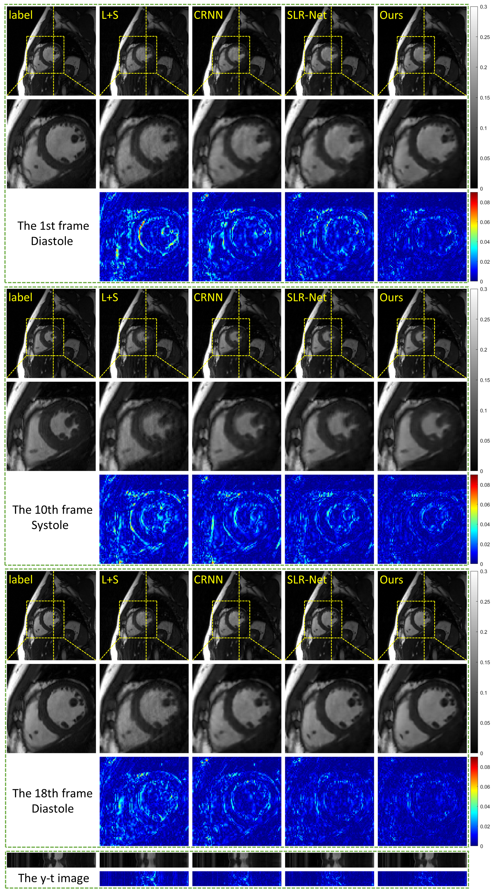
The reconstruction results of the single-channel data undersampled by 8-fold acceleration are shown in Fig. 2. From top to bottom (except the y-t image), Fig. 2 shows the reconstruction results of the 1st frame, the 10th frame, and the 18th frame to represent the dynamic images both in diastole and systole. The first row of each frame shows the reconstruction results of L+S, CRNN, SLR-Net, and PS-Net. The second row shows the zoomed-in view of the ROI region (indicated by the yellow box in the first row), and the third row shows the error map of the ROI region. The y-t image in the bottom shows the 92nd slice along the and temporal direction. The error range of the error map is [0–0.09].

The enlarged ROI region in the second row of the 1st and the 18th frame (the diastolic phase) suggest that PS-Net clearly reconstructs the tiny structures of papillary muscle without artifacts and outperforms other methods in detail retention and artifact removal. The error map of the reconstruction in the fifth row along the temporal dimension shows that PS-Net also outperforms the other methods in the dynamic map reconstruction. The reconstructed images of the 10th frame (the systolic phase) are not as good as the 1st and the 18th frame. Although all images are blurred due to high undersampling rate in the 10th frame, the PS-Net achieves the lowest errors with no significant deformation appears in the reconstructed results.
Compared with SLR-Net, which learns low-rank by the singular value soft threshold (SVT), we found that PS-Net is more accurate for low-rank learning, indicating that our adaptive low-rank learning strategy outperforms the representing low-rank prior by the hand-crafted nuclear norm.
We also performed the experiments at higher acceleration rates with 10-fold and 12-fold. The results are shown in Fig. 3. PS-Net clearly reconstructs the tiny structures of papillary muscle even at 12-fold acceleration. The quantitative evaluation metrics are shown in Table I, and it can be seen that the performance of PS-Net outperforms the state-of-the-art methods.
| AF | Methods | MSE(*e-5) | PSNR (dB) | SSIM(*e-2) |
|---|---|---|---|---|
| 8 | L+S | 11.54 5.12 | 39.75 1.75 | 94.46 1.68 |
| CRNN | 5.60 1.67 | 42.70 1.24 | 97.07 0.61 | |
| SLR-Net | 4.82 1.90 | 43.48 1.62 | 97.40 0.73 | |
| PS-Net | 2.91 1.25 | 45.74 1.78 | 98.19 0.64 | |
| 10 | L+S | 113.26 25.71 | 29.57 0.97 | 86.47 1.41 |
| CRNN | 7.28 2.25 | 41.58 1.31 | 96.49 0.75 | |
| SLR-Net | 8.07 2.86 | 41.19 1.49 | 95.94 0.94 | |
| PS-Net | 4.29 1.70 | 43.99 1.65 | 97.63 0.77 | |
| 12 | L+S | 113.42 25.90 | 29.56 0.90 | 86.46 1.45 |
| CRNN | 11.87 3.35 | 39.43 1.21 | 94.57 0.89 | |
| SLR-Net | 9.42 3.60 | 40.53 1.50 | 95.35 1.05 | |
| PS-Net | 5.29 2.09 | 43.09 1.67 | 97.16 0.89 |
III-B2 Multi-channel reconstruction results

In the multi-channel scenario, comparisons were made with the L+S method[36], and the model-driven based methods MoDL[15] and SLR-Net[14]. Because multi-channel data contains redundant information such as coil sensitivity, multi-channel data can be accelerated to a higher rate. The reconstruction results of multi-channel data undersampling with 12-fold acceleration are shown in Fig. 4, and the quantitative evaluation metrics are shown in Table II. In the multi-channel case, the reconstruction result of PS-Net outperforms the L+S, MoDL, and SLR-Net in terms of detail description, artifact removal, etc.
| AF | Methods | MSE(*e-5) | PSNR (dB) | SSIM(*e-2) |
|---|---|---|---|---|
| 12 | L+S | 20.89 13.54 | 37.52 2.35 | 93.31 3.47 |
| MoDL | 6.14 2.64 | 42.46 1.67 | 96.29 0.98 | |
| SLR-Net | 6.75 3.31 | 42.15 1.90 | 96.58 1.08 | |
| PS-Net | 3.67 1.89 | 44.87 2.07 | 98.04 0.85 |
III-B3 Ablation experiments

| AF | Methods | MSE(*e-5) | PSNR (dB) | SSIM(*e-2) |
|---|---|---|---|---|
| 12 | PS-Net(SVT) | 5.92 3.13 | 42.81 2.12 | 97.29 1.07 |
| Sparse-Net | 5.64 2.86 | 42.98 2.03 | 97.37 0.98 | |
| LowRank-Net | 4.97 2.36 | 43.47 1.92 | 97.12 1.02 | |
| PS-Net | 3.67 1.89 | 44.87 2.07 | 98.04 0.85 |
We designed ablation experiments to verify that adaptive low-rank learning strategy in PS-Net is effective. Three network were performed. The first one uses the SVT strategy to depict the low rank, implemented as the SVT module, which replaces the PS annihilation module, and the sparse module remains unchanged. This network is referred to as PS-Net (SVT). The second one removes the PS annihilation module, and the other modules and initialized hyper-parameters were kept unchanged, called Sparse-Net. The third one removes the sparse module and still uses the PS annihilation module for low-rank adaptive learning, named LowRank-Net. The initialization hyper-parameters of the above three networks are the same as PS-Net. The ablation experiments were performed in the multi-channel scenario with 12-fold acceleration. The reconstruction results are shown in Fig. 5. PS-Net reconstructs the papillary muscle more clearly and more detailed than PS-Net (SVT), without artifacts. And the error map of PS-Net in third row and fifth row are clearer than PS-Net (SVT), which indicates that our adaptive low-rank learning strategy effectively portrays the low-rank of dynamic MR images more accurately. The reconstruction effect of LowRank-Net is better than that of PS-Net(SVT), Sparse-Net, which also shows that our adaptive low-rank learning strategy is effective. After adding the sparse prior, the reconstruction result of PS-Net achieves the best result among the four networks. Table III shows the quantitative metrics of the reconstruction.
IV Discussion
IV-A Robustness experiments

| Methods | AF | MSE(*e-5) | PSNR (dB) | SSIM(*e-2) |
|---|---|---|---|---|
| PS-Net | 16 | 6.72 3.27 | 42.21 2.04 | 97.08 1.12 |
| 20 | 7.89 4.06 | 41.54 2.09 | 96.75 1.27 | |
| 24 | 9.36 4.58 | 40.78 2.01 | 96.25 1.40 |
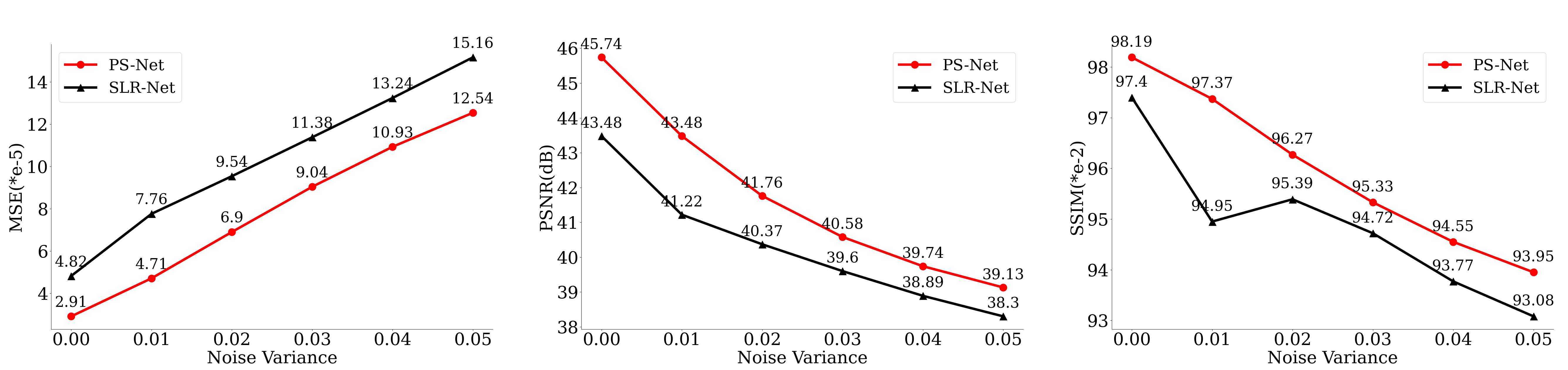
PS-Net represents the image by subspace, which can be seen as the generalization of PCA[38]. Hence PS-Net is more robust. The robustness of PS-Net is tested by artificially adding Gaussian white noise to the data during training and testing data. Fig. 6 shows the reconstruction results after adding Gaussian white noise with a variance of 0.01[39]. The enlarged view of the second row in Fig. 6 indicates that PS-Net sketches the papillary muscle boundary clearly and generates no artifacts in the core regions of the left and right ventricles, which are closer to the fully sampled label than SLR-Net. Besides, we conducted experiments with variance ranging from 0 to 0.05, and the quantitative metrics are shown in Fig. 7. The quantitative metrics show that PS-Net suppress noise well even in the harsh case of noise variance of 0.05.
IV-B Higher Acceleration Reconstruction
We also tested the performance of PS-Net at higher accelerations (16-fold, 20-fold, and 24-fold) with multi-coli data. The reconstruction results are shown in Fig. 8, and the quantitative metrics are illustrated in Table IV. The enlarged view of the ROI region in the second row of Fig. 8 indicates that PS-Net can reconstruct the papillary muscle outlines even at 24-fold, and no artifacts are generated in either the left or right ventricular regions.

IV-C Limitation
Since our method exploits the equivalence of Hankel matrix multiplication and convolution, there are more convolutional layers in PS-Net than other model-driven reconstruction-based methods, resulting in the network needing to be trained with 10 million parameters. Besides, although PS-Net shortens the reconstruction time of dynamic MRI, its reconstruction time remains close to SLR-Net. It does not reflect the time advantage of avoiding SVD calculation. The reason is that PS-Net has more convolutional layers, which causes the computation to take more time, offsetting the time advantage of avoiding SVD computation.
V Conclusion
This paper proposed a partially separable network (PS-Net) to more adaptively characterize the low-rank prior through a learnable null space transform. The null space transform was formulated as a Hankel matrix multiplication, equivalent to the convolution operation, and can be naturally unrolled into a convolutional network module. The ablation experiments show that the learnable low-rank representation enhances the low-rank characterization of the image than the nuclear norm and the reconstruction result is further improved by adding the sparse modules. Moreover, PS-Net has strong robustness and can suppress artifacts well. The experiments show that our method achieves the best reconstruction quality and quantitative evaluation metrics among the traditional compressed sensing method L+S, the deep learning end-to-end method CRNN, the model-driven based method MoDL and SLR-Net.
Acknowledgement
This study was supported in part by the National Key R&D Program of China nos. 2020YFA0712200, 2017YFC0108802, National Natural Science Foundation of China under grant nos. 62125111, 81830056, U1805261, 61671441, 81971611, 81901736, and the Innovation and Technology Commission of the government of Hong Kong SAR under grant no. MRP/001/18X, the Key Laboratory for Magnetic Resonance and Multimodality Imaging of Guangdong Province under grant no. 2020B1212060051, the Guangdong Basic and Applied Basic Research Foundation no. 2021A1515110540, and by the Chinese Academy of Sciences program under grant no. 2020GZL006.
References
- [1] D. Liang, J. Cheng, Z. Ke, and L. Ying, “Deep magnetic resonance image reconstruction: Inverse problems meet neural networks,” IEEE Signal Processing Magazine, vol. 37, no. 1, pp. 141–151, 2020.
- [2] G. Wang, J. C. Ye, K. Mueller, and J. A. Fessler, “Image reconstruction is a new frontier of machine learning,” IEEE Transactions on Medical Imaging, vol. 37, no. 6, pp. 1289–1296, 2018.
- [3] B. Zhu, J. Z. Liu, S. F. Cauley, B. R. Rosen, and M. S. Rosen, “Image reconstruction by domain-transform manifold learning,” Nature, vol. 555, no. 7697, pp. 487–492, 2018.
- [4] S. Wang, Z. Su, L. Ying, X. Peng, S. Zhu, F. Liang, D. Feng, and D. Liang, “Accelerating magnetic resonance imaging via deep learning,” in 2016 IEEE 13th International Symposium on Biomedical Imaging. IEEE, 2016, pp. 514–517.
- [5] K. Kwon, D. Kim, and H. Park, “A parallel mr imaging method using multilayer perceptron,” Medical Physics, vol. 44, no. 12, pp. 6209–6224, 2017.
- [6] Y. Han, J. Yoo, H. H. Kim, H. J. Shin, K. Sung, and J. C. Ye, “Deep learning with domain adaptation for accelerated projection-reconstruction mr,” Magnetic Resonance in Medicine, vol. 80, no. 3, pp. 1189–1205, 2018.
- [7] J. Schlemper, J. Caballero, J. V. Hajnal, A. N. Price, and D. Rueckert, “A deep cascade of convolutional neural networks for dynamic mr image reconstruction,” IEEE Transactions on Medical Imaging, vol. 37, no. 2, pp. 491–503, 2017.
- [8] Y. Yang, J. Sun, H. Li, and Z. Xu, “Admm-csnet: A deep learning approach for image compressive sensing,” IEEE Transactions on Pattern Analysis and Machine Intelligence, vol. 42, no. 3, pp. 521–538, 2018.
- [9] C. Qin, J. Schlemper, J. Caballero, A. N. Price, J. V. Hajnal, and D. Rueckert, “Convolutional recurrent neural networks for dynamic mr image reconstruction,” IEEE Transactions on Medical Imaging, vol. 38, no. 1, pp. 280–290, 2018.
- [10] C. M. Sandino, P. Lai, S. S. Vasanawala, and J. Y. Cheng, “Accelerating cardiac cine mri using a deep learning-based espirit reconstruction,” Magnetic Resonance in Medicine, vol. 85, no. 1, pp. 152–167, 2021.
- [11] Y. Liu, Q. Liu, M. Zhang, Q. Yang, S. Wang, and D. Liang, “Ifr-net: Iterative feature refinement network for compressed sensing mri,” IEEE Transactions on Computational Imaging, vol. 6, pp. 434–446, 2019.
- [12] T. Eo, Y. Jun, T. Kim, J. Jang, H.-J. Lee, and D. Hwang, “Kiki-net: cross-domain convolutional neural networks for reconstructing undersampled magnetic resonance images,” Magnetic Resonance in Medicine, vol. 80, no. 5, pp. 2188–2201, 2018.
- [13] J. Cheng, H. Wang, L. Ying, and D. Liang, “Model learning: Primal dual networks for fast mr imaging,” in International Conference on Medical Image Computing and Computer-Assisted Intervention. Springer, 2019, pp. 21–29.
- [14] Z. Ke, W. Huang, Z.-X. Cui, J. Cheng, S. Jia, H. Wang, X. Liu, H. Zheng, L. Ying, Y. Zhu et al., “Learned low-rank priors in dynamic mr imaging,” IEEE Transactions on Medical Imaging, vol. 40, no. 12, pp. 3698–3710, 2021.
- [15] H. K. Aggarwal, M. P. Mani, and M. Jacob, “Modl: Model-based deep learning architecture for inverse problems,” IEEE Transactions on Medical Imaging, vol. 38, no. 2, pp. 394–405, 2018.
- [16] W. Huang, Z. Ke, Z.-X. Cui, J. Cheng, Z. Qiu, S. Jia, L. Ying, Y. Zhu, and D. Liang, “Deep low-rank plus sparse network for dynamic mr imaging,” Medical Image Analysis, vol. 73, p. 102190, 2021.
- [17] J. Cheng, Z.-X. Cui, W. Huang, Z. Ke, L. Ying, H. Wang, Y. Zhu, and D. Liang, “Learning data consistency and its application to dynamic mr imaging,” IEEE Transactions on Medical Imaging, vol. 40, no. 11, pp. 3140–3153, 2021.
- [18] Z. Ke, Z.-X. Cui, W. Huang, J. Cheng, S. Jia, L. Ying, Y. Zhu, and D. Liang, “Deep manifold learning for dynamic mr imaging,” IEEE Transactions on Computational Imaging, vol. 7, pp. 1314–1327, 2021.
- [19] S. Ravishankar, B. E. Moore, R. R. Nadakuditi, and J. A. Fessler, “Low-rank and adaptive sparse signal (lassi) models for highly accelerated dynamic imaging,” IEEE Transactions on Medical Imaging, vol. 36, no. 5, pp. 1116–1128, 2017.
- [20] Z. Chen, Y. Fu, Y. Xiang, J. Xu, and R. Rong, “A novel low-rank model for mri using the redundant wavelet tight frame,” Neurocomputing, vol. 289, pp. 180–187, 2018.
- [21] C. Liao, Y. Chen, X. Cao, S. Chen, H. He, M. Mani, M. Jacob, V. Magnotta, and J. Zhong, “Efficient parallel reconstruction for high resolution multishot spiral diffusion data with low rank constraint,” Magnetic Resonance in Medicine, vol. 77, no. 3, pp. 1359–1366, 2017.
- [22] X. Zhang, Q. Lian, Y. Yang, and Y. Su, “A deep unrolling network inspired by total variation for compressed sensing mri,” Digital Signal Processing, vol. 107, p. 102856, 2020.
- [23] A. Bustin, N. Fuin, R. M. Botnar, and C. Prieto, “From compressed-sensing to artificial intelligence-based cardiac mri reconstruction,” Frontiers in Cardiovascular Medicine, vol. 7, p. 17, 2020.
- [24] Z.-p. Liang, “Spatiotemporal imagingwith partially separable functions,” in 2007 4th IEEE International Symposium on Biomedical Imaging, 2007, pp. 988–991.
- [25] M. Vetterli, P. Marziliano, and T. Blu, “Sampling signals with finite rate of innovation,” IEEE Transactions on Signal Processing, vol. 50, no. 6, pp. 1417–1428, 2002.
- [26] S. G. Lingala, Y. Hu, E. DiBella, and M. Jacob, “Accelerated dynamic mri exploiting sparsity and low-rank structure: k-t slr,” IEEE Transactions on Medical Imaging, vol. 30, no. 5, pp. 1042–1054, 2011.
- [27] C. Y. Lin and J. A. Fessler, “Efficient dynamic parallel mri reconstruction for the low-rank plus sparse model,” IEEE Transactions on Computational Imaging, vol. 5, no. 1, pp. 17–26, 2019.
- [28] A. Majumdar, “Improving synthesis and analysis prior blind compressed sensing with low-rank constraints for dynamic mri reconstruction,” Magnetic Resonance Imaging, vol. 33, no. 1, pp. 174–179, 2015.
- [29] A. Pramanik, H. K. Aggarwal, and M. Jacob, “Deep generalization of structured low-rank algorithms (deep-slr),” IEEE Transactions on Medical Imaging, vol. 39, no. 12, pp. 4186–4197, 2020.
- [30] X. Glorot, A. Bordes, and Y. Bengio, “Deep sparse rectifier neural networks,” in Proceedings of the Fourteenth International Conference on Artificial Intelligence and Statistics, 2011, pp. 315–323.
- [31] D. P. Kingma and J. Ba, “Adam: A method for stochastic optimization,” arXiv preprint arXiv:1412.6980, 2014.
- [32] M. Abadi, P. Barham, J. Chen, Z. Chen, A. Davis, J. Dean, M. Devin, S. Ghemawat, G. Irving, M. Isard et al., “Tensorflow: A system for large-scale machine learning,” in 12th USENIX symposium on Operating Systems Design and Implementation (OSDI 16), 2016, pp. 265–283.
- [33] H. Jung, J. C. Ye, and E. Y. Kim, “Improved k–t blast and k–t sense using focuss,” Physics in Medicine & Biology, vol. 52, no. 11, p. 3201, 2007.
- [34] R. Ahmad, H. Xue, S. Giri, Y. Ding, J. Craft, and O. P. Simonetti, “Variable density incoherent spatiotemporal acquisition (vista) for highly accelerated cardiac mri,” Magnetic Mesonance in Medicine, vol. 74, no. 5, pp. 1266–1278, 2015.
- [35] Z. Wang, A. C. Bovik, H. R. Sheikh, and E. P. Simoncelli, “Image quality assessment: from error visibility to structural similarity,” IEEE Transactions on Image Processing, vol. 13, no. 4, pp. 600–612, 2004.
- [36] R. Otazo, E. Candes, and D. K. Sodickson, “Low-rank plus sparse matrix decomposition for accelerated dynamic mri with separation of background and dynamic components,” Magnetic Resonance in Medicine, vol. 73, no. 3, pp. 1125–1136, 2015.
- [37] C. Qin, J. Schlemper, J. Caballero, A. N. Price, J. V. Hajnal, and D. Rueckert, “Convolutional recurrent neural networks for dynamic mr image reconstruction,” IEEE Transactions on Medical Imaging, vol. 38, no. 1, pp. 280–290, 2018.
- [38] N. Vaswani, T. Bouwmans, S. Javed, and P. Narayanamurthy, “Robust subspace learning: Robust pca, robust subspace tracking, and robust subspace recovery,” IEEE signal processing magazine, vol. 35, no. 4, pp. 32–55, 2018.
- [39] P. Zhuang, X. Zhu, and X. Ding, “Mri reconstruction with an edge-preserving filtering prior,” Signal Processing, vol. 155, pp. 346–357, 2019.