This paper was converted on www.awesomepapers.org from LaTeX by an anonymous user.
Want to know more? Visit the Converter page.

Proving some conjectures on Kekulé numbers for certain benzenoids by using Chebyshev polynomials

Guoce Xin1,∗ and Yueming Zhong2 1,2School of Mathematical Sciences, Capital Normal University, Beijing 100048, PR China 1guoce_xin@163.com & 2zhongyueming107@gmail.com
Abstract.

In chemistry, Cyvin-Gutman enumerates Kekulé numbers for certain benzenoids and record it as A050446A050446 on OEIS. This number is exactly the two variable array T(n,m)T(n,m) defined by the recursion T(n,m)=T(n,m1)+k=0n12T(2k,m1)T(n12k,m)T(n,m)=T(n,m-1)+\sum^{\lfloor\frac{n-1}{2}\rfloor}_{k=0}T(2k,m-1)T(n-1-2k,m), where T(n,0)=T(0,m)=1T(n,0)=T(0,m)=1 for all nonnegative integers m,nm,n. Interestingly, this number also appeared in the context of weighted graphs, graph polytopes, magic labellings, and unit primitive matrices, studied by different authors. Several interesting conjectures were made on the OEIS. These conjectures are related to both the row and column generating function of T(n,m)T(n,m). In this paper, give explicit formula of the column generating function, which is also the generating function F(n,x)F(n,x) studied by Bóna, Ju, and Yoshida. We also get trig function representations by using Chebyshev polynomials of the second kind. This allows us to prove all these conjectures.

* This work was partially supported by NSFC(12071311).

Mathematic subject classification: Primary 05A15; Secondary 15A18, 05C78, 52B11.

Keywords: Chebyshev polynomials; Kekulé numbers; unit-primitive matrix; linear graphs.

1. Introduction

Throughout this paper, we use standard set notations ,\mathbb{N},\mathbb{P} for nonnegative integers, and positive integers, respectively. We also use χ(true)=1\chi(true)=1 and χ(false)=0\chi(false)=0.

Definition 1.1.

The two parameter sequence A050446A050446 on [9] is defined by

(1.1) T(n,m)=T(n,m1)+k=0n12T(2k,m1)T(n12k,m),mT(n,m)=T(n,m-1)+\sum^{\lfloor\frac{n-1}{2}\rfloor}_{k=0}T(2k,m-1)T(n-1-2k,m),\qquad m\in\mathbb{P}

with initial condition T(n,0)=1T(n,0)=1 for all nn\in\mathbb{N}.

Table 1 gives the first several values of T(n,m)T(n,m) as the (n,m)(n,m) entries.

nn mm 0 1 2 3 4 5 6 7 8 9
0 1 1 1 1 1 1 1 1 1 1
1 1 2 3 4 5 6 7 8 9 10
2 1 3 6 10 15 21 28 36 45 55
3 1 5 14 30 55 91 140 204 285 385
4 1 8 31 85 190 371 658 1086 1695 2530
5 1 13 70 246 671 1547 3164 5916 10317 17017
Table 1. The first values of T(n,m)=K{z(n,m)}.T(n,m)=K\{z(n,m)\}.

One can find many interesting properties about T(n,m)T(n,m) on [9]. It counts certain chemistry structure, and several combinatorial structures as we shall introduce. Let

T(x,m)=n0T(n,m)xn,T(n,y)=m0T(n,m)ymT(x,m)=\sum_{n\geq 0}T(n,m)x^{n},\qquad T(n,y)=\sum_{m\geq 0}T(n,m)y^{m}

be the row and column generating function of T(n,m)T(n,m), respectively. There are six conjectures related to T(x,m)T(x,m) and T(n,y)T(n,y). We will state them in Section 2 after introducing some notations.

1.1. Kekulé structures
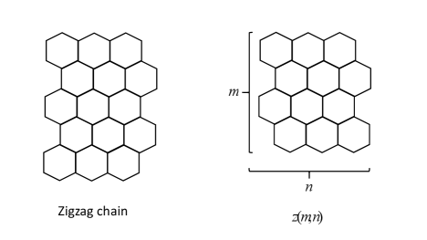
The number T(n,m)T(n,m) appeared in chemistry [3] as the number K{z(n,m)}K\{z(n,m)\} of Kekulé structures of the benzenoid hydrocarbon z(n,m)z(n,m), where z(n,m)z(n,m) is a zigzag chain interpreted as nn tier condensed linear chains (rows) of mm hexagons each in a zigzag arrangement as in Figure 1.
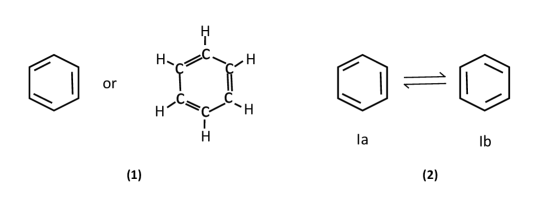
Refer to caption
Figure 1. Zigzag chain and z(m,n)z(m,n)

The special case z(1,1)z(1,1) is the single structure of benzene (C6H6C_{6}H_{6}). In Figure 2, picture (1) illustrates C6H6C_{6}H_{6}, and picture (2) gives the two Kekulé structures regarded differently in chemistry.
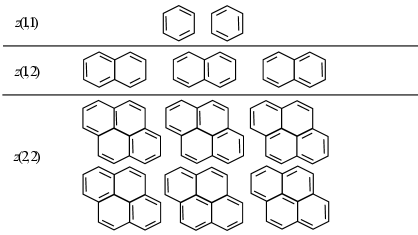
Refer to caption
Figure 2. Structural formula of benzene and its two Kekulé structures

The explicit definition of K{z(n,m)}K\{z(n,m)\} is too involved so we only give several of them in Figure 3. We cannot find a reference proving that K{z(n,m)}=T(n,m)K\{z(n,m)\}=T(n,m).

Refer to caption
Figure 3. The representation of the Kekulé structures of K{z(1,1)}K\{z(1,1)\}, K{z(1,2)}K\{z(1,2)\} and K{z(2,2)}K\{z(2,2)\}.

1.2. Combinatorial Models

Let G=(V,E)G=(V,E) be a simple graph with vertex set V={v1,v2,,vn}V=\{v_{1},v_{2},...,v_{n}\} and edge set EE. We will introduce three combinatorial models: i) Graph polytope studied in [8, 11, 15]; ii) Weighted graph studied in [1]; iii) Magic labellings of a graph studied in [13]. Though the concepts are for general graphs, we will focus on the linear graph (or path) LnL_{n} with nn vertices.

The graph polytope P(G)P(G) associated to a simple graph GG is defined as

P(G)={(x1,,xn)[0,1]nvivjExi+xj1}.P(G)=\{(x_{1},\dots,x_{n})\in[0,1]^{n}\mid v_{i}v_{j}\in E\Rightarrow x_{i}+x_{j}\leq 1\}.

The dilation of P(G)P(G) by mm is denoted mP(G)mP(G). The Ehrhart series of P(G)P(G) is defined by

Ehr(G)=Ehr(G,x)=1+m1|(mP(G)n)|xm.Ehr(G)=Ehr(G,x)=1+\sum_{m\geq 1}|(mP(G)\cap\mathbb{N}^{n})|x^{m}.

See [8, 11] for further references.

A a weighted graph of GG with distribution α=(m1,m2,,mn)n\alpha=(m_{1},m_{2},...,m_{n})\in\mathbb{N}^{n} is a triplet WGα=(V,E,α)WG_{\alpha}=(V,E,\alpha), where the weight of viv_{i} is mim_{i}. It is natural to define the weight of an edge vivjEv_{i}v_{j}\in E to be mi+mjm_{i}+m_{j}. Let WG(m)WG(m) be the number of all weighted graphs of GG with a fixed upper bound mm for weight of each vertex and edge of GG. That is, mi[m]:={0,1,2,,m}m_{i}\in[m]:=\{0,1,2,...,m\} for all ii and

(1.2) mi+mjm if vivjE.m_{i}+m_{j}\leq m\text{\ if\ }v_{i}v_{j}\in E.

An interesting question is to compute the generating function of WG(m)WG(m):

ρ(G)=ρ(G,x)=m=0WG(m)xm.\rho(G)=\rho(G,x)=\sum\limits_{m=0}^{\infty}WG(m)x^{m}.

Let G=(V,E)G=(V,E) be a finite (undirected) graph with vertex set V={v1,,vn}V=\{v_{1},\dots,v_{n}\} and edge set EE. We allow loops in EE so GG is also called a pseudo graph in the terminology of [6]. A magic labelling of GG with magic sum ss is a labelling of the edges in EE by nonnegative integers such that for each vertex vVv\in V, the weight wt(v)wt(v) of vv, defined to be the sum of labels of all edges incident to vv, is equal to ss. Denote by MG(s)M_{G}(s) the number of magic labelling of GG with magic sum ss. More precisely, MG(s)M_{G}(s) counts the number of maps μ:E\mu:E\mapsto\mathbb{N} satisfying

(1.3) wt(vi):=vivjEμ(vi,vj)=s,i=1,2,,n.\displaystyle wt(v_{i}):=\sum_{v_{i}v_{j}\in E}\mu(v_{i},v_{j})=s,\qquad i=1,2,\dots,n.

An interesting question is compute the generating function

(G)=(G,x)=s0MG(s)xs.\mathcal{M}(G)=\mathcal{M}(G,x)=\sum_{s\geq 0}M_{G}(s)x^{s}.

Finally, let Am=(ai,j)A_{m}=(a_{i,j}) be the order mm matrix defined by ai,j=χ(i+jm+1)a_{i,j}=\chi(i+j\leq m+1). It is called a unit-primitive matrix by Jeffery [7] in a different context.

The following result is claimed on [9], but we cannot find a real proof in the literature.

Theorem 1.2.

For (n,m)2(n,m)\in\mathbb{N}^{2}, the number T(n,m)T(n,m) has the following interpretations.

  1. (1)

    The (1,1)(1,1) entry of the matrix Am+1n+1A_{m+1}^{n+1}, also equal to um+1TAm+1n1um+1u_{m+1}^{T}A_{m+1}^{n-1}u_{m+1}, where um=(1,1,,1)Tmu_{m}=(1,1,\dots,1)^{T}\in\mathbb{N}^{m}.

  2. (2)

    The number WLn(m)WL_{n}(m) of weighted graphs of LnL_{n} with a fixed upper bound mm.

  3. (3)

    The number of integer lattice points in the dilated graph polytope mP(Ln)mP(L_{n}).

  4. (4)

    The number of magic labellings of the pseudo graph L~n\tilde{L}_{n} with magic sum mm, where L~n\tilde{L}_{n} is obtained from the linear graph Ln+1L_{n+1} by attaching one loop at each vertex.

Consequently in terms of generating functions, we have

T(n,x)=m0T(n,m)xm=Ehr(Ln)=ρ(Ln)=(L~n).\displaystyle T(n,x)=\sum_{m\geq 0}T(n,m)x^{m}=Ehr({L_{n}})=\rho(L_{n})=\mathcal{M}(\tilde{L}_{n}).

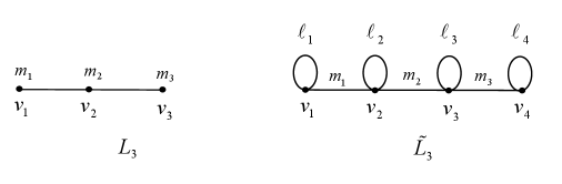
The equivalence of (2), (3), (4) can be easily seen by an example of m=3m=3. By definition, WL3(m)WL_{3}(m) is the number of \mathbb{N}-solutions α=(m1,m2,m3)\alpha=(m_{1},m_{2},m_{3}) of the system m1+m2m,m2+m3mm_{1}+m_{2}\leq m,\ m_{2}+m_{3}\leq m. The α\alpha’s are exactly the lattice points of the mm dilated graph polytope P(L3)={(x1,x2,x3):x1+x21,x2+x31}P(L_{3})=\{(x_{1},x_{2},x_{3})\in\mathbb{R}:x_{1}+x_{2}\leq 1,\ x_{2}+x_{3}\leq 1\}. Let 1=mm1,2=mm1m2,3=mm2m3,4=mm3\ell_{1}=m-m_{1},\ell_{2}=m-m_{1}-m_{2},\ell_{3}=m-m_{2}-m_{3},\ell_{4}=m-m_{3}. Then the system is translated to

m1+1=m,2+m1+m2=m,3+m2+m3=m,4+m3=m,m_{1}+\ell_{1}=m,\ \ell_{2}+m_{1}+m_{2}=m,\ \ell_{3}+m_{2}+m_{3}=m,\ \ell_{4}+m_{3}=m,

which says the labelling as in Figure 4 is a magic labeling of L~3\tilde{L}_{3}.

Refer to caption
Figure 4. Weighted graph of L3L_{3} and magic labelling of L~3\tilde{L}_{3}.

To see that (2) is equivalent to (1), we describe α\alpha as a walk on the finite state [m][m] of the αi\alpha_{i}’s: first choose α1[m]\alpha_{1}\in[m], then choose α2\alpha_{2} to be any number in [mα1][m-\alpha_{1}], since we have the restriction α1+α2m\alpha_{1}+\alpha_{2}\leq m, and then choose α3\alpha_{3} to be any number in [mα2][m-\alpha_{2}] by the restriction α2+α3m\alpha_{2}+\alpha_{3}\leq m. The transfer matrix from the state of αi\alpha_{i} to the state of αi+1\alpha_{i+1} is just Am+1A_{m+1}, the unit primitive matrix of order m+1m+1. It then follows that WL3(m)=um+1TAm+12um+1WL_{3}(m)=u_{m+1}^{T}A_{m+1}^{2}u_{m+1}.

The transfer matrix idea was used in [1], where weighted graphs were systematically enumerated and the following beautiful formula about LnL_{n} was cited.

Theorem 1.3.

(Bóna et al. [2]). For m=0,1,2,m=0,1,2,..., let

F(m,x)=k=0WLk(m)xk=1+k=0(um+1TAm+1kum+1)xk+1.F(m,x)=\sum\limits_{k=0}^{\infty}WL_{k}(m)x^{k}=1+\sum\limits_{k=0}^{\infty}(u_{m+1}^{T}A_{m+1}^{k}u_{m+1})x^{k+1}.

Then

F(m,x)\displaystyle F(m,x) =1x+F(m1,x)=1x+1x+F(m2,x)\displaystyle=\frac{1}{-x+F(m-1,-x)}=\frac{1}{-x+\frac{1}{x+F(m-2,x)}}
:=[x,x,F(m2,x)],\displaystyle:=[-x,x,F(m-2,x)],

where F(0,x)=1/(x+1)=[x,1]F(0,x)=1/(-x+1)=[-x,1] and F(1,x)=(1+x)/(1xx2)=[x,x,1]F(1,x)=(1+x)/(1-x-x^{2})=[-x,x,1]. That is, F(m,x)=[x,x,x,x,,(1)m1x,1]F(m,x)=[-x,x,-x,x,...,(-1)^{m-1}x,1].

However, the cited paper was never finished (private communication), so it is necessary to give a proof.

1.3. Main Results

Our objectives in this paper is 4-folded.

Firstly, we give a proof of Theorem 1.2. For convenience, we use vm,iv_{m,i} to denote the ii-th unit column vector in m\mathbb{R}^{m}. Let T¯(n,m)=umTAmnvm,1=umTAmn1um\overline{T}(n,m)=u_{m}^{T}A_{m}^{n}v_{m,1}=u_{m}^{T}A_{m}^{n-1}u_{m}. Then it is sufficient to prove the following.

Theorem 1.4.

For m,nm,n\in\mathbb{N}, we have

(1.4) T(n,m)=T¯(n,m+1).T(n,m)=\overline{T}(n,m+1).

Secondly, we give two proofs of Theorem 1.3. Further more, we obtain trig function representation.

Theorem 1.5.

For nn\in\mathbb{P}, we have

F(n,x)=(1)n+1sin(n+1)θsinnθsin(n+2)θsin(n+1)θ=(1)n+1cos(2n+12θ)cos(2n+32θ),F(n,x)=(-1)^{n+1}\frac{\sin(n+1)\theta-\sin n\theta}{\sin(n+2)\theta-\sin(n+1)\theta}=(-1)^{n+1}\frac{\cos(\frac{2n+1}{2}\theta)}{\cos(\frac{2n+3}{2}\theta)},

where cosθ=(1)nx2\cos\theta=\frac{(-1)^{n}x}{2}.

Thirdly, we obtain a factorization of the characteristic polynomial fAnf_{A_{n}} of AnA_{n} as follows, where throughout the paper, we use fA(x)=|xInA|f_{A}(x)=|xI_{n}-A| to denote the characteristic polynomial of an order nn matrix AA.

Theorem 1.6.

For a given positive integer nn, we have

fAn(x)=|xInAn|=j=1n[x(1)n+1(2cos(2j1)π2n+1)1].f_{A_{n}}(x)=|xI_{n}-A_{n}|=\prod\limits_{j=1}^{n}\left[x-(-1)^{n+1}\left(2\cos\frac{(2j-1)\pi}{2n+1}\right)^{-1}\right].

Finally, we prove the six conjectures related to T(n,m)T(n,m) in Section 2.

1.4. Summary

This paper is organized as follows: In Section 2 we state the six conjectures after introducing some notations. Chebyshev polynomial of the second kind plays an important role in our development. Section 3 proves Theorem 1.4, an equivalent form of Theorem 1.2. The idea is to use matrix computation to derive certain recursion of T¯n,m\overline{T}_{n,m}. The idea is used to give a proof of Theorems 1.3, but seems irrelevant to the other sections. Section 4 studies many properties of the unit primitive matrix AnA_{n}, especially its eigenvalues. As consequences, we give the proof of Theorems 1.5-1.6 and Conjecture 1. We also give explicit formula of the column generating function T(x,m)=F(m,x)T(x,m)=F(m,x). In Section 5, we first use the magic labelling model to sketch a proof of Conjectures 2-3, which are related to the row generating function T(n,x)T(n,x). Conjectures 4-6 are about the numerator of T(n,x)T(n,x). We prove them in later subsections by using the explicit formulas of the column generating function T(x,m)T(x,m).

2. Six Conjectures Related to T(n,m)T(n,m)

We will introduce 6 interesting conjectures related to the unit-primitive matrix AnA_{n} and the sequence T(m,n)T(m,n). Their proofs will be given in later sections.

Our development highly relies on Chebyshev polynomial of the second kind (CPS for short), which is defined recursively by

U0(x)=1,U1(x)=2x,Un(x)=2xUn1(x)Un2(x).\displaystyle U_{0}(x)=1,\quad U_{1}(x)=2x,\quad U_{n}(x)=2xU_{n-1}(x)-U_{n-2}(x).

We also need the well-known formula (see, e.g., [10]):

(2.1) Un(x)=sin[(n+1)cos1x]sin(cos1x)=k=0n2(1)k(nkk)(2x)n2k.U_{n}(x)=\frac{\sin[(n+1)\cos^{-1}x]}{\sin(\cos^{-1}x)}=\sum\limits_{k=0}^{\lfloor\frac{n}{2}\rfloor}(-1)^{k}\binom{n-k}{k}(2x)^{n-2k}.

Many results are related to the polynomials Pn(x),nP_{n}(x),n\in\mathbb{P} defined by

(2.2) Pn(x)=k=0nP(n,k)xk=k=0n(1)3k2(n+k2k)xk.\displaystyle P_{n}(x)=\sum_{k=0}^{n}P(n,k)x^{k}=\sum_{k=0}^{n}(-1)^{\lfloor\frac{3k}{2}\rfloor}\binom{\lfloor\frac{n+k}{2}\rfloor}{k}x^{k}.

The first conjecture is related to the unit-primitive matrix AnA_{n}.

Conjecture 1.

(A187660 [9]). (i) For positive integer nn\in\mathbb{P}. The characteristic polynomial fAn(x)f_{A_{n}}(x) of the n×nn\times n unit-primitive matrix AnA_{n} is:

(2.3) fAn(x)=det(xInAn)=xnPn(1/x).\displaystyle f_{A_{n}}(x)=\det(xI_{n}-A_{n})=x^{n}P_{n}(1/x).

(ii) The nn eigenvalues of AnA_{n} are given by wn,j=Un1(δn,j)w_{n,j}=U_{n-1}(\delta_{n,j}), where δn,j=2cos(2j12n+1π)\delta_{n,j}=2\cos(\frac{2j-1}{2n+1}\pi) for j=1,,nj=1,...,n.

The other 5 conjectures are all related to the sequence T(n,m)T(n,m) defined by (1.1).

Let EnE_{n} be the Euler number [12, Section 3.16] with exponential generating function

sec(x)=n0E2n(2n)!x2n,tan(x)=n0E2n+1(2n+1)!x2n+1.\sec(x)=\sum_{n\geq 0}\frac{E_{2n}}{(2n)!}x^{2n},\qquad\tan(x)=\sum_{n\geq 0}\frac{E_{2n+1}}{(2n+1)!}x^{2n+1}.

The following result was observed in [9].

Lemma 2.1.

For fixed nonnegative integer nn, T(n,m)T(n,m) is a polynomial in mm of degree nn with leading coefficient n=En/n!\ell_{n}=E_{n}/n!. Therefore the nn-th row generating function of T(n,m)T(n,m) is of the following form

T(n,x)=m0T(n,m)xm=Hn(x)/(1x)n+1,T(n,x)=\sum_{m\geq 0}T(n,m)x^{m}=H_{n}(x)/(1-x)^{n+1},

where Hn(x)H_{n}(x) is a polynomial of degree no more than nn. Here we start with row 0.

Proof.

The reason is so simple that we include it here. For the first part, let pn(m)=T(n,m)p_{n}(m)=T(n,m). We need to show that pn(x)[x]p_{n}(x)\in\mathbb{Q}[x] with degpn(x)=n\deg p_{n}(x)=n and the leading coefficient is En/n!E_{n}/n!. The assertion clearly holds for n=0n=0, since p0(m)=1p_{0}(m)=1. Assume the lemma holds for all k<nk<n. To show the assertion holds for pn(m)p_{n}(m), we rewrite (1.1) as

Δ(pn(m))=pn(m)pn(m1)=k=0n12p2k(m1)pn12k(m).\displaystyle\Delta(p_{n}(m))=p_{n}(m)-p_{n}(m-1)=\sum^{\lfloor\frac{n-1}{2}\rfloor}_{k=0}p_{2k}(m-1)p_{n-1-2k}(m).

That is, the divided difference of pn(m)p_{n}(m) is a sum of polynomials of degree n1n-1 with leading coefficient

L=k=0n122kn12k=k=0n12E2k(2k)!En12k(n12k)!L=\sum^{\lfloor\frac{n-1}{2}\rfloor}_{k=0}\ell_{2k}\ell_{n-1-2k}=\sum^{\lfloor\frac{n-1}{2}\rfloor}_{k=0}\frac{E_{2k}}{(2k)!}\frac{E_{n-1-2k}}{(n-1-2k)!}

by the induction hypothesis. Therefore pn(m)p_{n}(m) is a polynomial in mm of degree nn with leading coefficient n=L/n\ell_{n}=L/n. It is in fact EnE_{n} follows by equating coefficient of xn1x^{n-1} in the identity ddx(sec(x)+tan(x))=sec(x)(sec(x)+tan(x)).\frac{\mathrm{d}}{\mathrm{d}x}(\sec(x)+\tan(x))=\sec(x)(\sec(x)+\tan(x)).

The second part follows by classical theory on rational functions. See [12].  

Simple calculation shows that H0(x)=H1(x)=1H_{0}(x)=H_{1}(x)=1. The second conjecture gives more details on Hn(x)H_{n}(x).

Conjecture 2.

(A205497 [9]). For n2n\geq 2, the numerator of the nn-th row generating function of T(n,m)T(n,m) is a polynomial of degree n2n-2. That is

Hn(x)=Mn2,0+Mn3,1x+Mn4,2x2++M0,n2xn2,H_{n}(x)=M_{n-2,0}+M_{n-3,1}x+M_{n-4,2}x^{2}+\cdots+M_{0,n-2}x^{n-2},

where Mn2j,jM_{n-2-j,j} is as in Table 2 below for j=0,1,,n2j=0,1,\dots,n-2.

The array Mi,jM_{i,j} is given by the sequence A205497 in [9]. Christopher H. Gribble kindly calculated the first 100 antidiagonals of the array MM which starts as in Table 2.

nn kk 0 1 2 3 4 5
0 1 1 1 1 1 1
1 1 3 7 14 26 46
2 1 7 31 109 334 937
3 1 14 109 623 2951 12331
4 1 26 334 2951 20641 123216
5 1 46 937 12331 123216 1019051
Table 2. The Mn,kM_{n,k}

There are several conjectures about Mi,jM_{i,j}.

Conjecture 3.

(A205497 [9]). Mn,k=Mk,nM_{n,k}=M_{k,n}, for all nn and kk; that is, MM is symmetric about the central terms {1,3,31,623,}\{1,3,31,623,...\}.

Conjecture 4.

(A205497 [9]). Assuming Conjecture 2, we have these following results.

  • (1)

    The generating function for row (or column) nn of MM is of the form

    (2.4) Gn(x)(P1(x))n+1(P2(x))n(Pn(x))2Pn+1(x).\frac{G_{n}(x)}{\left(P_{1}(x))^{n+1}(P_{2}(x))^{n}...(P_{n}(x)\right)^{2}P_{n+1}(x)}.
  • (2)

    The numerator Gn(x)G_{n}(x) is a polynomial of degree n(n+4)(n+5)6\frac{n(n+4)(n+5)}{6}(A005586(n)A005586(n), see [9]).

  • (3)

    The denominator (P1(x))n+1(P2(x))n(Pn(x))2Pn+1(x)(P_{1}(x))^{n+1}(P_{2}(x))^{n}...(P_{n}(x))^{2}P_{n+1}(x) is a polynomial of degree n(n+1)(n+2)6\frac{n(n+1)(n+2)}{6}(A000292(n+1)A000292(n+1), see [9]).

Conjecture 5.

(A205497 [9]). The generation functions from column 0 to 4 of MM are the following 5 in order.

  • (0)

    1/(1x)1/(1-x);

  • (1)

    1(1x)2(1xx2)\frac{1}{(1-x)^{2}(1-x-x^{2})};

  • (2)

    1x2x3x4+x5(1x)3(1xx2)2(12xx2+x3)\frac{1-x^{2}-x^{3}-x^{4}+x^{5}}{(1-x)^{3}(1-x-x^{2})^{2}(1-2x-x^{2}+x^{3})};

  • (3)

    1+x6x215x3+21x4+35x513x651x7+3x8+21x9+5x10+x115x12x13x14(1x)4(1xx2)3(12xx2+x3)2(12x3x2+x3+x4)\frac{1+x-6x^{2}-15x^{3}+21x^{4}+35x^{5}-13x^{6}-51x^{7}+3x^{8}+21x^{9}+5x^{10}+x^{11}-5x^{12}-x^{13}-x^{14}}{(1-x)^{4}(1-x-x^{2})^{3}(1-2x-x^{2}+x^{3})^{2}(1-2x-3x^{2}+x^{3}+x^{4})};

  • (4)

    N4(x)(1x)5(1xx2)4(12xx2+x3)3(12x3x2+x3+x4)2(13x3x2+4x3+x4x5)\frac{N_{4}(x)}{(1-x)^{5}(1-x-x^{2})^{4}(1-2x-x^{2}+x^{3})^{3}(1-2x-3x^{2}+x^{3}+x^{4})^{2}(1-3x-3x^{2}+4x^{3}+x^{4}-x^{5})}.

Here

N4(x)\displaystyle N_{4}(x) =1+4x31x267x3+348x4+418x51893x61084x7+4326x8+4295x97680x109172x11+9104x12\displaystyle=1+4x-31x^{2}-67x^{3}+348x^{4}+418x^{5}-1893x^{6}-1084x^{7}+4326x^{8}+4295x^{9}-7680x^{10}-9172x^{11}+9104x^{12}
+11627x135483x1410773x15+1108x16+7255x17+315x183085x19228x20+669x21+102x22\displaystyle+11627x^{13}-5483x^{14}-10773x^{15}+1108x^{16}+7255x^{17}+315x^{18}-3085x^{19}-228x^{20}+669x^{21}+102x^{22}
23x2345x2416x25+11x26+2x27x28.\displaystyle-23x^{23}-45x^{24}-16x^{25}+11x^{26}+2x^{27}-x^{28}.
Conjecture 6.

(A205497 [9]). Assuming Conjecture 2, we have

limnMn+1,mMn,m=Um(cos(π2m+3)).\mathrm{lim}_{n\rightarrow\infty}\frac{M_{n+1,m}}{M_{n,m}}=U_{m}\left(\cos\left(\frac{\pi}{2m+3}\right)\right).

This limit is also equal to spectral radius of the m×mm\times m unit-primitive matrix AmA_{m}, where identical limits for the columns of the transpose MTM^{T} of MM.

3. Proofs of Theorems 1.3 and 1.4

In this section, we first prove Theorem 1.4 by using matrix computations. Then we use similar idea to give our first proof of Theorem 1.3. The ideas in this section are irrelevant to the other sections.

We use the following notations: Xm=(vm,1,vm,2,,vm,m)X_{m}=(v_{m,1},v_{m,2},...,v_{m,m}), A¯m=AmXm\bar{A}_{m}=A_{m}-X_{m} and Jm=umumTJ_{m}=u_{m}u_{m}^{T} (the all 11 matrix). The basic properties of these order mm matrices are given in the following lemma. They will be used in the next subsection.

Lemma 3.1.

For a given positive integer mm, the following equations all hold true.

  • (1)

    A¯mXm+XmAm=Jm\bar{A}_{m}X_{m}+X_{m}A_{m}=J_{m} and XmA¯m+AmXm=JmX_{m}\bar{A}_{m}+A_{m}X_{m}=J_{m};

  • (2)

    Amvm,1=umA_{m}v_{m,1}=u_{m};

  • (3)

    umTXm=umTu_{m}^{T}X_{m}=u_{m}^{T};

  • (4)

    Amvm,1umT=JmA_{m}v_{m,1}u_{m}^{T}=J_{m};

  • (5)

    A¯mXmvm,1=0\bar{A}_{m}X_{m}v_{m,1}=0;

  • (6)

    AmXmvm,1=vm,1A_{m}X_{m}v_{m,1}=v_{m,1};

  • (7)

    umTA¯mvm,1=u¯mTA¯mvm,1=um1TAm1vm1,1u_{m}^{T}\bar{A}_{m}v_{m,1}=\bar{u}_{m}^{T}\bar{A}_{m}v_{m,1}=u_{m-1}^{T}A_{m-1}v_{m-1,1}, where u¯m=umvm,m\bar{u}_{m}=u_{m}-v_{m,m}.

Proof.

The first six equalities are straightforward, so we only prove the seventh equality. By using block matrix operation, we have

umTA¯mvm,1\displaystyle u_{m}^{T}\bar{A}_{m}v_{m,1} =(um1T,1)(Am1000)(vm1,10)\displaystyle=(u_{m-1}^{T},1)\begin{pmatrix}A_{m-1}&0\\ 0&0\end{pmatrix}\binom{v_{m-1,1}}{0}
=(um1TAm1,0)(vm1,10)\displaystyle=(u_{m-1}^{T}A_{m-1},0)\binom{v_{m-1,1}}{0}
=(umTvm,mT)A¯mvm,m=u¯mTA¯mvm,1\displaystyle=(u_{m}^{T}-v_{m,m}^{T})\bar{A}_{m}v_{m,m}=\bar{u}_{m}^{T}\bar{A}_{m}v_{m,1}
=um1TAm1vm1,1.\displaystyle=u_{m-1}^{T}A_{m-1}v_{m-1,1}.


3.1. Proof of Theorem 1.4

To prove Theorem 1.4, it is sufficient to show that T¯(n,m+1)\overline{T}(n,m+1) satisfy the same recursion (1.1) as for T(n,m)T(n,m). This is Corollary 3.6 below.

We need some lemmas.

Lemma 3.2.

Given three positive integers mm, nn and kk with 1kn21\leq k\leq n-2, we have

(3.1) A¯mkAmnkA¯mk+2Amnk2=A¯mk+1vm,1umTAmnk2.\bar{A}_{m}^{k}A^{n-k}_{m}-\bar{A}^{k+2}_{m}A_{m}^{n-k-2}=\bar{A}_{m}^{k+1}v_{m,1}u_{m}^{T}A_{m}^{n-k-2}.
Proof.
A¯mkAmnkA¯mk+2Amnk2\displaystyle\bar{A}_{m}^{k}A^{n-k}_{m}-\bar{A}^{k+2}_{m}A_{m}^{n-k-2}
=A¯mk(A¯m+Xm)Amnk1A¯mk+2Amnk2\displaystyle=\bar{A}_{m}^{k}(\bar{A}_{m}+X_{m})A_{m}^{n-k-1}-\bar{A}^{k+2}_{m}A_{m}^{n-k-2}
=A¯mk+1(A¯m+Xm)Amnk2+A¯mkXmAmnk1A¯mk+2Amnk2\displaystyle=\bar{A}_{m}^{k+1}(\bar{A}_{m}+X_{m})A_{m}^{n-k-2}+\bar{A}_{m}^{k}X_{m}A_{m}^{n-k-1}-\bar{A}^{k+2}_{m}A_{m}^{n-k-2}
=A¯mk+2Amnk2+A¯mk(A¯mXm+XmAm)Amnk2A¯mk+2Amnk2\displaystyle=\bar{A}_{m}^{k+2}A_{m}^{n-k-2}+\bar{A}_{m}^{k}(\bar{A}_{m}X_{m}+X_{m}A_{m})A_{m}^{n-k-2}-\bar{A}^{k+2}_{m}A_{m}^{n-k-2}
(by Lemma 3.1(1)) =A¯mkJmAmnk2\displaystyle=\bar{A}_{m}^{k}J_{m}A_{m}^{n-k-2}
(by Lemma 3.1(4)) =A¯mkAmvm,1umTAmnk2\displaystyle=\bar{A}_{m}^{k}A_{m}v_{m,1}u_{m}^{T}A_{m}^{n-k-2}
=A¯mk(A¯m+Xm)vm,1umTAmnk2\displaystyle=\bar{A}_{m}^{k}(\bar{A}_{m}+X_{m})v_{m,1}u_{m}^{T}A_{m}^{n-k-2}
=A¯mk+1vm,1umTAmnk2+A¯mkXmvm,1umTAmnk2\displaystyle=\bar{A}_{m}^{k+1}v_{m,1}u_{m}^{T}A_{m}^{n-k-2}+\bar{A}_{m}^{k}X_{m}v_{m,1}u_{m}^{T}A_{m}^{n-k-2}
(by Lemma 3.1(5)) =A¯mk+1vm,1umTAmnk2.\displaystyle=\bar{A}_{m}^{k+1}v_{m,1}u_{m}^{T}A_{m}^{n-k-2}.


Lemma 3.3.

For given two positive integers mm and nn, we have

umTA¯m2n12+1Amn2n121vm,1=umTA¯mnvm,1.u_{m}^{T}\bar{A}_{m}^{2\lfloor\frac{n-1}{2}\rfloor+1}A_{m}^{n-2\lfloor\frac{n-1}{2}\rfloor-1}v_{m,1}=u_{m}^{T}\bar{A}_{m}^{n}v_{m,1}.
Proof.

We discuss by the parity of nn as follows.

If nn is odd, then 2n12+1=n2\lfloor\frac{n-1}{2}\rfloor+1=n. We have

umTA¯m2n12+1Amn2n121vm,1=umTA¯mnvm,1.u_{m}^{T}\bar{A}_{m}^{2\lfloor\frac{n-1}{2}\rfloor+1}A_{m}^{n-2\lfloor\frac{n-1}{2}\rfloor-1}v_{m,1}=u_{m}^{T}\bar{A}_{m}^{n}v_{m,1}.

If nn is even, then 2n12+1=n12\lfloor\frac{n-1}{2}\rfloor+1=n-1. We have

umTA¯m2n12+1Amn2n121vm,1\displaystyle u_{m}^{T}\bar{A}_{m}^{2\lfloor\frac{n-1}{2}\rfloor+1}A_{m}^{n-2\lfloor\frac{n-1}{2}\rfloor-1}v_{m,1} =umTA¯mn1Amvm,1\displaystyle=u_{m}^{T}\bar{A}_{m}^{n-1}A_{m}v_{m,1}
=umTA¯mn1(A¯m+Xm)vm,1\displaystyle=u_{m}^{T}\bar{A}_{m}^{n-1}(\bar{A}_{m}+X_{m})v_{m,1}
(by Lemma 3.1(5)) =umTA¯mnvm,1.\displaystyle=u_{m}^{T}\bar{A}_{m}^{n}v_{m,1}.

This completes the proof.  

Lemma 3.4.

For given two positive integers mm and nn, we have

A¯mAmn1A¯m2n12+1Amn2n121+vm,1umTAmn1=i=0n12A¯m2ivm,1umTAmn12i.\bar{A}_{m}A_{m}^{n-1}-\bar{A}_{m}^{2\lfloor\frac{n-1}{2}\rfloor+1}A_{m}^{n-2\lfloor\frac{n-1}{2}\rfloor-1}+v_{m,1}u_{m}^{T}A_{m}^{n-1}=\sum\limits_{i=0}^{\lfloor\frac{n-1}{2}\rfloor}\bar{A}_{m}^{2i}v_{m,1}u_{m}^{T}A_{m}^{n-1-2i}.
Proof.

By adding Equation (3.1) with respect to k=1,3,,2n121k=1,3,...,2\lfloor\frac{n-1}{2}\rfloor-1, we get

(3.2) A¯mAmn1A¯m2n12+1Amn2n121=i=1n12A¯m2ivm,1umTAmn12i.\bar{A}_{m}A_{m}^{n-1}-\bar{A}_{m}^{2\lfloor\frac{n-1}{2}\rfloor+1}A_{m}^{n-2\lfloor\frac{n-1}{2}\rfloor-1}=\sum\limits_{i=1}^{\lfloor\frac{n-1}{2}\rfloor}\bar{A}_{m}^{2i}v_{m,1}u_{m}^{T}A_{m}^{n-1-2i}.

This is just a equivalent form of the lemma.  

A direct consequence of Lemma 3.4 is the following.

Theorem 3.5.

Let mm and nn be two positive integers. Then for any vectors 𝛂=(α1,.αm){\boldsymbol{\alpha}}=(\alpha_{1},....\alpha_{m}) and 𝛃=(β1,,βm){\boldsymbol{\beta}}=(\beta_{1},...,\beta_{m}), we have

𝜶TA¯mAmn1𝜷𝜶TA¯m2n12+1Amn2n121𝜷+𝜶Tvm,1umTAmn1𝜷=i=0n12𝜶TA¯m2ivm,1umTAmn12i𝜷.{\boldsymbol{\alpha}}^{T}\bar{A}_{m}A_{m}^{n-1}{\boldsymbol{\beta}}-{\boldsymbol{\alpha}}^{T}\bar{A}_{m}^{2\lfloor\frac{n-1}{2}\rfloor+1}A_{m}^{n-2\lfloor\frac{n-1}{2}\rfloor-1}{\boldsymbol{\beta}}+{\boldsymbol{\alpha}}^{T}v_{m,1}u_{m}^{T}A_{m}^{n-1}{\boldsymbol{\beta}}=\sum\limits_{i=0}^{\lfloor\frac{n-1}{2}\rfloor}{\boldsymbol{\alpha}}^{T}\bar{A}_{m}^{2i}v_{m,1}u_{m}^{T}A_{m}^{n-1-2i}{\boldsymbol{\beta}}.

In particular, setting 𝜶=um{\boldsymbol{\alpha}}=u_{m} and 𝜷=vm,1{\boldsymbol{\beta}}=v_{m,1} gives the following corollary.

Corollary 3.6.

For positive integers mm and nn, we have

(3.3) T¯(n,m)=T¯(n,m1)+k=0n12T¯(2k,m1)T¯(n2k1,m).\overline{T}(n,m)=\overline{T}(n,m-1)+\sum\limits_{k=0}^{\lfloor\frac{n-1}{2}\rfloor}\overline{T}(2k,m-1)\overline{T}(n-2k-1,m).
Proof.

It is easy to check that Equation (3.3) holds for n=1n=1. Now for n2n\geq 2, we have

T¯(n,m)\displaystyle\overline{T}(n,m) =umTAmnvm,1\displaystyle=u_{m}^{T}A_{m}^{n}v_{m,1}
=umT(A¯m+Xm)Amn1vm,1\displaystyle=u_{m}^{T}(\bar{A}_{m}+X_{m})A_{m}^{n-1}v_{m,1}
=umTA¯mAmn1vm,1+umTXmAmn1vm,1\displaystyle=u_{m}^{T}\bar{A}_{m}A_{m}^{n-1}v_{m,1}+u_{m}^{T}X_{m}A_{m}^{n-1}v_{m,1}
=umTA¯mAmn1vm,1+umTAmn1vm,1\displaystyle=u_{m}^{T}\bar{A}_{m}A_{m}^{n-1}v_{m,1}+u_{m}^{T}A_{m}^{n-1}v_{m,1}
(by Theorem 3.5) =umTA¯m2n12+1Amn2n121vm,1+i=0n12umTA¯m2ivm,1umTAmn12ivm,1\displaystyle=u_{m}^{T}\bar{A}_{m}^{2\lfloor\frac{n-1}{2}\rfloor+1}A_{m}^{n-2\lfloor\frac{n-1}{2}\rfloor-1}v_{m,1}+\sum\limits_{i=0}^{\lfloor\frac{n-1}{2}\rfloor}u_{m}^{T}\bar{A}_{m}^{2i}v_{m,1}u_{m}^{T}A_{m}^{n-1-2i}v_{m,1}
(by Lemma 3.3) =T¯(n,m1)+k=0n12T¯(2k,m1)T¯(n12k,m).\displaystyle=\overline{T}(n,m-1)+\sum^{\lfloor\frac{n-1}{2}\rfloor}_{k=0}\overline{T}(2k,m-1)\overline{T}(n-1-2k,m).


3.2. Proof of Theorem 1.3

We will prove a more general result by using similar technique as in the previous subsection.

Lemma 3.7.

For given three positive integers mm, nn and kk, we have

AmnkXmA¯mk+Amnk1XmA¯mk+1=Amnkvm,1umTA¯mk.A_{m}^{n-k}X_{m}\bar{A}_{m}^{k}+A_{m}^{n-k-1}X_{m}\bar{A}_{m}^{k+1}=A_{m}^{n-k}v_{m,1}u_{m}^{T}\bar{A}_{m}^{k}.
Proof.

We have

AmnkXmA¯mk+Amnk1XmA¯mk+1\displaystyle A_{m}^{n-k}X_{m}\bar{A}_{m}^{k}+A_{m}^{n-k-1}X_{m}\bar{A}_{m}^{k+1} =Amnk1(AmXm+XmA¯m)A¯mk\displaystyle=A_{m}^{n-k-1}(A_{m}X_{m}+X_{m}\bar{A}_{m})\bar{A}_{m}^{k}
(by Lemma 3.1(1)) =Amnk1JmA¯mk\displaystyle=A_{m}^{n-k-1}J_{m}\bar{A}_{m}^{k}
=Amnk1umumTA¯mk\displaystyle=A_{m}^{n-k-1}u_{m}u_{m}^{T}\bar{A}_{m}^{k}
(by Lemma 3.1(2)) =Amnkvm,1umTA¯mk.\displaystyle=A_{m}^{n-k}v_{m,1}u_{m}^{T}\bar{A}_{m}^{k}.


Lemma 3.8.

For given two positive integers mm and nn, we have

AmnXm+(1)n1XmA¯mn=k=0n1(1)kAmnkvm,1umTA¯mk.A_{m}^{n}X_{m}+(-1)^{n-1}X_{m}\bar{A}_{m}^{n}=\sum\limits_{k=0}^{n-1}(-1)^{k}A_{m}^{n-k}v_{m,1}u_{m}^{T}\bar{A}_{m}^{k}.
Proof.

By Lemma 3.7, we have

(3.4) (1)k(AmnkXmA¯mk+Amnk1XmA¯mk+1)=(1)kAmnkvm,1umTA¯mk.(-1)^{k}(A_{m}^{n-k}X_{m}\bar{A}_{m}^{k}+A_{m}^{n-k-1}X_{m}\bar{A}_{m}^{k+1})=(-1)^{k}A_{m}^{n-k}v_{m,1}u_{m}^{T}\bar{A}_{m}^{k}.

Adding Equation (3.6) with respect to k=0,,n1k=0,...,n-1 gives

AmnXm+(1)n1XmA¯mn=k=0n1(1)kAmnkvm,1umTA¯mk.A_{m}^{n}X_{m}+(-1)^{n-1}X_{m}\bar{A}_{m}^{n}=\sum\limits_{k=0}^{n-1}(-1)^{k}A_{m}^{n-k}v_{m,1}u_{m}^{T}\bar{A}_{m}^{k}.

This completes the proof.  

Lemma 3.9.

For given two positive integers mm and nn, we have

(3.5) AmnXm(1)nXmA¯mn+(1)nvm,1umTA¯mnAmnvm,1vm,mT=k=0n(1)kAmnkvm,1u¯mTA¯mk.A_{m}^{n}X_{m}-(-1)^{n}X_{m}\bar{A}_{m}^{n}+(-1)^{n}v_{m,1}u_{m}^{T}\bar{A}_{m}^{n}-A_{m}^{n}v_{m,1}v_{m,m}^{T}=\sum\limits_{k=0}^{n}(-1)^{k}A_{m}^{n-k}v_{m,1}\bar{u}_{m}^{T}\bar{A}_{m}^{k}.
Proof.

By Lemma 3.7, we have

(3.6) (1)k(AmnkXmA¯mk+Amnk1XmA¯mk+1)=(1)kAmnkvm,1umTA¯mk.(-1)^{k}(A_{m}^{n-k}X_{m}\bar{A}_{m}^{k}+A_{m}^{n-k-1}X_{m}\bar{A}_{m}^{k+1})=(-1)^{k}A_{m}^{n-k}v_{m,1}u_{m}^{T}\bar{A}_{m}^{k}.

Adding Equation (3.6) with respect to k=0,,n1k=0,...,n-1 gives

AmnXm+(1)n1XmA¯mn\displaystyle A_{m}^{n}X_{m}+(-1)^{n-1}X_{m}\bar{A}_{m}^{n} =k=0n1(1)kAmnkvm,1umTA¯mk\displaystyle=\sum\limits_{k=0}^{n-1}(-1)^{k}A_{m}^{n-k}v_{m,1}u_{m}^{T}\bar{A}_{m}^{k}
(by umTA¯m=u¯mTA¯m)\displaystyle(\text{by }u_{m}^{T}\bar{A}_{m}=\bar{u}_{m}^{T}\bar{A}_{m})\quad =Amnvm,1umT+k=1n1(1)kAmnkvm,1u¯mTA¯mk\displaystyle=A_{m}^{n}v_{m,1}u_{m}^{T}+\sum\limits_{k=1}^{n-1}(-1)^{k}A_{m}^{n-k}v_{m,1}\bar{u}_{m}^{T}\bar{A}_{m}^{k}
=Amnvm,1u¯mT+Amnvm,1vm,mT+k=1n1(1)kAmnkvm,1u¯mTA¯mk.\displaystyle=A_{m}^{n}v_{m,1}\bar{u}_{m}^{T}+A_{m}^{n}v_{m,1}v_{m,m}^{T}+\sum\limits_{k=1}^{n-1}(-1)^{k}A_{m}^{n-k}v_{m,1}\bar{u}_{m}^{T}\bar{A}_{m}^{k}.

The lemma then follows.  

Theorem 3.10.

Let mm and nn be positive integers. Then for any vectors 𝛂=(α1,,αm)T{\boldsymbol{\alpha}}=(\alpha_{1},...,\alpha_{m})^{T} and 𝛃=(β1,,βm)T{\boldsymbol{\beta}}=(\beta_{1},...,\beta_{m})^{T}, we have

(3.7) 𝜶TAmnXm𝜷(1)n𝜶TXmA¯mn𝜷+(1)nα1umTA¯mn𝜷𝜶TAmnvm,1βm=k=0n𝜶TAmnkvm,1u¯mTA¯mk𝜷(1)k.{\boldsymbol{\alpha}}^{T}A_{m}^{n}X_{m}{\boldsymbol{\beta}}-(-1)^{n}{\boldsymbol{\alpha}}^{T}X_{m}\bar{A}_{m}^{n}{\boldsymbol{\beta}}+(-1)^{n}\alpha_{1}u_{m}^{T}\bar{A}_{m}^{n}{\boldsymbol{\beta}}-{\boldsymbol{\alpha}}^{T}A_{m}^{n}v_{m,1}\beta_{m}=\sum\limits_{k=0}^{n}{\boldsymbol{\alpha}}^{T}A_{m}^{n-k}v_{m,1}\bar{u}_{m}^{T}\bar{A}_{m}^{k}{\boldsymbol{\beta}}(-1)^{k}.
Proof.

Multiply Equation (3.5) from the left by 𝜶{\boldsymbol{\alpha}} and from the right by 𝜷{\boldsymbol{\beta}}.  

Corollary 3.11.

For n,mn,m\in\mathbb{P} and n2n\geq 2, we have

T¯(n1,m)=k=0n(1)nkT¯(k,m)T¯(nk,m1).\overline{T}(n-1,m)=\sum\limits^{n}_{k=0}(-1)^{n-k}\overline{T}(k,m)\overline{T}(n-k,m-1).
Proof.

Setting 𝜶=um{\boldsymbol{\alpha}}=u_{m} and 𝜷=vm,1{\boldsymbol{\beta}}=v_{m,1} (so 𝜷m=0{\boldsymbol{\beta}}_{m}=0) in Theorem 3.10 gives

umTAmnXmvm,1(1)numTXmA¯mnvm,1+(1)numTA¯mnvm,1=k=0numTAmnkvm,1umTA¯mkvm,1(1)k.u_{m}^{T}A_{m}^{n}X_{m}v_{m,1}-(-1)^{n}u_{m}^{T}X_{m}\bar{A}_{m}^{n}v_{m,1}+(-1)^{n}u_{m}^{T}\bar{A}_{m}^{n}v_{m,1}=\sum\limits_{k=0}^{n}u_{m}^{T}A_{m}^{n-k}v_{m,1}u_{m}^{T}\bar{A}_{m}^{k}v_{m,1}(-1)^{k}.

Since AmXmvm,1=vm,1A_{m}X_{m}v_{m,1}=v_{m,1} and umTXm=umTu_{m}^{T}X_{m}=u_{m}^{T}, we have

umTAmn1vm,1=k=0numTAmnkvm,1umTA¯mkvm,1(1)k.u_{m}^{T}A_{m}^{n-1}v_{m,1}=\sum\limits_{k=0}^{n}u_{m}^{T}A_{m}^{n-k}v_{m,1}u_{m}^{T}\bar{A}_{m}^{k}v_{m,1}(-1)^{k}.

This is just

T¯(n1,m)=k=0n(1)kT¯(nk,m)T¯(k,m1)=k=0n(1)nkT¯(k,m)T¯(nk,m1).\overline{T}(n-1,m)=\sum^{n}_{k=0}(-1)^{k}\overline{T}(n-k,m)\overline{T}(k,m-1)=\sum^{n}_{k=0}(-1)^{n-k}\overline{T}(k,m)\overline{T}(n-k,m-1).


First Proof of Theorem 1.3.

It suffices to show that

(3.8) F(m,x)=1x+F(m1,x),F(m,x)=\frac{1}{-x+F(m-1,-x)},

which is equivalent to

xF(m,x)=F(m,x)F(m1,x)1.xF(m,x)=F(m,x)F(m-1,-x)-1.

Put in the formula

F(m,x)=k=0T(k,m)xk=k=0T¯(k,m+1)xk,F(m,x)=\sum_{k=0}^{\infty}T(k,m)x^{k}=\sum_{k=0}^{\infty}\bar{T}(k,m+1)x^{k},

and equate coefficient of xnx^{n}, we need to prove

T¯(n1,m+1)=k=0nT¯(k,m+1)(1)(nk)T¯(nk,m),\bar{T}(n-1,m+1)=\sum_{k=0}^{n}\bar{T}(k,m+1)(-1)^{(}n-k)\bar{T}(n-k,m),

which is just Corollary 3.11 (replacing mm by m+1m+1). This completes the proof.  

Define T¯𝜶,𝜷(x,m)=n=0𝜶TAmnxn𝜷\overline{T}^{{\boldsymbol{\alpha}},{\boldsymbol{\beta}}}(x,m)=\sum\limits_{n=0}^{\infty}{\boldsymbol{\alpha}}^{T}A_{m}^{n}x^{n}{\boldsymbol{\beta}}. Then

T¯um,vm,1(x,m)=n=0umTAmnvm,1xn=F(m1,x).\overline{T}^{u_{m},v_{m,1}}(x,m)=\sum\limits_{n=0}^{\infty}u_{m}^{T}A_{m}^{n}v_{m,1}x^{n}=F(m-1,x).

Equation (3.7) in Theorem 3.10 can be written in the form of generating function of xx as follows.

Theorem 3.12.

For a given positive integer mm, we have

(3.9) T𝜶,Xm𝜷(x,m)TXm𝜶¯,𝜷¯(x,m1)+α1Tu¯m,𝜷¯(x,m1)βmT𝜶,vm,1(x,m)\displaystyle T^{{\boldsymbol{\alpha}},X_{m}{\boldsymbol{\beta}}}(x,m)-T^{\overline{X_{m}{\boldsymbol{\alpha}}},\overline{{\boldsymbol{\beta}}}}(-x,m-1)+\alpha_{1}T^{\bar{u}_{m},\bar{{\boldsymbol{\beta}}}}(-x,m-1)-\beta_{m}T^{{\boldsymbol{\alpha}},v_{m,1}}(x,m)
=T𝜶,vm,1(x,m)Tu¯m,𝜷¯(x,m1).\displaystyle=T^{{\boldsymbol{\alpha}},v_{m,1}}(x,m)T^{\bar{u}_{m},\bar{{\boldsymbol{\beta}}}}(-x,m-1).
Proof.

We multiply xnx^{n} on both sides of Equation (3.7) of Theorem 3.10 and take sum with respect to nn from 0 to infinity. We get

n=0(𝜶TAmnXm𝜷(1)n𝜶TXmA¯mn𝜷+(1)nα1umTA¯mn𝜷𝜶TAmnvm,1βm)xn=n=0(k=0n𝜶TAmnkvm,1umTA¯mk𝜷(1)k)xn.\sum\limits_{n=0}^{\infty}({\boldsymbol{\alpha}}^{T}A_{m}^{n}X_{m}{\boldsymbol{\beta}}-(-1)^{n}{\boldsymbol{\alpha}}^{T}X_{m}\bar{A}_{m}^{n}{\boldsymbol{\beta}}+(-1)^{n}\alpha_{1}u_{m}^{T}\bar{A}_{m}^{n}{\boldsymbol{\beta}}-{\boldsymbol{\alpha}}^{T}A_{m}^{n}v_{m,1}\beta_{m})x^{n}=\sum\limits_{n=0}^{\infty}(\sum\limits_{k=0}^{n}{\boldsymbol{\alpha}}^{T}A_{m}^{n-k}v_{m,1}u_{m}^{T}\bar{A}_{m}^{k}{\boldsymbol{\beta}}(-1)^{k})x^{n}.

In terms of generating functions, this is just (3.9).  

Let 𝜶=um{\boldsymbol{\alpha}}=u_{m} and βm=0\beta_{m}=0 in Equation (3.9) of Theorem 3.12. We have the following corollary.

Corollary 3.13.

For a given positive integer mm, we have

Tum,(0,βm1,,β1)T(x,m)=Tum,vm,1(x,m)Tu¯,(β1,β2,,βm1)T(x,m1).T^{u_{m},(0,\beta_{m-1},...,\beta_{1})^{T}}(x,m)=T^{u_{m},v_{m,1}}(x,m)T^{\bar{u},(\beta_{1},\beta_{2},...,\beta_{m-1})^{T}}(-x,m-1).

Let 𝜷=vm,i{\boldsymbol{\beta}}=v_{m,i} with i=1,,m1i=1,...,m-1 in Corollary 3.13. We get the following corollary.

Corollary 3.14.

For a given positive integer mm, we have

Tum,vm,mi+1(x,m)=Tum,vm,1(x,m)Tu¯,v¯m1,i(x,m1),T^{u_{m},v_{m,m-i+1}}(x,m)=T^{u_{m},v_{m,1}}(x,m)T^{\bar{u},\bar{v}_{m-1,i}}(-x,m-1),

where i=1,,m1i=1,...,m-1 and v¯m1,i\bar{v}_{m-1,i} is the m1m-1 dimensional vector obtained by removing the last component of vm,iv_{m,i}.

4. Some results about AnA_{n}

From now on, we will consider AnA_{n} instead of AmA_{m} in last section.

4.1. The Characteristic polynomial of AnA_{n}

In this subsection, our main goal is to prove Theorem 1.6 and Conjecture 1.

Recall that AnA_{n} is the unit primitive matrix of order nn. We need to introduce two closely related matrix TnT_{n} and TnT^{\prime}_{n} and their relation to the CPS Un(x)U_{n}(x). Let TnT_{n}^{\prime} be an n×nn\times n matrix with (Tn)ij=χ(|ij|=1){(T_{n}^{\prime})}_{ij}=\chi(|i-j|=1). Damianou give the following result.

Theorem 4.1.

(Damianou [4]). For a given positive integer nn, we have fTn(2x)=Un(x)f_{T_{n}^{\prime}}(2x)=U_{n}(x).

Let TnT_{n} be the n×nn\times n matrix with entries (Tn)ij=(Tn)i,j+χ((i,j)=(1,1)).(T_{n})_{ij}=(T_{n}^{\prime})_{i,j}+\chi((i,j)=(1,1)). We will use the following fact.

Fact 4.2.

(Jeffery [7]). For n2n\geq 2, we have An=Un1(Tn2)A_{n}=U_{n-1}(\frac{T_{n}}{2}).

We have the following conclusion.

Lemma 4.3.

For a given positive integer nn, we have

  • (1)

    fTn(2x)=fTn(2x)fTn1(2x)=sin[(n+1)θ]sinnθsinθf_{T_{n}}(2x)=f_{T_{n}^{\prime}}(2x)-f_{T_{n-1}^{\prime}}(2x)=\frac{\sin[(n+1)\theta]-\sin n\theta}{\sin\theta}, where cosθ=x\cos\theta=x;

  • (2)

    fTn(x)=xfTn1(x)fTn2(x)f_{T_{n}}(x)=xf_{T_{n-1}}(x)-f_{T_{n-2}}(x);

  • (3)

    fAn(x)=x2fAn2(x)(1)n+1fAn1(x)f_{A_{n}}(x)=x^{2}f_{A_{n-2}}(x)-(-1)^{n+1}f_{A_{n-1}}(-x).

Proof.
  • (1)

    By splitting the first column of the determinant, we obtain

    fTn(2x)\displaystyle f_{T_{n}}(2x) =|2xInTn|\displaystyle=|2xI_{n}-T_{n}|
    =|2x100012x100012x000002x100012x|+|1100002x100012x000002x100012x|\displaystyle=\begin{vmatrix}2x&-1&0&\cdots&0&0\\ -1&2x&-1&\cdots&0&0\\ 0&-1&2x&\cdots&0&0\\ \vdots&\vdots&\vdots&&\vdots&\vdots\\ 0&0&0&\cdots&2x&-1\\ 0&0&0&\cdots&-1&2x\end{vmatrix}+\begin{vmatrix}-1&-1&0&\cdots&0&0\\ 0&2x&-1&\cdots&0&0\\ 0&-1&2x&\cdots&0&0\\ \vdots&\vdots&\vdots&&\vdots&\vdots\\ 0&0&0&\cdots&2x&-1\\ 0&0&0&\cdots&-1&2x\end{vmatrix}
    =fTn(2x)fTn1(2x)\displaystyle=f_{T_{n}^{\prime}}(2x)-f_{T_{n-1}^{\prime}}(2x)
    =sin[(n+1)θ]sinnθsinθ,\displaystyle=\frac{\sin[(n+1)\theta]-\sin n\theta}{\sin\theta},

    where in the last step, we use Theorem 4.1 and cosθ=x\cos\theta=x.

  • (2)

    By expanding along the rightmost column, we obtain

    fTn(x)\displaystyle f_{T_{n}}(x) =|xInTn|\displaystyle=|xI_{n}-T_{n}|
    =x|x110001x10001x00000x10001x|+|x110001x10001x00000x10001x|\displaystyle=x\begin{vmatrix}x-1&-1&0&\cdots&0&0\\ -1&x&-1&\cdots&0&0\\ 0&-1&x&\cdots&0&0\\ \vdots&\vdots&\vdots&&\vdots&\vdots\\ 0&0&0&\cdots&x&-1\\ 0&0&0&\cdots&-1&x\end{vmatrix}+\begin{vmatrix}x-1&-1&0&\cdots&0&0\\ -1&x&-1&\cdots&0&0\\ 0&-1&x&\cdots&0&0\\ \vdots&\vdots&\vdots&&\vdots&\vdots\\ 0&0&0&\cdots&x&-1\\ 0&0&0&\cdots&-1&x\end{vmatrix}
    =xfTn1(x)fTn2(x).\displaystyle=xf_{T_{n-1}}(x)-f_{T_{n-2}}(x).
  • (3)

    The proof is almost identical to that of Lemma 4.16, so we omit it here.


Comparing the recursions in Lemma 4.3 gives the following result.

Lemma 4.4.

For a given positive integer nn, we have

(4.1) fAn(x)=(1)n+12fTn((1)n+11x)xn.f_{A_{n}}(x)=(-1)^{\lfloor\frac{n+1}{2}\rfloor}f_{T_{n}}\left((-1)^{n+1}\frac{1}{x}\right)x^{n}.
Proof.

We prove by induction on nn.

It is straightforward to check the lemma for n=1,2n=1,2. Assume the lemma holds for all positive integers less than nn. Then for general nn, we have

fAn(x)\displaystyle f_{A_{n}}(x)
(by Lemma 4.3(3)) =x2fAn2(x)(1)nfAn1(x)\displaystyle=x^{2}f_{A_{n-2}}(x)-(-1)^{n}f_{A_{n-1}}(-x)
=x2(1)n12fTn2((1)n1x)xn2(1)n+12+nfTn1((1)nx)xn1\displaystyle=x^{2}(-1)^{\lfloor\frac{n-1}{2}\rfloor}f_{T_{n-2}}\left(\frac{(-1)^{n-1}}{x}\right)x^{n-2}-(-1)^{\lfloor\frac{n+1}{2}\rfloor+n}f_{T_{n-1}}\left(\frac{(-1)^{n}}{-x}\right)x^{n-1}
(by Lemma 4.3(2)) =xn1(1)n+12+n(x(1)nfTn2((1)nx)fTn1((1)n+1x))\displaystyle=x^{n-1}(-1)^{\lfloor\frac{n+1}{2}\rfloor+n}\left(x(-1)^{n}f_{T_{n-2}}\left(\frac{(-1)^{n}}{x}\right)-f_{T_{n-1}}\left(\frac{(-1)^{n+1}}{x}\right)\right)
=xn(1)n+12fTn((1)n+11x).\displaystyle=x^{n}(-1)^{\lfloor\frac{n+1}{2}\rfloor}f_{T_{n}}\left((-1)^{n+1}\frac{1}{x}\right).

This completes the induction.  

Combining Lemma 4.3 and Equation (2.1) gives the following explicit formula.

Lemma 4.5.

For a given positive integer nn, we have

fTn(x)=k=0n(1)n+12+3k2nkk(n+k2k)xk.f_{T_{n}}(x)=\sum\limits_{k=0}^{n}(-1)^{\lfloor\frac{n+1}{2}\rfloor+\lfloor\frac{3k}{2}\rfloor-nk-k}\binom{\lfloor\frac{n+k}{2}\rfloor}{k}x^{k}.
Proof.
fTn(x)\displaystyle f_{T_{n}}(x) =fTn(x)fTn1(x)\displaystyle=f_{T_{n}^{\prime}}(x)-f_{T_{n-1}^{\prime}}(x)
=k=0n2(1)k(nk)!k!(n2k)!xn2kk=0n12(1)k(n1k)!k!(n12k)!xn12k\displaystyle=\sum\limits_{k=0}^{\lfloor\frac{n}{2}\rfloor}(-1)^{k}\frac{(n-k)!}{k!(n-2k)!}x^{n-2k}-\sum\limits_{k=0}^{\lfloor\frac{n-1}{2}\rfloor}(-1)^{k}\frac{(n-1-k)!}{k!(n-1-2k)!}x^{n-1-2k}
={ine(1)ni2(n+i2i)xi+ino(1)ni12(n+i12i)xi,n is even,ino(1)ni2(n+i2i)xi+ine(1)ni12(n+i12i)xi,n is odd.\displaystyle=\left\{\begin{aligned} \sum\limits_{i\in n_{e}}(-1)^{\frac{n-i}{2}}\binom{\frac{n+i}{2}}{i}x^{i}+\sum\limits_{i\in n_{o}}(-1)^{\frac{n-i-1}{2}}\binom{\frac{n+i-1}{2}}{i}x^{i}&,\ \ \text{$n$ \ is even,}\\ \sum\limits_{i\in n_{o}}(-1)^{\frac{n-i}{2}}\binom{\frac{n+i}{2}}{i}x^{i}+\sum\limits_{i\in n_{e}}(-1)^{\frac{n-i-1}{2}}\binom{\frac{n+i-1}{2}}{i}x^{i}&,\ \ \text{$n$ \ is odd.}\\ \end{aligned}\right.
=k=0n(1)n+12+3k2nkk(n+k2k)xk,\displaystyle=\sum\limits_{k=0}^{n}(-1)^{\lfloor\frac{n+1}{2}\rfloor+\lfloor\frac{3k}{2}\rfloor-nk-k}\binom{\lfloor\frac{n+k}{2}\rfloor}{k}x^{k},

where no:={i:0in,iis  odd}n_{o}:=\{i:0\leq i\leq n,i\ \text{is\ odd}\} and ne:={i:0in,iis  even}n_{e}:=\{i:0\leq i\leq n,i\ \text{is \ even}\}.  

By Lemmas 4.4 and 4.5, we get the explicit formula of fAn(x)f_{A_{n}}(x) as follows.

Lemma 4.6.

For a given positive integer nn, we have

fAn(x)=k=0n(1)3k2(n+k2k)xnk.f_{A_{n}}(x)=\sum\limits_{k=0}^{n}(-1)^{\lfloor\frac{3k}{2}\rfloor}\binom{\lfloor\frac{n+k}{2}\rfloor}{k}x^{n-k}.

Compare with the definition of Pn(x)P_{n}(x) in (2.2), we obtain the following result.

Corollary 4.7.

For a given positive integer nn, we have

Pn(x)=|InxAn|.P_{n}(x)=|I_{n}-xA_{n}|.

Now, we give all solution of the equation fTn(x)=0f_{T_{n}}(x)=0 as follows.

Lemma 4.8.

For a given positive integer nn, TnT_{n} has nn distinct eigenvalues δn,j=2cos(2j1)π2n+1\delta_{n,j}=2\cos\frac{(2j-1)\pi}{2n+1} where j=1,2,,nj=1,2,\dots,n.

Proof.

By Equation (2.1) and Lemma 4.3, we get

fTn(x)=sin[(n+1)θ]sinnθsinθ.f_{T_{n}}(x)=\frac{\sin[(n+1)\theta]-\sin n\theta}{\sin\theta}.

Here cosθ=x2\cos\theta=\frac{x}{2}. Then for 1jn1\leq j\leq n, δn,j=2cosθn,j\delta_{n,j}=2\cos\theta_{n,j} is a root of fTn(x)f_{T_{n}}(x) if and only if

(4.2) sin[(n+1)θn,j]sinnθn,j=0.\sin[(n+1)\theta_{n,j}]-\sin n\theta_{n,j}=0.

The equality clearly holds when θn,j=(2j1)π2n+1\theta_{n,j}=\frac{(2j-1)\pi}{2n+1}, since (n+1)θn,j+nθn,j=(2j1)π(n+1)\theta_{n,j}+n\theta_{n,j}=(2j-1)\pi. This completes the proof.  

Consequently, we can obtain all the roots of fAn(x)f_{A_{n}}(x) by Lemmas 4.4 and 4.8.

Lemma 4.9.

For a given positive integer nn, the unit-primitive matrix AnA_{n} has nn distinct eigenvalues

λn,j=(1)n+1δn,j=(1)n+12cos(2j1)π2n+1,\lambda_{n,j}=\frac{(-1)^{n+1}}{\delta_{n,j}}=\frac{(-1)^{n+1}}{2\cos\frac{(2j-1)\pi}{2n+1}},

where j=1,2,,nj=1,2,\dots,n.

Recall Fact 4.2 says that An=Un1(Tn2)A_{n}=U_{n-1}(\frac{T_{n}}{2}). Then by Lemmas 4.8 and 4.9, we get the following result, which can also be obtained by direct calculation.

Corollary 4.10.

For nn\in\mathbb{P}, we have

{Un1(δn,j/2),j=1,,n}={λn,j,j=1,,n},\{U_{n-1}(\delta_{n,j}/2),j=1,\dots,n\}=\{\lambda_{n,j},j=1,\dots,n\},

where δn,j=2cos(2j1)π2n+1\delta_{n,j}=2\cos\frac{(2j-1)\pi}{2n+1} and λn,j=(1)n+1δn,j\lambda_{n,j}=\frac{(-1)^{n+1}}{\delta_{n,j}} with j=1,2,,nj=1,2,\dots,n.

Proof of Theorem 1.6.

The theorem is a direct consequence of Lemma 4.9.  

Proof of Conjecture 1.

For part (i), we have

fAn\displaystyle f_{A_{n}} =|xInAn|\displaystyle=|xI_{n}-A_{n}|
=xn|In1xAn|\displaystyle=x^{n}|I_{n}-\frac{1}{x}A_{n}|
(by Corollary 4.7) =xnPn(1/x).\displaystyle=x^{n}P_{n}(1/x).

Part (ii) follows by Lemma 4.9 and Corollary 4.10.  

We have the following result which is useful for asymptotic analysis.

Lemma 4.11.

For nn\in\mathbb{P}, the eigenvalues λn,j=(1)n+12cos(2j1)π2n+1\lambda_{n,j}=\frac{(-1)^{n+1}}{2\cos\frac{(2j-1)\pi}{2n+1}} of AnA_{n} are ordered as follows.

  • (1)

    If nn is odd, then

    λn,n2+2<<λn,n<0<λn,1<<λn,n2+1,\lambda_{n,{\lfloor\frac{n}{2}}\rfloor+2}<\cdots<\lambda_{n,{n}}<0<\lambda_{n,{1}}<\cdots<\lambda_{n,{\lfloor\frac{n}{2}\rfloor+1}},
    λn,j>1n+23<j<2n+34, and λn,j<12n+34<j<4n+56;\lambda_{n,j}>1\Leftrightarrow\frac{n+2}{3}<j<\frac{2n+3}{4},\text{ and }\lambda_{n,j}<1\Leftrightarrow\frac{2n+3}{4}<j<\frac{4n+5}{6};
  • (2)

    If nn is even, then

    λn,n2<λn,n21<<λn,1<0<λn,n<λn,n1<<λn,n2+1,\lambda_{n,{\lfloor\frac{n}{2}\rfloor}}<\lambda_{n,{\lfloor\frac{n}{2}\rfloor-1}}<\cdots<\lambda_{n,{1}}<0<\lambda_{n,{n}}<\lambda_{n,{n-1}}<\cdots<\lambda_{n,{\lfloor\frac{n}{2}\rfloor+1}},
    λn,j>12n+34<j<4n+56, and λn,j<1n+23<j<2n+34.\lambda_{n,j}>1\Leftrightarrow\frac{2n+3}{4}<j<\frac{4n+5}{6},\text{ and }\lambda_{n,j}<1\Leftrightarrow\frac{n+2}{3}<j<\frac{2n+3}{4}.

Moreover, the spectral radius of AnA_{n} is given by the formula

maxj=1n|λn,j|=λn,n2+1=Un(cos(π2n+1))=12sin(π2(2n+1)).\max_{j=1}^{n}|\lambda_{n,j}|=\lambda_{n,{\lfloor\frac{n}{2}\rfloor+1}}=U_{n}(\cos(\frac{\pi}{2n+1}))=\frac{1}{2\sin(\frac{\pi}{2(2n+1)})}.
Proof.

Observe that the function cos(θ)\cos(\theta) is monotonically decreasing in the interval [0,π][0,\pi]. The first statement is straightforward.

By comparing |λn,n2+2||\lambda_{n,{\lfloor\frac{n}{2}}\rfloor+2}| with |λn,n2+1||\lambda_{n,{\lfloor\frac{n}{2}\rfloor+1}}| when nn is odd, and similarly when nn is even, we see that maxj=1n|λn,j|=λn,n2+1\max_{j=1}^{n}|\lambda_{n,j}|=\lambda_{n,{\lfloor\frac{n}{2}\rfloor+1}} for all nn.

Finally, direction computation gives

Un(cos(π2n+1))\displaystyle U_{n}(\cos(\frac{\pi}{2n+1})) =sin[(n+1)π2n+1]sin(π2n+1)=cos[π2(2n+1)]sin(π2n+1)=12sin(π2(2n+1));\displaystyle=\frac{\sin[(n+1)\frac{\pi}{2n+1}]}{\sin(\frac{\pi}{2n+1})}=\frac{\cos[\frac{\pi}{2(2n+1)}]}{\sin(\frac{\pi}{2n+1})}=\frac{1}{2\sin(\frac{\pi}{2(2n+1)})};
λn,n2+1\displaystyle\lambda_{n,{\lfloor\frac{n}{2}\rfloor+1}} =(1)n+12cos(2n2+1)π2n+1\displaystyle=\frac{(-1)^{n+1}}{2\cos\frac{(2\lfloor\frac{n}{2}\rfloor+1)\pi}{2n+1}}
={12cos(n+1)π2n+1=12sin(π2(2n+1)),when n is even;12cosnπ2n+1=12sin(π2(2n+1)),when n is odd.\displaystyle=\left\{\begin{array}[]{ll}\displaystyle\frac{-1}{2\cos\frac{(n+1)\pi}{2n+1}}=\frac{1}{2\sin(\frac{\pi}{2(2n+1)})},&\text{when $n$ is even;}\\ \displaystyle\frac{1}{2\cos\frac{n\pi}{2n+1}}=\frac{1}{2\sin(\frac{\pi}{2(2n+1)})},&\text{when $n$ is odd.}\end{array}\right.

This completes the proof.  

We finish this subsection by the following byproduct by direct computation.

Proposition 4.12.

For a given positive integer nn, and j=1,2,,nj=1,2,\dots,n, we have

fTn(2cos(2j1)πn)={1,jn+12,(1)n1(2n+1),j=n+12.f_{T_{n}}(2\cos\frac{(2j-1)\pi}{n})=\left\{\begin{aligned} -1,&\ j\neq\frac{n+1}{2},\\ (-1)^{n-1}(2n+1),&\ j=\frac{n+1}{2}.\end{aligned}\right.

4.2. Some results about Pn(x)P_{n}(x) and the proof of Theorem 1.5

In this subsection, our goal is to give some results about Pn(x)P_{n}(x) and prove Theorem 1.5. Our starting point is the determinant formula Pn(x)=det(InxAn)P_{n}(x)=\det(I_{n}-xA_{n}) proved in Corollary 4.7.

We use the following notations: un=(1,1,,1)Tnu_{n}=(1,1,\dots,1)^{T}\in\mathbb{R}^{n} and vn,jv_{n,j} is the jj-th unit column vector in n\mathbb{R}^{n}; for an order nn matrix AA, we denote by AA^{*} the adjoint matrix of AA. It is clear that vn,iTAvn,jv_{n,i}^{T}A^{*}v_{n,j} is just the (i,j)(i,j) entry of AA^{*}, or the (j,i)(j,i)-minor of AA.

Lemma 4.13.

For nn\in\mathbb{P}, we have

unT(InxAn)vn,1=Pn1(x).u_{n}^{T}(I_{n}-xA_{n})^{*}v_{n,1}=P_{n-1}(-x).
Proof.

Observe that unT(InxAn)vn,1u_{n}^{T}(I_{n}-xA_{n})^{*}v_{n,1} is just the sum of the first column entries of (InxAn)(I_{n}-xA_{n})^{*}. Then it is standard to rewrite and compute as follows.

unT(InxAn)vn,1\displaystyle u_{n}^{T}(I_{n}-xA_{n})^{*}v_{n,1} =|1xxxx11xxx01x1x001x01010001|\displaystyle=\begin{vmatrix}1&-x&-x&\cdots&-x&-x\\ 1&1-x&-x&\cdots&-x&0\\ 1&-x&1-x&\cdots&0&0\\ \vdots&\vdots&\vdots&&\vdots&\vdots\\ 1&-x&0&\cdots&1&0\\ 1&0&0&\cdots&0&1\end{vmatrix}
(Add the multiple of column 1 by xx to all the other columns)
=|100001100x101xx10x1+xx1xxx1+x|=|100x01xx0x1+xxxxx1+x|\displaystyle=\begin{vmatrix}1&0&0&\cdots&0&0\\ 1&1&0&\cdots&0&x\\ 1&0&1&\cdots&x&x\\ \vdots&\vdots&\vdots&&\vdots&\vdots\\ 1&0&x&\cdots&1+x&x\\ 1&x&x&\cdots&x&1+x\end{vmatrix}=\begin{vmatrix}1&0&\cdots&0&x\\ 0&1&\cdots&x&x\\ \vdots&\vdots&&\vdots&\vdots\\ 0&x&\cdots&1+x&x\\ x&x&\cdots&x&1+x\end{vmatrix}
=Pn1(x).\displaystyle=P_{n-1}(-x).


Similar determinant computation gives the following result as a byproduct.

Proposition 4.14.

For n2n\geq 2, we have

(InxAn)1,j={Pn2(x),j=1;xPn2j+1(x),1<j<n+12+1;xP2jn2(x),n+12<jn.(I_{n}-xA_{n})^{*}_{1,j}=\left\{\begin{aligned} P_{n-2}(x),\quad&j=1;\\ xP_{n-2j+1}(-x),\quad&1<j<\lfloor\frac{n+1}{2}\rfloor+1;\\ xP_{2j-n-2}(x),\quad&\lfloor\frac{n+1}{2}\rfloor<j\leq n.\end{aligned}\right.

Combining the above with (λn,jEAn)(λn,jEAn)=0(\lambda_{n,j}E-A_{n})(\lambda_{n,j}E-A_{n})^{*}=0 for 1jn1\leq j\leq n, we obtain explicit diagonalization of AnA_{n} as follows.

Corollary 4.15.

For a given positive integer nn and 1jn1\leq j\leq n, the unit eigenvector of AnA_{n} with respect to the eigenvalue λn,j\lambda_{n,j} is

ηn,j=22n+1(η1(θj),η2(θj),,ηn(θj))T{\boldmath\eta_{n,j}}=\frac{2}{\sqrt{2n+1}}(\eta_{1}(\theta_{j}),\eta_{2}(\theta_{j}),\dots,\eta_{n}(\theta_{j}))^{T}

where θj=(2j1)π2n+1\theta_{j}=\frac{(2j-1)\pi}{2n+1}, and

ηk(θ)={cos(2n32θ)2cosθ,k=1;(1)k+1cos(2n4k+32θ),1<kn.\eta_{k}(\theta)=\left\{\begin{aligned} \frac{\cos\left(\frac{2n-3}{2}\theta\right)}{2\cos\theta},\quad&k=1;\\ (-1)^{k+1}\cos\left(\frac{2n-4k+3}{2}\theta\right),\quad&1<k\leq n.\end{aligned}\right.

Consequently, U=(ηn,1,,ηnn)U=(\eta_{n,1},\dots,\eta_{n_{n}}) is an orthogonal matrix and UTAnU=diag(λn,1,,λn,n)U^{T}A_{n}U=\mathop{\mathrm{diag}}(\lambda_{n,1},\dots,\lambda_{n,n}).

The following result follows by the explicit formula of Pn(x)P_{n}(x) in (2.2), but we will give a determinant proof.

Lemma 4.16.

For nn\in\mathbb{P}, we have Pn+1(x)=xPn(x)+Pn1(x).P_{n+1}(x)=-xP_{n}(-x)+P_{n-1}(x).

Proof.

We have

Pn+1(x)\displaystyle P_{n+1}(x) =|In+1xAn+1|(by splitting column 1)\displaystyle=|I_{n+1}-xA_{n+1}|\qquad\text{(by splitting column 1)}
=|xxxxxx1xxx0xx1x00xx010x0001|+|1xxxx01xxx00x1x000x01000001|\displaystyle=\underbrace{\begin{vmatrix}-x&-x&-x&\cdots&-x&-x\\ -x&1-x&-x&\cdots&-x&0\\ -x&-x&1-x&\cdots&0&0\\ \vdots&\vdots&\vdots&&\vdots&\vdots\\ -x&-x&0&\cdots&1&0\\ -x&0&0&\cdots&0&1\end{vmatrix}}_{①}+\underbrace{\begin{vmatrix}\boxed{1}&-x&-x&\cdots&-x&-x\\ 0&1-x&-x&\cdots&-x&0\\ 0&-x&1-x&\cdots&0&0\\ \vdots&\vdots&\vdots&&\vdots&\vdots\\ 0&-x&0&\cdots&1&0\\ 0&0&0&\cdots&0&\boxed{1}\end{vmatrix}}_{②}
=xPn(x)+Pn1(x),\displaystyle=\underbrace{-xP_{n}(-x)}_{①^{\prime}}+\underbrace{P_{n-1}(x)}_{②^{\prime}},

where ①^{\prime} is obtained from by factoring out x-x from column 1 and then applying Lemma 4.13, and ②^{\prime} is obtained from by expanding along the two boxed entries in the determinant.  

A direct consequence of Lemma 4.16 is the following.

Corollary 4.17.

For nn\in\mathbb{P}, we have

Pn(x)Pn+1(x)=1x+Pn1(x)Pn(x).\frac{P_{n}(-x)}{P_{n+1}(x)}=\frac{1}{-x+\frac{P_{n-1}(x)}{P_{n}(-x)}}.

Now we give explicit formula of F(n,x)F(n,x) and reprove Theorem 1.3.

Theorem 4.18.

For nn\in\mathbb{N}, we have F(n,x)=Pn(x)Pn+1(x)F(n,x)=\frac{P_{n}(-x)}{P_{n+1}(x)}. Consequently by Corollary 4.17, the continued fraction formulas in Theorem 1.3 hold true.

Proof.
F(n,x)\displaystyle F(n,x) =k=0WLk(n)xk=k=0(un+1TAn+1kun+1)xk+1+1\displaystyle=\sum\limits_{k=0}^{\infty}WL_{k}(n)x^{k}=\sum\limits_{k=0}^{\infty}(u_{n+1}^{T}A_{n+1}^{k}u_{n+1})x^{k+1}+1
=k=0(un+1TAn+1kvn+1,1)xk=un+1T(In+1xAn+1)1vn+1,1\displaystyle=\sum\limits_{k=0}^{\infty}(u_{n+1}^{T}A_{n+1}^{k}v_{n+1,1})x^{k}=u_{n+1}^{T}(I_{n+1}-xA_{n+1})^{-1}v_{n+1,1}
=un+1T(In+1xAn+1)vn+1,1|In+1xAn+1|\displaystyle=\frac{u_{n+1}^{T}(I_{n+1}-xA_{n+1})^{*}v_{n+1,1}}{|I_{n+1}-xA_{n+1}|}
(by Corollary 4.7) =un+1T(In+1xAn+1)vn+1,1Pn+1(x)\displaystyle=\frac{u_{n+1}^{T}(I_{n+1}-xA_{n+1})^{*}v_{n+1,1}}{P_{n+1}(x)}
(by Lemma 4.13) =Pn(x)Pn+1(x).\displaystyle=\frac{P_{n}(-x)}{P_{n+1}(x)}.


Next we derive a trig representation of Pn(x)P_{n}(x) with the help of TnT_{n}.

Lemma 4.19.

Let nn\in\mathbb{P}. Then we have

Pn(x)=(1)(n+12)fTn((1)n+1x).P_{n}(x)=(-1)^{\binom{n+1}{2}}f_{T_{n}}\left((-1)^{n+1}x\right).

Thus Pn(x)P_{n}(x) has nn distinct roots (1)n+1δn,j, 1jn\frac{(-1)^{n+1}}{\delta_{n,j}},\ 1\leq j\leq n, where δn,j=2cos(2j1)π2n+1\delta_{n,j}=2\cos\frac{(2j-1)\pi}{2n+1}.

Proof.

By Lemma 4.5, we have

(1)(n+12)fTn((1)n+1x)\displaystyle(-1)^{\binom{n+1}{2}}f_{T_{n}}((-1)^{n+1}x) =k=0n(1)n+12+3k2nkk+(n+12)(n+k2k)(x)(n+1)k\displaystyle=\sum\limits_{k=0}^{n}(-1)^{\lfloor\frac{n+1}{2}\rfloor+\lfloor\frac{3k}{2}\rfloor-nk-k+\binom{n+1}{2}}\binom{\lfloor\frac{n+k}{2}\rfloor}{k}(-x)^{(n+1)k}
=k=0n(1)3k2(n+k2k)xk=Pn(x).\displaystyle=\sum\limits_{k=0}^{n}(-1)^{\lfloor\frac{3k}{2}\rfloor}\binom{\lfloor\frac{n+k}{2}\rfloor}{k}x^{k}=P_{n}(x).

By Theorem 4.8, Pn(x)P_{n}(x) has nn distinct roots (1)n+1δn,j\frac{(-1)^{n+1}}{\delta_{n,j}} as stated in the lemma.  

Note that we can also prove this lemma by using the recursions in Lemmas 4.3 and 4.16.

Lemma 4.20.

For nn\in\mathbb{P}, we have

Pn(x)=sin(n+1)θsinnθsinθ(1)(n+12)=cos(2n+12θ)cosθ2(1)(n+12),P_{n}(x)=\frac{\sin(n+1)\theta-\sin n\theta}{\sin\theta}(-1)^{\binom{n+1}{2}}=\frac{\cos\left(\frac{2n+1}{2}\theta\right)}{\cos\frac{\theta}{2}}(-1)^{\binom{n+1}{2}},

where cosθ=(1)n+1x2\cos\theta=\frac{(-1)^{n+1}x}{2}.

Proof.

By Lemma 4.19 and 4.3, we have

Pn(x)\displaystyle P_{n}(x) =(1)(n+12)fTn((1)n+1x)\displaystyle=(-1)^{\binom{n+1}{2}}f_{T_{n}}\left((-1)^{n+1}x\right)
=(1)(n+12)[Un((1)n+1x/2)Un1((1)n+1x/2)]\displaystyle=(-1)^{\binom{n+1}{2}}\left[U_{n}\left((-1)^{n+1}x/2\right)-U_{n-1}\left((-1)^{n+1}x/2\right)\right]
=sin(n+1)θsinnθsinθ(1)(n+12)\displaystyle=\frac{\sin(n+1)\theta-\sin n\theta}{\sin\theta}(-1)^{\binom{n+1}{2}}
=2cos(2n+12θ)sinθ2sinθ(1)(n+12)\displaystyle=\frac{2\cos\left(\frac{2n+1}{2}\theta\right)\sin\frac{\theta}{2}}{\sin\theta}(-1)^{\binom{n+1}{2}}
=cos(2n+12θ)cosθ2(1)(n+12).\displaystyle=\frac{\cos\left(\frac{2n+1}{2}\theta\right)}{\cos\frac{\theta}{2}}(-1)^{\binom{n+1}{2}}.


Proof of Theorem 1.5.

We have

F(n,x)\displaystyle F(n,x) =Pn(x)Pn+1(x)(by Corollary 4.17)\displaystyle=\frac{P_{n}(-x)}{P_{n+1}(x)}\quad(\text{by Corollary \ref{cor:P-recursive}})
=(1)n+1sin(n+1)θsinnθsinθsin(n+2)θsin(n+1)θsinθ(by Lemma 4.20)\displaystyle=(-1)^{n+1}\frac{\frac{\sin(n+1)\theta^{\prime}-\sin n\theta^{\prime}}{\sin\theta^{\prime}}}{\frac{\sin(n+2)\theta-\sin(n+1)\theta}{\sin\theta}}\quad(\text{by\ Lemma\ \ref{lem:Pn-theta}})
=(1)n+1sin(n+1)θsinnθsin(n+2)θsin(n+1)θ\displaystyle=(-1)^{n+1}\frac{\sin(n+1)\theta-\sin n\theta}{\sin(n+2)\theta-\sin(n+1)\theta}
=(1)n+1cos(2n+12θ)cos(2n+32θ),\displaystyle=(-1)^{n+1}\frac{\cos(\frac{2n+1}{2}\theta)}{\cos(\frac{2n+3}{2}\theta)},

where cosθ=(1)n+2x2\cos\theta=\frac{(-1)^{n+2}x}{2} and cosθ=(1)n+1(x)2=cosθ\cos\theta^{\prime}=\frac{(-1)^{n+1}(-x)}{2}=\cos\theta so that we choose θ=θ\theta=\theta^{\prime}.  

Corollary 4.21.

For nn\in\mathbb{P}, the partial fraction decomposition of F(n1,x)F(n-1,x) is:

(4.3) F(n1,x)=j=1nγn,j1xn,jx,F(n-1,x)=\sum_{j=1}^{n}\frac{\gamma_{n,j}}{1-x_{n,j}x},

where xn,j=(1)n+12cosθjx_{n,j}=\frac{(-1)^{n+1}}{2\cos\theta_{j}} with θj=π(2j1)2n+1\theta_{j}=\frac{\pi(2j-1)}{2n+1} for j=1,,nj=1,\dots,n. Moreover, γn,j=(1)n+12cosθjtan2θj2n+1\gamma_{n,j}=(-1)^{n+1}\frac{2\cos\theta_{j}\tan^{2}\theta_{j}}{2n+1}, and asymptotically we have

WLN(n1)(cscπ2(2n+1))N1cot2π2(2n+1)2N1(2n+1),N.WL_{N}(n-1)\sim\frac{\left(\csc\frac{\pi}{2(2n+1)}\right)^{N-1}\cot^{2}\frac{\pi}{2(2n+1)}}{2^{N-1}(2n+1)},\quad N\to\infty.
Proof.

The partial fraction (4.3) follows by Lemmas 4.18 and 4.19, where xn,j=(1)n+1δn,j=(1)n+12cosθjx_{n,j}=(-1)^{n+1}\delta_{n,j}=\frac{(-1)^{n+1}}{2\cos\theta_{j}}, and γn,j\gamma_{n,j} are constants for all j=1,,nj=1,\dots,n.

For a particular jj, the constant γn,j\gamma_{n,j} can be computed by using L’Hospital’s rule, where we need the relation 2cosθ=(1)n+1x2\cos\theta=(-1)^{n+1}x and dx=2(1)n+2sinθdθ\mathrm{d}x=2(-1)^{n+2}\sin\theta\mathrm{d}\theta.

γn,j\displaystyle\gamma_{n,j} =Pn1(x)Pn(x)(1xn,jx)|x=1xn,j\displaystyle=\frac{P_{n-1}(-x)}{P_{n}(x)}(1-x_{n,j}x)\Big{|}_{x=\frac{1}{x_{n,j}}}
=(1)ncos(2n12θ)cos(2n+12θ)(1xn,jx)|θ=θj\displaystyle=(-1)^{n}\frac{\cos(\frac{2n-1}{2}\theta)}{\cos(\frac{2n+1}{2}\theta)}(1-x_{n,j}x)\Big{|}_{\theta=\theta_{j}}
=(1)ncos(2n12θ)2n+12sin(2n+12θ)dθ(xn,jdx)|θ=θj\displaystyle=(-1)^{n}\frac{\cos(\frac{2n-1}{2}\theta)}{-\frac{2n+1}{2}\sin(\frac{2n+1}{2}\theta)\mathrm{d}\theta}(-x_{n,j}\mathrm{d}x)\Big{|}_{\theta=\theta_{j}}
=(1)n+1cos(2n12θj)tanθj2n+12sin(2n+12θj)\displaystyle=(-1)^{n+1}\frac{\cos(\frac{2n-1}{2}\theta_{j})\tan\theta_{j}}{\frac{2n+1}{2}\sin(\frac{2n+1}{2}\theta_{j})}
=(1)n+12sinθjtanθj2n+1=(1)n+12cosθjtan2θj2n+1.\displaystyle=(-1)^{n+1}\frac{2\sin\theta_{j}\tan\theta_{j}}{2n+1}=(-1)^{n+1}\frac{2\cos\theta_{j}\tan^{2}\theta_{j}}{2n+1}.

By Theorem 4.11, max{xn,j,j=1,2,,n}=xn,n2+1\max\{x_{n,j},j=1,2,\dots,n\}=x_{n,\lfloor\frac{n}{2}\rfloor+1}, denote by 2cos(τ)2\cos(\tau). By the fact cos(τ)=cosπ(2n2+1)2n+1=(1)n+1sinπ2(2n+1)\cos(\tau)=\cos\frac{\pi(2\lfloor\frac{n}{2}\rfloor+1)}{2n+1}=(-1)^{n+1}\sin\frac{\pi}{2(2n+1)} and sin(τ)=cosπ2(2n+1)\sin(\tau)=\cos\frac{\pi}{2(2n+1)}, we have

WLN(n1)γn,n2+1xn,n2+1N=(cscπ2(2n+1))N1cot2π2(2n+1)2N1(2n+1),N.WL_{N}(n-1)\sim\gamma_{n,\lfloor\frac{n}{2}\rfloor+1}x_{n,\lfloor\frac{n}{2}\rfloor+1}^{N}=\frac{\left(\csc\frac{\pi}{2(2n+1)}\right)^{N-1}\cot^{2}\frac{\pi}{2(2n+1)}}{2^{N-1}(2n+1)},\quad N\to\infty.


In particular, it is an easy exercise in calculus to show that

T(n1,n1)=WLn1(n1)2n+1nn1eπn,n.T({n-1,n-1})=WL_{n-1}(n-1)\sim\frac{2^{n+1}n^{n-1}\sqrt{e}}{\pi^{n}},n\to\infty.
Remark 4.22.

Let CkC_{k} be the graph of a kk-cycle with k3k\geq 3. It was shown in [1] that WCk(n)=trace(An+1k)WC_{k}(n)=\textrm{trace}(A_{n+1}^{k}), and

CF(n,x)=k1WCk(n)xk=n+12xxddxPn+1(x)Pn+1(x).CF(n,x)=\sum_{k\geq 1}WC_{k}(n)x^{k}=\left\lfloor\frac{n+1}{2}\right\rfloor x-\frac{x\frac{d}{dx}P_{n+1}(x)}{P_{n+1}(x)}.

Then we can obtain more explicit formula of CF(n,x)CF(n,x). Moreover, we have

WCN(n1)((1)(n+1)2cosτ)N=(cscπ2(2n+1)2)N,N.WC_{N}(n-1)\sim\left(\frac{(-1)^{(n+1)}}{2\cos\tau}\right)^{N}=\left(\frac{\csc\frac{\pi}{2(2n+1)}}{2}\right)^{N},\qquad N\to\infty.

5. Some results on the generating function of T(n,m)T(n,m)

In this section, our main goal is to prove Conjectures 2-6.

5.1. Proof of Conjectures 2-3

If we assume Theorem 1.2 holds true, then T(n,x)=ρ(Ln,x)=Ehr(Ln,x)T(n,x)=\rho(L_{n},x)=Ehr(L_{n},x) has been studied. For instance, [1, Corollary 3.8] asserts that

ρ(Ln,x)=H(x)(1x)n+1\rho(L_{n},x)=\frac{H(x)}{(1-x)^{n+1}}

for some symmetric polynomial H(x)H(x) of degree at most nn. Here by saying that H(x)H(x) is symmetric, we mean that xdH(1/x)=H(x)x^{d}H(1/x)=H(x) if degH(x)=d\deg H(x)=d. Such H(x)H(x) is also called palindromic in some literature. Indeed Bona et. al. gave a description of ρ(G,x)\rho(G,x) when GG is a simple bipartite graph in [1, Theorem 3.6]. But they seemed to be unaware of Conjectures 2-3 and didn’t study degH(x)\deg H(x).

Lee et. al. [8] studied the Ehrhart series of graph polytopes and claimed that Conjectures 2-3 are consequences of their Theorem 4 by showing that P(Ln)P(L_{n}) is an nn-dimensional regular positive reflexive polytope with parameter k=2k=2 (see the paper for the concepts). Their claim is true, but need to modular Theorem 1.2.

The two conjectures can also be attacked by the magic labelling model. Firstly, Stanley [13] studied magic labellings of general pseudo graphs and give a characterization of (G,x)\mathcal{M}(G,x). In particular, (G,x)\mathcal{M}(G,x) has denominator (1x)n+1(1-x)^{n+1} if the graph obtained by removing all loops from GG is bipartite. Since removing all loops from L~n\tilde{L}_{n} is just Ln+1L_{n+1}, (L~n)\mathcal{M}(\tilde{L}_{n}) is of the desired form H(x)(1x)n+1\frac{H(x)}{(1-x)^{n+1}}.

For details of the numerator H(x)H(x), we would like to introduce Stanley’s Reciprocity Theorem, which is a more general result and seems easier to use. We basically follow [EC1, Chapter 4.6].

Let AA be an rr by nn matrix with integer entries. The null space of AA is denoted 𝐧𝐮𝐥(A)={αn:Aα=0}\mathbf{nul}(A)=\{\alpha\in\mathbb{R}^{n}:A\alpha=0\}, which is also the solution space 𝐧𝐮𝐥(Φ)\mathbf{nul}(\Phi) of the homogeneous linear Diophantine system Φ:A𝐱=𝟎\Phi:\ A\mathbf{x}=\mathbf{0}. The \mathbb{N}-solution set 𝐧𝐮𝐥(A)n\mathbf{nul}(A)\cap\mathbb{N}^{n} forms an additive monoid (semigroup with a unit). Stanly’s Reciprocity Theorem [13][Theorem 4.1] gives a nice connection between the following two generating functions:

E(𝐱)=(α1,,αn)𝐧𝐮𝐥(A)nx1α1x2α2xnαn,E¯(𝐱)=(α1,,αn)𝐧𝐮𝐥(A)nx1α1x2α2xnαn.E(\mathbf{x})=\sum\limits_{(\alpha_{1},...,\alpha_{n})\in\mathbf{nul}(A)\cap\mathbb{N}^{n}}x_{1}^{\alpha_{1}}x_{2}^{\alpha_{2}}\cdots x_{n}^{\alpha_{n}},\ \ \bar{E}(\mathbf{x})=\sum\limits_{(\alpha_{1},...,\alpha_{n})\in\mathbf{nul}(A)\cap\mathbb{P}^{n}}x_{1}^{\alpha_{1}}x_{2}^{\alpha_{2}}\cdots x_{n}^{\alpha_{n}}.

For further references and generalizations, see [14].

Theorem 5.1.

(Stanley’s Reciprocity Theorem). Let AA be an rr by nn integral matrix of full rank rr. If there is at least one αn𝐧𝐮𝐥(A)\alpha\in\mathbb{P}^{n}\cap\mathbf{nul}(A), then we have as rational functions

E¯(x1,,xn)=(1)nrE(x11,,xn1).\bar{E}(x_{1},...,x_{n})=(-1)^{n-r}E(x_{1}^{-1},...,x_{n}^{-1}).
Sketched Proof of Conjectures 2-3.

By Theorem 1.2 and the discussion above, we have shown

T(n,x)=M(L~n,x)=H(x)(1x)n+1.T(n,x)=M(\tilde{L}_{n},x)=\frac{H(x)}{(1-x)^{n+1}}.

To prove Conjectures 2-3, it is sufficient to show that

x3(L~n,x)=(1)n+1(L~n,x1).x^{3}\mathcal{M}(\tilde{L}_{n},x)=(-1)^{n+1}\mathcal{M}(\tilde{L}_{n},x^{-1}).

This will be explained by Stanley’s Reciprocity Theorem.

Firstly, the system Φ\Phi of homogeneous linear Diophantine equations is given by

Φ:mi1+mi+is=0,1in+1, set m0=mn+1=0.\Phi:\ m_{i-1}+m_{i}+\ell_{i}-s=0,\quad 1\leq i\leq n+1,\text{ set }m_{0}=m_{n+1}=0.

See Figure 4 for the n=3n=3 case. Secondly, the generating function E(𝐱)E(\mathbf{x}) refers to

E(𝐲,𝐳,x)=(m1,,mn,1,,n+1,s)𝐧𝐮𝐥(Φ)2n+2y1m1ynmnz11zn+1n+1xs,E(\mathbf{y},\mathbf{z},x)=\sum_{(m_{1},\dots,m_{n},\ell_{1},\dots,\ell_{n+1},s)\in\mathbf{nul}(\Phi)\cap\mathbb{N}^{2n+2}}y_{1}^{m_{1}}\cdots y_{n}^{m_{n}}z_{1}^{\ell_{1}}\cdots z_{n+1}^{\ell_{n+1}}x^{s},

and similarly for E¯(𝐲,𝐳,x)\bar{E}(\mathbf{y},\mathbf{z},x). It is clear that (L~n,x)=E(1,1,,1,x)\mathcal{M}(\tilde{L}_{n},x)=E(1,1,\dots,1,x). Thirdly, the vector η=(1,,1,3)\eta=(1,\dots,1,3) belongs to 2n+2𝐧𝐮𝐥(Φ)\mathbb{P}^{2n+2}\cap\mathbf{nul}(\Phi) so that Stanley’s Reciprocity Theorem applies. Finally, observe that α2n+2𝐧𝐮𝐥(Φ)αη2n+2𝐧𝐮𝐥(Φ)\alpha\in\mathbb{P}^{2n+2}\cap\mathbf{nul}(\Phi)\Leftrightarrow\alpha-\eta\in\mathbb{N}^{2n+2}\cap\mathbf{nul}(\Phi). It follows that E¯(𝐲,𝐳,x)=y1ynz1zn+1x3E(𝐲,𝐳,x)\bar{E}(\mathbf{y},\mathbf{z},x)=y_{1}\cdots y_{n}z_{1}\cdots z_{n+1}x^{3}E(\mathbf{y},\mathbf{z},x), and consequently

x3(L~n,x)=(1)n+1(L~n,x1),x^{3}\mathcal{M}(\tilde{L}_{n},x)=(-1)^{n+1}\mathcal{M}(\tilde{L}_{n},x^{-1}),

as desired.  

It is worth mentioning that Chen et al [5] proved that H(x)H(x) is unimodal.

5.2. Proof of Conjecture 4

Though Mn2i,iM_{n-2-i,i} is defined using the row generating function T(n,x)T(n,x), the proof of Conjecture 4 relies on the column generating function T(x,m)=F(m,x)T(x,m)=F(m,x).

Firstly, we need to represent Mn2i,iM_{n-2-i,i} in terms of T(n,m)T(n,m).

Lemma 5.2.

For m,nm,n\in\mathbb{N}, we have

(5.1) Mn2m,m=k=0m(n+1k)T(n,mk)(1)k.M_{n-2-m,m}=\sum\limits_{k=0}^{m}\binom{n+1}{k}T(n,m-k)(-1)^{k}.

Note that Mi,m=0M_{-i,m}=0 for i0i\geq 0.

Proof.

The lemma follows by comparing the coefficients of xmx^{m} on both sides of

(1x)n+1k0T(n,k)xk=i=0n2Mn2i,ixi.(1-x)^{n+1}\sum_{k\geq 0}T(n,k)x^{k}=\sum\limits_{i=0}^{n-2}M_{n-2-i,i}x^{i}.


Define Mm(x)=n=0Mn,mxnM_{m}(x)=\sum\limits_{n=0}^{\infty}M_{n,m}x^{n}. Then, we get the following lemma.

Lemma 5.3.

For m,nm,n\in\mathbb{N} and n2n\geq 2, we have

Mm(x)=xm2n=0(k=0m(n+1k)T(n,mk)(1)k)xn.M_{m}(x)=x^{-m-2}\sum\limits_{n=0}^{\infty}\left(\sum\limits_{k=0}^{m}\binom{n+1}{k}T(n,m-k)(-1)^{k}\right)x^{n}.
Proof.

By Lemma 5.2, we get

n=0Mn2m,mxn=n=0(k=0m(n+1k)T(n,mk)(1)k)xn,\sum\limits_{n=0}^{\infty}M_{n-2-m,m}x^{n}=\sum\limits_{n=0}^{\infty}\left(\sum\limits_{k=0}^{m}\binom{n+1}{k}T(n,m-k)(-1)^{k}\right)x^{n},

which is equivalent to the equation

x2+mMm(x)=n=0(k=0m(n+1k)T(n,mk)(1)k)xn.x^{2+m}M_{m}(x)=\sum\limits_{n=0}^{\infty}\left(\sum\limits_{k=0}^{m}\binom{n+1}{k}T(n,m-k)(-1)^{k}\right)x^{n}.

Then, we have Mm(x)=xm2n=0(k=0m(n+1k)T(n,mk)(1)k)xn.M_{m}(x)=x^{-m-2}\sum\limits_{n=0}^{\infty}\left(\sum\limits_{k=0}^{m}\binom{n+1}{k}T(n,m-k)(-1)^{k}\right)x^{n}.  

In terms of F(m,x)=T(x,m)=k=0T(k,m)xk,F(m,x)=T(x,m)=\sum\limits_{k=0}^{\infty}T(k,m)x^{k}, we obtain:

Theorem 5.4.

For m,nm,n\in\mathbb{N} and n2n\geq 2, we have

Mm(x)=xm2k=0m(1)kdk(xF(mk,x))dxxk1k!.M_{m}(x)=x^{-m-2}\sum\limits_{k=0}^{m}(-1)^{k}\frac{\mathrm{d}^{k}(xF(m-k,x))}{\mathrm{d}x}\frac{x^{k-1}}{k!}.

Or equivalently by Theorem 4.18, we have

Mn(x)=xn2k=0n(1)kdk(xPnk(x)Pn+1k(x))dxxk1k!.M_{n}(x)=x^{-n-2}\sum\limits_{k=0}^{n}(-1)^{k}\frac{\mathrm{d}^{k}(x\frac{P_{n-k}(-x)}{P_{n+1-k}(x)})}{\mathrm{d}x}\frac{x^{k-1}}{k!}.
Proof.

For m,nm,n\in\mathbb{N} and n2n\geq 2, and by Lemma 5.3, we get

Mm(x)\displaystyle M_{m}(x) =xm2n=0(k=0m(n+1k)T(n,mk)(1)k)xn\displaystyle=x^{-m-2}\sum\limits_{n=0}^{\infty}\left(\sum\limits_{k=0}^{m}\binom{n+1}{k}T(n,m-k)(-1)^{k}\right)x^{n}
=xm2k=0m(n=0(n+1k)T(n,mk)(1)k)xn\displaystyle=x^{-m-2}\sum\limits_{k=0}^{m}\left(\sum\limits_{n=0}^{\infty}\binom{n+1}{k}T(n,m-k)(-1)^{k}\right)x^{n}
=xm2k=0m(1)kdk(F(mk,x)x)dxxk1k!.\displaystyle=x^{-m-2}\sum\limits_{k=0}^{m}(-1)^{k}\frac{\mathrm{d}^{k}(F(m-k,x)x)}{\mathrm{d}x}\frac{x^{k-1}}{k!}.


To prove Conjecture 4, we need two more lemmas. Firstly let us define the degree of a rational function f(x)/g(x)f(x)/g(x) to be degf(x)/g(x)=degf(x)degg(x)\deg f(x)/g(x)=\deg f(x)-\deg g(x).

Lemma 5.5.

Let R1(x)R_{1}(x) and R2(x)R_{2}(x) be any two nonzero rational functions. Then we have

  1. (1)

    degR1(x)±R2(x)max(degR1(x),degR2(x))\deg R_{1}(x)\pm R_{2}(x)\leq\max(\deg R_{1}(x),\deg R_{2}(x)), and we always have the equality if degR1(x)degR2(x)\deg R_{1}(x)\neq\deg R_{2}(x);

  2. (2)

    degR1(x)R2(x)=degR1(x)+degR2(x)\deg R_{1}(x)R_{2}(x)=\deg R_{1}(x)+\deg R_{2}(x);

  3. (3)

    degR1(x)degR1(x)1\deg R_{1}^{\prime}(x)\leq\deg R_{1}(x)-1. Consequently, degR1(k)(x)degR1(x)k\deg R_{1}^{(k)}(x)\leq\deg R_{1}(x)-k.

Proof.

The first two items are obvious. The third one follows by the quotient rule of derivatives. More precisely, write R1(x)=f(x)/g(x)R_{1}(x)=f(x)/g(x). Then

R1(x)=f(x)g(x)f(x)g(x)g(x)2.R_{1}^{\prime}(x)=\frac{f^{\prime}(x)g(x)-f(x)g^{\prime}(x)}{g(x)^{2}}.

Item 3 follows since degf(x)g(x)=degf(x)g(x)=degf(x)+degg(x)1\deg f^{\prime}(x)g(x)=\deg f(x)g^{\prime}(x)=\deg f(x)+\deg g(x)-1.  

Lemma 5.6.

For given nn\in\mathbb{P}, we have degxF(n,x)+12\deg xF(n,x)+1\leq-2.

Proof.

By Theorem 4.18, it suffice to show that deg(xPn(x)+Pn+1(x))n1\deg\left(xP_{n}(-x)+P_{n+1}(x)\right)\leq n-1.

By the explicit formula of Pn(x)P_{n}(x) in , we have

xPn(x)\displaystyle xP_{n}(-x) +Pn+1(x)=xi=0n(1)3i2(n+i2i)(x)i+i=0n+1(1)3i2(n+1+i2i)xi\displaystyle+P_{n+1}(x)=x\sum\limits_{i=0}^{n}(-1)^{\lfloor\frac{3i}{2}\rfloor}\binom{\lfloor\frac{n+i}{2}\rfloor}{i}(-x)^{i}+\sum\limits_{i=0}^{n+1}(-1)^{\lfloor\frac{3i}{2}\rfloor}\binom{\lfloor\frac{n+1+i}{2}\rfloor}{i}x^{i}
=((1)3n2+n+(1)3n+32)xn+1+((1)3n32+n1+(1)3n2)xn+Qn1(x)\displaystyle=\left((-1)^{\lfloor\frac{3n}{2}\rfloor+n}+(-1)^{\lfloor\frac{3n+3}{2}\rfloor}\right)x^{n+1}+\left((-1)^{\lfloor\frac{3n-3}{2}\rfloor+n-1}+(-1)^{\lfloor\frac{3n}{2}\rfloor}\right)x^{n}+Q_{n-1}(x)
=Qn1(x),\displaystyle=Q_{n-1}(x),

where Qn1(x)Q_{n-1}(x) is a polynomial of degree at most n1n-1. This completes the proof.  

Proof of Conjecture 4.

By Theorem 5.4, we need to analyze the property of each summand.

For the term for k=0k=0, xF(n,x)x1xF(n,x)\cdot x^{-1} has degree 1-1 and denominator Pn+1(x)P_{n+1}(x).

For each term for kk with 1kn1\leq k\leq n, (xF(nk,x))(k)(xF(n-k,x))^{(k)} clearly has denominator Pnk+1(x)k+1P_{n-k+1}(x)^{k+1}. By Lemma 5.6, it has degree

degxkk!(xF(nk,x))(k)=degxk(xF(nk,x)+1)(k)2.\deg\frac{x^{k}}{k!}(xF(n-k,x))^{(k)}=\deg x^{k}(xF(n-k,x)+1)^{(k)}\leq-2.

Thus

degk=1m(1)kdk(xF(nk,x))dxxk1k!2.\deg\sum\limits_{k=1}^{m}(-1)^{k}\frac{\mathrm{d}^{k}(xF(n-k,x))}{\mathrm{d}x}\frac{x^{k-1}}{k!}\leq-2.

It follows that degMn(x)=3n\deg M_{n}(x)=-3-n.

By taking common denominators, we see that

Mn(x)=Gn(x)(P1(x))n+1(P2(x))n(Pn(x))2Pn+1(x)M_{n}(x)=\frac{G_{n}(x)}{(P_{1}(x))^{n+1}(P_{2}(x))^{n}...(P_{n}(x))^{2}P_{n+1}(x)}

for some polynomial Gn(x)G_{n}(x). This proved part (1).

Next, the degree of the displayed denominator of Mn(x)M_{n}(x) is equal to

i=1n+1i(n+2i)\displaystyle\sum\limits_{i=1}^{n+1}i(n+2-i) =(n+1)(n+2)(n+3)6.\displaystyle=\frac{(n+1)(n+2)(n+3)}{6}.

This proves part (3).

Finally,

degG(x)=(n+1)(n+2)(n+3)6+degMn(x)=(n1)(n+3)(n+4)6.\deg G(x)=\frac{(n+1)(n+2)(n+3)}{6}+\deg M_{n}(x)=\frac{(n-1)(n+3)(n+4)}{6}.

This proves part (2).  

Remark 5.7.

From the proof, we see that in general Gn(x)G_{n}(x) need not be coprime to the displayed denominator. Indeed, the degree of the denominator of M7(x)M_{7}(x) in Equation 2.4 is 120, but our computation by Maple shows that the degree of the denominator of M7(x)M_{7}(x) is 118. The reason is that P1(x)P_{1}(x) and P7(x)P_{7}(x) have a common factor x1x-1, where P1(x)=x+1P_{1}(x)=-x+1 and P7(x)=(x1)(x2x1)(x4+x34x24x+1)P_{7}(x)=\left(x-1\right)\left({x}^{2}-x-1\right)\left({x}^{4}+{x}^{3}-4\,{x}^{2}-4\,x+1\right).

5.3. Proof of Conjecture 5

By using Theorem 5.4, Maple can easily produce Mn(x)M_{n}(x) for n11n\leq 11?. However the result becomes too complex to print here, so we only do the cases for n=1,2,3,4n=1,2,3,4. Conjecture 5 then follows by our computation.

Example 5.8.

M0(x)=1/(1x)M_{0}(x)=1/(1-x). This follows easily by Mn,0=1M_{n,0}=1 for nn\in\mathbb{N}.

Example 5.9.

M1(x)=1(1x)2(1xx2)M_{1}(x)=\frac{1}{(1-x)^{2}(1-x-x^{2})}.

Proof.

By Theorem 5.4, we get

M1(x)\displaystyle M_{1}(x) =x3k=01(1)kdk(F(1k,x)x)dxxk1k!\displaystyle=x^{-3}\sum\limits_{k=0}^{1}(-1)^{k}\frac{\mathrm{d}^{k}(F(1-k,x)x)}{\mathrm{d}x}\frac{x^{k-1}}{k!}
=x3(F(1,x)d1(F(0,x)x)dx)\displaystyle=x^{-3}\left(F(1,x)-\frac{\mathrm{d}^{1}(F(0,x)x)}{\mathrm{d}x}\right)
=x3(1+x1xx21(1x)2)\displaystyle=x^{-3}\left(\frac{1+x}{1-x-{x}^{2}}-\frac{1}{\left({1-x}\right)^{2}}\right)
=1(1x)2(1xx2).\displaystyle=\frac{1}{\left({1-x}\right)^{2}\left({1-x-{x}^{2}}\right)}.


Example 5.10.

M2(x)=1x2x3x4+x5(1x)3(1xx2)2(12xx2+x3)M_{2}(x)=\frac{1-x^{2}-x^{3}-x^{4}+x^{5}}{(1-x)^{3}(1-x-x^{2})^{2}(1-2x-x^{2}+x^{3})}.

Proof.

By Theorem 5.4, we get

M2(x)\displaystyle M_{2}(x) =x4k=02(1)kdk(F(2k,x)x)dxxk1k!\displaystyle=x^{-4}\sum\limits_{k=0}^{2}(-1)^{k}\frac{\mathrm{d}^{k}(F(2-k,x)x)}{\mathrm{d}x}\frac{x^{k-1}}{k!}
=x4(1+xx212xx2+x3((1+x)x1xx2)+x(1x)3)\displaystyle=x^{-4}\left(\frac{1+x-{x}^{2}}{1-2\,x-{x}^{2}+{x}^{3}}-\left(\frac{\left({1+x}\right)x}{1-x-{x}^{2}}\right)^{\prime}+\frac{x}{\left({1-x}\right)^{3}}\right)
=1x2x3x4+x5(1x)3(1xx2)2(12xx2+x3).\displaystyle=\frac{{1-{x}^{2}-{x}^{3}-{x}^{4}+{x}^{5}}}{\left({1-x}\right)^{3}\left({1-x-{x}^{2}}\right)^{2}\left({1-2\,x-{x}^{2}+{x}^{3}}\right)}.

Here (f(x))(f(x))^{\prime} means the derivative of f(x)f(x) with respect to xx.  

Example 5.11.
M3(x)=N3(x)(1x)4(1xx2)3(12xx2+x3)2(12x3x2+x3+x4),M_{3}(x)=\frac{N_{3}(x)}{(1-x)^{4}(1-x-x^{2})^{3}(1-2x-x^{2}+x^{3})^{2}(1-2x-3x^{2}+x^{3}+x^{4})},

where

N3(x)=1+x6x215x3+21x4+35x513x651x7+3x8+21x9+5x10+x115x12x13+x14.N_{3}(x)=1+x-6\,{x}^{2}-15\,{x}^{3}+21\,{x}^{4}+35\,{x}^{5}-13\,{x}^{6}-51\,{x}^{7}+3\,{x}^{8}\\ +21\,{x}^{9}+5\,{x}^{10}+{x}^{11}-5\,{x}^{12}-{x}^{13}+{x}^{14}.
Proof.

By Theorem 5.4, we get

M3(x)=1x5k=03(1)kdk(F(3k,x)x)dxxk1k!\displaystyle M_{3}(x)=\frac{1}{x^{5}}\sum\limits_{k=0}^{3}(-1)^{k}\frac{\mathrm{d}^{k}(F(3-k,x)x)}{\mathrm{d}x}\frac{x^{k-1}}{k!}
=1x5(1+2xx2x312x3x2+x3+x41+2x4x2+2x3(12xx2+x3)2+x(2+3x+3x2)(1xx2)3x2(1x)4).\displaystyle=\frac{1}{x^{5}}\left(\frac{1+2\,x-{x}^{2}-{x}^{3}}{1-2\,x-3\,{x}^{2}+{x}^{3}+{x}^{4}}-\frac{1+2\,x-4\,{x}^{2}+2\,{x}^{3}}{\left({1-2\,x-{x}^{2}+{x}^{3}}\right)^{2}}+\frac{x\left({2+3\,x+3\,{x}^{2}}\right)}{\left({1-x-{x}^{2}}\right)^{3}}-\frac{x^{2}}{\left({1-x}\right)^{4}}\right).

Simplifying gives the desired formula.  

Example 5.12.
M4(x)=N4(x)(1x)5(1xx2)4(12xx2+x3)3(P4(x))2P5(x),M_{4}(x)=\frac{N_{4}(x)}{(1-x)^{5}(1-x-x^{2})^{4}(1-2x-x^{2}+x^{3})^{3}(P_{4}(x))^{2}P_{5}(x)},

where

N4(x)=1+\displaystyle N_{4}(x)=1+ 4x31x267x3+348x4+418x51893x61084x7+4326x8\displaystyle 4x-31x^{2}-67x^{3}+348x^{4}+418x^{5}-1893x^{6}-1084x^{7}+4326x^{8}
+4295x97680x109172x11+9104x12+11627x135483x1410773x15\displaystyle+4295x^{9}-7680x^{10}-9172x^{11}+9104x^{12}+11627x^{13}-5483x^{14}-10773x^{15}
+1108x16+7255x17+315x183085x19228x20+669x21\displaystyle+1108x^{16}+7255x^{17}+315x^{18}-3085x^{19}-228x^{20}+669x^{21}
+102x2223x2345x2416x25+11x26+2x27x28.\displaystyle+102x^{22}-23x^{23}-45x^{24}-16x^{25}+11x^{26}+2x^{27}-x^{28}.
Proof.

By Theorem 5.4, we get

M4(x)\displaystyle M_{4}(x) =x6k=04(1)kdk(F(4k,x)x)dxxk1k!\displaystyle=x^{-6}\sum\limits_{k=0}^{4}(-1)^{k}\frac{\mathrm{d}^{k}(F(4-k,x)x)}{\mathrm{d}x}\frac{x^{k-1}}{k!}
=x6(1+2x3x2x3+x413x3x2+4x3+x4x51+4x4x22x3+4x4+2x5(12x3x2+x3+x4)2)\displaystyle=x^{-6}\left(\frac{1+2\,x-3\,{x}^{2}-{x}^{3}+{x}^{4}}{1-3\,x-3\,{x}^{2}+4\,{x}^{3}+{x}^{4}-{x}^{5}}-\frac{1+4\,x-4\,{x}^{2}-2\,{x}^{3}+4\,{x}^{4}+2\,{x}^{5}}{\left({1-2\,x-3\,{x}^{2}+{x}^{3}+{x}^{4}}\right)^{2}}\right)
+x6(x(3+3x211x3+9x43x5)(12xx2+x3)3x2(3+8x+6x2+4x3)(1xx2)4+x3(1x)5).\displaystyle+x^{-6}\left(\frac{x\left({3+3\,{x}^{2}-11\,{x}^{3}+9\,{x}^{4}-3\,{x}^{5}}\right)}{\left({1-2\,x-{x}^{2}+{x}^{3}}\right)^{3}}-\frac{x^{2}\left({3+8\,x+6\,{x}^{2}+4\,{x}^{3}}\right)}{\left({1-x-{x}^{2}}\right)^{4}}+\frac{x^{3}}{\left({1-x}\right)^{5}}\right).

Simplifying gives the desired result.  

5.4. Proof of Conjecture 6

Our proof relies on Corollary 4.21, we first give a lemma.

By Equation (5.1), we have

Mn2m,m=k=0m(n+1k)T(n,mk)(1)k.M_{n-2-m,m}=\sum\limits_{k=0}^{m}\binom{n+1}{k}T(n,m-k)(-1)^{k}.

Furthermore, by Corollary 4.21, we can obtain the following result.

Lemma 5.13.

For n2mn-2\geq m, we have

Mn2m,m(cscπ2(2m+1))n1cot2π2(2m+1)2n1(2m+1),n.M_{n-2-m,m}\sim\frac{\left(\csc\frac{\pi}{2(2m+1)}\right)^{n-1}\cot^{2}\frac{\pi}{2(2m+1)}}{2^{n-1}(2m+1)},\quad n\to\infty.
Proof of Conjecture 6.

We have

limnMn+1,mMn,m\displaystyle\mathrm{lim}_{n\rightarrow\infty}\frac{M_{n+1,m}}{M_{n,m}}
=limn(cscπ2(2m+1))n+m+2cot2π2(2m+1)2n(2m+1)(cscπ2(2m+1))n+m+1cot2π2(2m+1)2n1(2m+1)\displaystyle=\mathrm{lim}_{n\rightarrow\infty}\frac{\frac{\left(\csc\frac{\pi}{2(2m+1)}\right)^{n+m+2}\cot^{2}\frac{\pi}{2(2m+1)}}{2^{n}(2m+1)}}{\frac{\left(\csc\frac{\pi}{2(2m+1)}\right)^{n+m+1}\cot^{2}\frac{\pi}{2(2m+1)}}{2^{n-1}(2m+1)}}
=12sinπ2(2m+1)\displaystyle=\frac{1}{2\sin\frac{\pi}{2(2m+1)}}
=(1)m+12cos((2m2+1)π2m+1)\displaystyle=\frac{(-1)^{m+1}}{2\cos(\frac{(2\lfloor\frac{m}{2}\rfloor+1)\pi}{2m+1})}
(by Corollary 4.11) =Um(cos(π2m+1)).\displaystyle=U_{m}(\cos(\frac{\pi}{2m+1})).


Acknowledgments: The authors would like to thank Bóna for helpful conversations.

References

  • [1] M. Bóna, H.-K. Ju and R. Yoshida, On the enumeration of a certain weighted graphs, Discrete Applied Math., 155, 1481–1496, 1988.
  • [2] M. Bóna, H.-K. Ju and R. Yoshida, Zigzag posets and wall posets, in preparation.
  • [3] S. J. Cyvin and I. Gutman, Kekul¨¦ structures in benzenoid hydrocarbons, Lecture Notes in Chemistry, No. 46, Springer, New York, pp. 142–144, 1988.
  • [4] P.A. Damianou, On the characteristic polynomial of Cartan matrices and Chebyshev polynomials, arXiv:1110.6620, 2011.
  • [5] Herman Z.Q. Chen and Philip B. Zhang, The unimodality of the Ehrhart δ\delta-polynomial of the chain polytope of the zig-zag poset, arXiv:1603.08283, 2016.
  • [6] Frank Harary, Graph Theory, Reading, Massachusetts, Addison-Wesley, 1969.
  • [7] L. E. Jeffery, Danzer matrix, https://oeis.org/wiki/User:L._Edson_Jeffery/Unit-Primitive_Matrices.
  • [8] Daeseok Lee and Hyeong-Kwan Ju, An extension of Hibi’s palindromic theorem, arXiv:1503.05658, 2015.
  • [9] The On-Line Encyclopedia of Integer Sequences.
  • [10] J. Spanier and K. B. Oldham, “The Chebyshev Polynomials Tn(x)T_{n}(x) and Un(x)U_{n}(x),” Ch. 22 in An Atlas of Functions. Washington, DC: Hemisphere, pp. 193–207, 1987.
  • [11] R. Stanley, Volumes and Ehrhart polynomials of convex polytopes, available at (http://www-math.mit.edu/ rstan/trans.html), 1999.
  • [12] R. Stanley, Enumerative Combinatorics, vol. I, Cambridge Studies in Advanced Mathematics, vol. 49, Cambridge University Press, Cambridge, 1997.
  • [13] R. Stanley, Linear homogeneous diophantine equations and magic labelings of graphs, Duke Math. J. 40, 607–632, 1973.
  • [14] Guoce Xin, A generalization of Stanley’s monster reciprocity theorem, Journal of Combinatorial Theorem series A, 114(8):1526–1544, 2007.
  • [15] G.M. Ziegler, Graphs of Polytopes, In: Lectures on Polytopes, Graduate Texts in Mathematics, vol. 152. Springer, New York, NY, 1995.