Provably Safe Reinforcement Learning with Step-wise Violation Constraints
Abstract
We investigate a novel safe reinforcement learning problem with step-wise violation constraints. Our problem differs from existing works in that we focus on stricter step-wise violation constraints and do not assume the existence of safe actions, making our formulation more suitable for safety-critical applications that need to ensure safety in all decision steps but may not always possess safe actions, e.g., robot control and autonomous driving. We propose an efficient algorithm SUCBVI, which guarantees or gap-dependent step-wise violation and regret. Lower bounds are provided to validate the optimality in both violation and regret performance with respect to the number of states and the total number of steps . Moreover, we further study an innovative safe reward-free exploration problem with step-wise violation constraints. For this problem, we design algorithm SRF-UCRL to find a near-optimal safe policy, which achieves nearly state-of-the-art sample complexity , and guarantees violation during exploration. Experimental results demonstrate the superiority of our algorithms in safety performance and corroborate our theoretical results.
1 Introduction
In recent years, reinforcement learning (RL) (Sutton & Barto, 2018) has become a powerful framework for decision making and learning in unknown environments. Despite the ground-breaking success of RL in games (Lanctot et al., 2019), recommendation systems (Afsar et al., 2022) and complex tasks in simulation environments (Zhao et al., 2020), most existing RL algorithms focus on optimizing the cumulative reward and do not take into consideration the risk aspect, e.g., the agent runs into catastrophic situations during control. The lack of strong safety guarantees hinders the application of RL to broader safety-critical scenarios such as autonomous driving, robotics and healthcare. For example, for robotic control in complex environments, it is crucial to prevent the robot from getting into dangerous situations, e.g., hitting walls or falling into water pools, at all time.
To handle the safety requirement, a common approach is to formulate safety as a long-term expected violation constraint in each episode. This approach focuses on seeking a policy whose cumulative expected violation in each episode is below a certain threshold. However, for applications where an agent needs to avoid disastrous situations throughout the decision process, e.g., a robot needs to avoid hitting obstacles at each step, merely reducing the long-term expected violation is not sufficient to guarantee safety.
Motivated by this fact, we investigate safe reinforcement learning with a more fine-grained constraint, called step-wise violation constraint, which aggregates all nonnegative violations at each step (no offset between positive and negative violations permitted). We name this problem Safe-RL-SW. Our step-wise violation constraint differs from prior expected violation constraint (Wachi & Sui, 2020; Efroni et al., 2020; Kalagarla et al., 2021) in two aspects: (i) Minimizing the step-wise violation enables the agent to learn an optimal policy that avoids unsafe regions deterministically, while reducing the expected violation only guarantees to find a policy with low expected violation, instead of a per-step zero-violation policy. (ii) Reducing the aggregated nonnegative violation allows us to have a risk control for each step, while a small cumulative expected violation can still result in a large cost at some individual step and cause danger, if other steps with smaller costs offset the huge cost.
Our problem faces two unique challenges. First, the step-wise violation requires us to guarantee a small violation at each step, which demands very different algorithm design and analysis from that for the expected violation (Wachi & Sui, 2020; Efroni et al., 2020; Kalagarla et al., 2021). Second, in safety-critical scenarios, the agent needs to identify not only unsafe states but also potentially unsafe states, which are states that may appear to be safe but will ultimately lead to unsafe regions with a non-zero probability. For example, a self-driving car needs to learn to slow down or change directions early, foreseeing the potential danger in advance in order to ensure safe driving (Thomas et al., 2021). Existing safe RL works focus mainly on the expected violation (Wachi & Sui, 2020; Liu et al., 2021b; Wei et al., 2022), or assume no potentially unsafe states by imposing the prior knowledge of a safe action for each state (Amani et al., 2021). Hence, techniques in previous works cannot be applied to handle step-wise violations.
To systematically handle these two challenges, we formulate safety as an unknown cost function for each state without assuming safe actions, and consider minimizing the step-wise violation instead of the expected violation. We propose a general algorithmic framework called Safe UCBVI (SUCBVI). Specifically, in each episode, we first estimate the transition kernel and cost function in an optimistic manner, tending to regard a state as safe at the beginning of learning. After that, we introduce novel dynamic programming to identify potentially unsafe states and determine safe actions, based on our estimated transition and costs. Finally, we employ the identified safe actions to conduct value iteration. This mechanism can adaptively update dangerous regions, and help the agent plan for the future, which keeps her away from all states that may lead to unsafe states. As our estimation becomes more accurate over time, the safety violation becomes smaller and eventually converges to zero. Note that without the assumption of safe actions, the agent knows nothing about the environment at the beginning. Thus, it is impossible for her to achieve an absolute zero violation. Nevertheless, we show that SUCBVI can achieve sub-linear cumulative violation or an gap-dependent violation that is independent of . This violation implies that as the RL game proceeds, the agent eventually learns how to avoid unsafe states. We also provide a matching lower bound to demonstrate the optimality of SUCBVI in both violation and regret.
Furthermore, we apply our step-wise safe RL framework to the reward-free exploration (Jin et al., 2020) setting. In this novel safe reward-free exploration, the agent needs to guarantee small step-wise violations during exploration, and also output a near-optimal safe policy. Our algorithm achieves cumulative step-wise violation during exploration, and also identifies a -optimal and safe policy. See the definition of -optimal and -safe policy in Section 6.1. Another interesting application of our framework is safe zero-sum Markov games, which we discuss in Appendix C.
The main contributions of our paper are as follows.
-
•
We formulate the safe RL with step-wise violation constraint problem (Safe-RL-SW), which models safety as a cost function for states and aims to minimize the cumulative step-wise violation. Our formulation is particularly useful for safety-critical applications where avoiding disastrous situations at each decision step is desirable, e.g., autonomous driving and robotics.
-
•
We provide a general algorithmic framework SUCBVI, which is equipped with an innovative dynamic programming to identify potentially unsafe states and distinguish safe actions. We establish regret and or gap-dependent violation guarantees, which exhibits the capability of SUCBVI in attaining high rewards while maintaining small violation.
-
•
We further establish regret and violation lower bounds for Safe-RL-SW. The lower bounds demonstrate the optimality of algorithm SUCBVI in both regret minimization and safety guarantee, with respect to factors and .
-
•
We consider step-wise safety constraints in the reward-free exploration setting, which calls the Safe-RFE-SW problem. In this setting, we design an efficient algorithm SRF-UCRL, which ensures step-wise violations during exploration and plans a -optimal and -safe policy for any reward functions with probability at least . We obtain an sample complexity and an violation guarantee for SRF-UCRL, which shows the efficiency of SRF-UCRL in sampling and danger avoidance even without reward signals. To the best of our knowledge, this work is the first to study the step-wise violation constraint in the RFE setting.
2 Related Work
Safe RL.
Safety is an important topic in RL, which has been extensively studied. The constrained Markov decision process (CMDP)-based approaches handle safety via cost functions, and aim to minimize the expected episode-wise violation, e.g., (Yu et al., 2019; Wachi & Sui, 2020; Qiu et al., 2020; Efroni et al., 2020; Turchetta et al., 2020; Ding et al., 2020; Singh et al., 2020; Kalagarla et al., 2021; Simão et al., 2021; Ding et al., 2021), or achieve zero episode-wise violation, e.g., (Liu et al., 2021b; Bura et al., 2021; Wei et al., 2022; Sootla et al., 2022). Apart from CMDP-based approaches, there are also other works that tackle safe RL by control-based approaches (Berkenkamp et al., 2017; Chow et al., 2018; Dalal et al., 2018; Wang et al., 2022), policy optimization (Uchibe & Doya, 2007; Achiam et al., 2017; Tessler et al., 2018; Liu et al., 2020; Stooke et al., 2020) and safety shields (Alshiekh et al., 2018). In recent years, there are also some works studying step-wise violation with additional assumptions such as safe action (Amani et al., 2021) or known state-action subgraph (Shi et al., 2023). More detailed comparisons are provided in A.
Reward-free Exploration with Safety.
Motivated by sparse reward signals in realistic applications, reward-free exploration (RFE) has received extensive attention (Jin et al., 2020; Kaufmann et al., 2021; Ménard et al., 2021). Recently, Miryoosefi & Jin (2022); Huang et al. (2022) also study RFE with safety constraints. However, Miryoosefi & Jin (2022) only considers the safety constraint after the exploration phase. Huang et al. (2022) considers the episode-wise constraint during the exploration phase, requiring an assumption of a known baseline policy. The detailed comparison is provided in Appendix A.
3 The Safe MDP Model
Episodic MDP. In this paper, we consider the finite-horizon episodic Markov Decision Process (MDP), represented by a tuple . Here is the state space, is the action space, and is the length of each episode. is the transition kernel, and gives the transition probability from to at step . is the reward function, and gives the reward of taking action in state at step . A policy consists of mappings from the state space to action space. In each episode , the agent first chooses a policy . At each step , the agent observes a state , takes an action , and then goes to a next state with probability . The algorithm executes steps. Moreover, the state value function and state-action value function for a policy can be defined as
Safety Constraint. To model unsafe regions in the environment, similar to Wachi & Sui (2020); Yu et al. (2022), we define a safety cost function . Let denote the safety threshold. A state is called safe if , and called unsafe if . Similar to Efroni et al. (2020); Amani et al. (2021), when the agent arrives in a state , she will receive a cost signal , where is an independent, zero-mean and 1-sub-Gaussian noise. Denote . The violation in state is defined as , and the cumulative step-wise violation till episode is
| (1) |
Eq. (1) represents the accumulated step-wise violation during training. When the agent arrives in state at step in episode , she will suffer violation . This violation setting is significantly different from the previous CMDP setting (Qiu et al., 2020; Ding et al., 2020; Efroni et al., 2020; Ding et al., 2021; Wachi & Sui, 2020; Liu et al., 2021a; Kalagarla et al., 2021). They study the episode-wise expected violation . There are two main differences between the step-wise violation and episode-wise expected violation: (i) First, the expected violation constraint allows the agent to get into unsafe states occasionally. Instead, the step-wise violation constraint enforces the agent to stay in safe regions at all time. (ii) Second, in the episode-wise constraint, the violation at each step is allowed to be positive or negative, and they can cancel out in one episode. Instead, we consider a nonnegative function for each step in our step-wise violation, which imposes a stricter constraint.
Define as the set of all unsafe states. Let denote a trajectory. Since a feasible policy needs to satisfy the constraint at each step, we define the set of feasible policies as The feasible policy set consists of all policies under which one never reaches any unsafe state in an episode.
Learning Objective. In this paper, we consider the regret minimization objective. Specifically, define , and . The regret till episodes is then defined as
where is the policy taken in episode . Our objective is to minimize to achieve a good performance, and minimize the violation to guarantee the safety at the same time.
4 Safe RL with Step-wise Violation Constraints
4.1 Assumptions and Problem Features
Before introducing our algorithms, we first state the important assumptions and problem features for Safe-RL-SW.
Suppose is a feasible policy. Then, if we arrive at at step , needs to select an action that guarantees . Define the transition set for any , which represents the set of possible next states after taking action in state at step . Then, at the former step , the states is potentially unsafe if it satisfies that for all . (i.e., no matter taking what action, there is a positive probability of transitioning to an unsafe next state). Therefore, we can recursively define the set of potentially unsafe states at step as
| (2) |
where Intuitively, if we are in a state at step , no action can be taken to completely avoid reaching potentially unsafe states at step . Thus, in order to completely prevent from getting into unsafe states throughout all steps, one needs to avoid potentially unsafe states in at step . From the above argument, we have that is equivalent to the existence of feasible policies. The detailed proof is provided in Appendix E. Thus, we make the following necessary assumption.
Assumption 4.1 (Existence of feasible policies).
The initial state satisfies .
For any and , we define the set of safe actions for state at step as
| (3) |
and let . stands for the set of all actions at step which will not lead to potentially unsafe states in . Here, and are defined by dynamic programming: If we know all possible next state sets and unsafe state set , we can calculate all potentially unsafe state sets and safe action sets , and choose feasible policies to completely avoid unsafe states.
4.2 Algorithm SUCBVI
Now we present our main algorithm Safe UCBVI (SUCBVI), which is based on previous classic RL algorithm UCBVI (Azar et al., 2017), and equipped with a novel dynamic programming to identify potentially unsafe states and safe actions. The pseudo-code is shown in Algorithm 1. First, we provide some intuitions about how SUCBVI works. At each episode, we first estimate all the unsafe states based on the historical data. Then, we perform a dynamic programming procedure introduced in Section 4.1 and calculate the safe action set for each state . Then, we perform value iteration in the estimated safe action set. As the estimation becomes more accurate, SUCBVI will eventually avoid potentially unsafe states and achieve both sublinear regrets and violations.
Now we begin to introduce our algorithm. In the beginning, we initialize for all . It implies that the agent considers all actions to be safe at first, because no action will lead to unsafe states from the agent’s perspective. In each episode, we first estimate the empirical cost based on historical cost feedback , and regard state as safe if for some bonus term , which aims to guarantee (Line 4). Then, we calculate the estimated unsafe state set , which is a subset of the true unsafe state set with a high probability by optimism. With and , we can estimate potentially unsafe state sets for all by Eq. (2) recursively.
Then, we perform value iteration to compute the optimistically estimated optimal policy. Specifically, for any hypothesized safe state , we update the greedy policy on the estimated safe actions, i.e., (Line 13). On the other hand, for any hypothesized unsafe state , since there is no action that can completely avoid unsafe states, we ignore safety costs and simply update the policy by (Line 15). After that, we calculate the estimated optimal policy for episode , and the agent follows and collects a trajectory. Then, we update by incorporating the observed state into the set . Under this updating rule, it holds that for all .
Theorem 4.2.
Let and . With probability at least , the regret and step-wise violation of Algorithm 1 are bounded by
Moreover, if , we have .
Theorem 4.2 shows that SUCBVI achieves both sublinear regret and violation. Moreover, when all the unsafe states have a large cost compared to the safety threshold , i.e., is a constant, we can distinguish the unsafe states easily and get a constant violation. In particular, when , Safe-RL-SW degenerates to the unconstrained MDP and Theorem 4.2 maintains the same regret as UCBVI-CH (Azar et al., 2017), while CMDP algorithms (Efroni et al., 2020; Liu et al., 2021a) suffer a larger regret.
We provide the analysis idea of Theorem 4.2 here. First, by the updating rule of , we show that and have the following crucial properties: Based on this property, we can prove that and for all , and then apply the regret decomposition techniques to derive the regret bound.
Recall that is a feasible policy with respect to the estimated unsafe state set and transition set . If the agent takes policy and the transition follows , i.e., , the agent never arrive any estimated unsafe state in this episode. Hence the agent will suffer at most step-wise violation or gap-dependent bounded violation. Yet, the situation does not always hold for all . In the case when , we add the newly observed state into (Line 21). We can show that this case appears at most times, and thus incurs additional violation. Combining the above two cases, the total violation can be upper bounded.
5 Lower Bounds for Safe-RL-SW
In this section, we provide a matching lower bound for Safe-RL-SW in Section 4. The lower bound shows that if an algorithm always achieves a sublinear regret in Safe-RL-SW, it must incur an violation. This result matches our upper bound in Theorem 4.2, showing that SUCBVI achieves the optimal violation performance.
Theorem 5.1.
If an algorithm has an expected regret for all MDP instances, there exists an MDP instance in which the algorithm suffers expected violation .
Now we validate the optimality in terms of regret. Note that if we do not consider safety constraints, the lower bound for classic RL (Osband & Van Roy, 2016) can be applied to our setting. Thus, we also have a regret lower bound. To understand the essential hardness brought by safety constraints, we further investigate whether safety constraints will lead to regret, given that we can achieve a regret on some good instances without the safety constraints.
Theorem 5.2.
For any , there exists a parameter and MDPs satisfying that:
1. If we do not consider any constraint, there is an algorithm which achieves regret compared to the unconstrained optimal policy on all MDPs.
2. If we consider the safety constraint, any algorithm with expected violation will achieve regret compared to the constrained optimal policy on one of MDPs.
Intuitively, Theorem 5.2 shows that if one achieves sublinear violation, she must suffer at least regret even if she can achieve regret without considering constraints. This theorem demonstrates the hardness particularly brought by the step-wise constraint, and corroborates the optimality of our results. Combining with Theorem 5.1, the two lower bounds show an essential trade-off between the violation and performance.
6 Safe Reward-Free Exploration with Step-wise Violation Constraints
6.1 Formulation of Safe-RFE-SW
In this section, we consider Safe RL in the reward-free exploration (RFE) setting (Jin et al., 2020; Kaufmann et al., 2021; Ménard et al., 2021) called Safe-RFE-SW, to show the generality of our proposed framework. In the RFE setting, the agent does not have access to reward signals and only receives random safety cost feedback . To impose safety requirements, Safe-RFE-SW requests the agent to keep small safety violations during exploration, and outputs a near-optimal safe policy after receiving the reward function.
Definition 6.1 (-optimal safe algorithm for Safe-RFE-SW).
An algorithm is -optimal safe for Safe-RFE-SW if it outputs the triple such that for any reward function , with probability at least ,
| (4) |
where is the optimal feasible policy with respect to , and is the value function under reward function . We say that a policy is -optimal if it satisfies the left inequality in Eq. (4) and -safe if it satisfies the right inequality in Eq. (4). We measure the performance by the number of episodes used before the algorithm terminates, i.e., sample complexity. Moreover, the cumulative step-wise violation till episode is defined as . In Safe-RFE-SW, our goal is to design an -optimal safe algorithm, and minimize both sample complexity and violation.
6.2 Algorithm SRF-UCRL
The Safe-RFE-SW problem requires us to consider extra safety constraints for both the exploration phase and final output policy, which needs new algorithm design and techniques compared to previous RFE algorithms. Also, the techniques for Safe-RL-SW in Section 4.2 are not sufficient for guaranteeing the safety of output policy, because SUCBVI only guarantees a step-wise violation during exploration.
We design an efficient algorithm Safe RF-UCRL (SRF-UCRL), which builds upon previous RFE algorithm RF-UCRL (Kaufmann et al., 2021). SRF-UCRL distinguishes potentially unsafe states and safe actions by backward iteration, and establishes a new uncertainty function to guarantee the safety of output policy. Algorithm 2 illustrates the procedure of SRF-UCRL. Specifically, in each episode , we first execute a policy computed from previous episodes, and then update the estimated next state set and unsafe state set by optimistic estimation. Then, we use Eq. (2) to calculate the unsafe state set for all steps . After that, we update the uncertainty function defined in Eq. (5) below and compute the policy that maximizes the uncertainty to encourage more exploration in the next episode.
Now we provide the definition of the uncertainty function, which measures the estimation error between the empirical MDP and true MDP. For any safe state-action pair , we define
| (5) |
where and is a logarithmic term that is formally defined in Theorem 6.2. For other state-action pairs , we relax the restriction of to in the function. Our algorithm stops when shrinks to within . Compared to previous RFE works (Kaufmann et al. (2021); Ménard et al. (2021)), our uncertainty function has two distinctions. First, for any safe state-action pair , Eq. (5) considers only safe actions , which guarantees that the agent focuses on safe policies. Second, Eq. (5) incorporates another term to control the expected violation for feasible policies. Now we present our result for Safe-RFE-SW.
Theorem 6.2.
Compared to previous work (Kaufmann et al., 2021) with sample complexity, our result has an additional term . This term is due to the additional safety requirement for the final output policy, which was not considered in previous RFE algorithms (Kaufmann et al., 2021; Ménard et al., 2021). When and are sufficiently small, the leading term is , which implies that our algorithm satisfies the safety constraint without suffering additional regret.222Ménard et al. (2021) improve the result by a factor and replace by via the Bernstein-type inequality. While they do not consider the safety constraints, we believe that similar improvement can also be applied to our framework, without significant changes in our analysis. However, since our paper mainly focuses on tackling the safety constraint for reward-free exploration, we use the Hoeffding-type inequality to keep the succinctness of our statements.
6.3 Analysis for Algorithm SRF-UCRL
For the analysis of step-wise violation (Eq. (1)), similar to algorithm SUCBVI, algorithm SRF-UCRL estimates the next state set and potentially unsafe state set , which guarantees a step-wise violation. Now we give a proof sketch for the -safe property of output policy (Eq. (4)).
First, if is a feasible policy for and for all , the agent who follows policy will only visit the estimated safe states. Since each estimated safe state only suffers violation, the violation led by this situation is bounded by . Next, we bound the probability that for some step . For any state-action pair , if there is a probability that the agent transitions to next state from at step , the state is put into with probability at least . Then, we can expect that all such states are put into our estimated next state set . Thus, the probability that is no larger than by a union bound over all possible next states . Based on this argument, is an upper bound for the total probability that for some step . This will lead to additional expected violation. Hence the expected violation of output policy is upper bounded by . The complete proof is provided in Appendix B.
7 Experiments
In this section, we provide experiments for Safe-RL-SW and Safe-RFE-SW to validate our theoretical results. For Safe-RL-SW, we compare our algorithm SUCBVI with a classical RL algorithm UCBVI (Azar et al., 2017) and three state-of-the-art CMDP algorithms OptCMDP-bonus (Efroni et al., 2020) , Optpess (Liu et al., 2021a) and Triple-Q (Wei et al., 2022). For Safe-RFE-SW, we report the average reward in each episode and cumulative step-wise violation. For Safe-RFE-SW, we compare our algorithm SRF-UCRL with a state-of-the-art RFE algorithm RF-UCRL (Kaufmann et al., 2021). We do not plot the regret because unconstrained MDP or CMDP algorithms do not guarantee step-wise violation. Applying them to the step-wise constrained setting can lead to negative or large regret and large violations, making the results meaningless. Detailed experiment setup is in Appendix F.
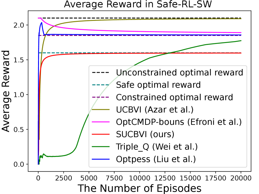


As shown in Figure 1, the rewards of SUCBVI and SRF-UCRL converge to the optimal rewards under safety constraints (denoted by "safe optimal reward"). In contrast, the rewards of UCBVI and UCRL converge to the optimal rewards without safety constraints (denoted by "unconstrained optimal reward"), and those of CMDP algorithms converge to a policy with low expected violation (denoted by "constrained optimal reward"). For Safe-RFE-SW, the expected violation of output policy of SRF-UCRL converges to zero while that of RF-UCRL does not. This corroborates the ability of SRF-UCRL in finding policies that simultaneously achieve safety and high rewards.
8 Conclusion
In this paper, we investigate a novel safe reinforcement learning problem with step-wise safety constraints. We first provide an algorithmic framework SUCBVI to achieve both regret and step-wise or gap-dependent bounded violation that is independent of . Then, we provide two lower bounds to validate the optimality of SUCBVI in both violation and regret in terms of and . Further, we extend our framework to the safe RFE with a step-wise violation and provide an algorithm SRF-UCRL that identifies a near-optimal safe policy given any reward function and guarantees violation during exploration.
References
- Achiam et al. (2017) Joshua Achiam, David Held, Aviv Tamar, and Pieter Abbeel. Constrained policy optimization. In International conference on machine learning, pp. 22–31. PMLR, 2017.
- Afsar et al. (2022) M Mehdi Afsar, Trafford Crump, and Behrouz Far. Reinforcement learning based recommender systems: A survey. ACM Computing Surveys, 55(7):1–38, 2022.
- Alshiekh et al. (2018) Mohammed Alshiekh, Roderick Bloem, Rüdiger Ehlers, Bettina Könighofer, Scott Niekum, and Ufuk Topcu. Safe reinforcement learning via shielding. In Proceedings of the AAAI Conference on Artificial Intelligence, volume 32, 2018.
- Amani et al. (2021) Sanae Amani, Christos Thrampoulidis, and Lin Yang. Safe reinforcement learning with linear function approximation. In International Conference on Machine Learning, pp. 243–253. PMLR, 2021.
- Auer et al. (2008) Peter Auer, Thomas Jaksch, and Ronald Ortner. Near-optimal regret bounds for reinforcement learning. Advances in neural information processing systems, 21, 2008.
- Azar et al. (2017) Mohammad Gheshlaghi Azar, Ian Osband, and Rémi Munos. Minimax regret bounds for reinforcement learning. In International Conference on Machine Learning, pp. 263–272. PMLR, 2017.
- Berkenkamp et al. (2017) Felix Berkenkamp, Matteo Turchetta, Angela Schoellig, and Andreas Krause. Safe model-based reinforcement learning with stability guarantees. Advances in neural information processing systems, 30, 2017.
- Bura et al. (2021) Archana Bura, Aria HasanzadeZonuzy, Dileep Kalathil, Srinivas Shakkottai, and Jean-Francois Chamberland. Safe exploration for constrained reinforcement learning with provable guarantees. arXiv preprint arXiv:2112.00885, 2021.
- Chow et al. (2018) Yinlam Chow, Ofir Nachum, Edgar Duenez-Guzman, and Mohammad Ghavamzadeh. A lyapunov-based approach to safe reinforcement learning. Advances in neural information processing systems, 31, 2018.
- Dalal et al. (2018) Gal Dalal, Krishnamurthy Dvijotham, Matej Vecerik, Todd Hester, Cosmin Paduraru, and Yuval Tassa. Safe exploration in continuous action spaces. arXiv preprint arXiv:1801.08757, 2018.
- Ding et al. (2020) Dongsheng Ding, Kaiqing Zhang, Tamer Basar, and Mihailo Jovanovic. Natural policy gradient primal-dual method for constrained markov decision processes. Advances in Neural Information Processing Systems, 33:8378–8390, 2020.
- Ding et al. (2021) Dongsheng Ding, Xiaohan Wei, Zhuoran Yang, Zhaoran Wang, and Mihailo Jovanovic. Provably efficient safe exploration via primal-dual policy optimization. In International Conference on Artificial Intelligence and Statistics, pp. 3304–3312. PMLR, 2021.
- Efroni et al. (2020) Yonathan Efroni, Shie Mannor, and Matteo Pirotta. Exploration-exploitation in constrained mdps. arXiv preprint arXiv:2003.02189, 2020.
- Hoeffding (1994) Wassily Hoeffding. Probability inequalities for sums of bounded random variables. In The collected works of Wassily Hoeffding, pp. 409–426. Springer, 1994.
- Huang et al. (2022) Ruiquan Huang, Jing Yang, and Yingbin Liang. Safe exploration incurs nearly no additional sample complexity for reward-free rl. arXiv preprint arXiv:2206.14057, 2022.
- Jin et al. (2020) Chi Jin, Akshay Krishnamurthy, Max Simchowitz, and Tiancheng Yu. Reward-free exploration for reinforcement learning. In International Conference on Machine Learning, pp. 4870–4879. PMLR, 2020.
- Kalagarla et al. (2021) Krishna C Kalagarla, Rahul Jain, and Pierluigi Nuzzo. A sample-efficient algorithm for episodic finite-horizon mdp with constraints. In Proceedings of the AAAI Conference on Artificial Intelligence, volume 35, pp. 8030–8037, 2021.
- Kaufmann et al. (2021) Emilie Kaufmann, Pierre Ménard, Omar Darwiche Domingues, Anders Jonsson, Edouard Leurent, and Michal Valko. Adaptive reward-free exploration. In Algorithmic Learning Theory, pp. 865–891. PMLR, 2021.
- Lanctot et al. (2019) Marc Lanctot, Edward Lockhart, Jean-Baptiste Lespiau, Vinicius Zambaldi, Satyaki Upadhyay, Julien Pérolat, Sriram Srinivasan, Finbarr Timbers, Karl Tuyls, Shayegan Omidshafiei, et al. Openspiel: A framework for reinforcement learning in games. arXiv preprint arXiv:1908.09453, 2019.
- Le et al. (2019) Hoang Le, Cameron Voloshin, and Yisong Yue. Batch policy learning under constraints. In International Conference on Machine Learning, pp. 3703–3712. PMLR, 2019.
- Liu et al. (2021a) Tao Liu, Ruida Zhou, Dileep Kalathil, Panganamala Kumar, and Chao Tian. Learning policies with zero or bounded constraint violation for constrained mdps. Advances in Neural Information Processing Systems, 34:17183–17193, 2021a.
- Liu et al. (2021b) Tao Liu, Ruida Zhou, Dileep Kalathil, Panganamala Kumar, and Chao Tian. Learning policies with zero or bounded constraint violation for constrained mdps. Advances in Neural Information Processing Systems, 34:17183–17193, 2021b.
- Liu et al. (2020) Yongshuai Liu, Jiaxin Ding, and Xin Liu. Ipo: Interior-point policy optimization under constraints. In Proceedings of the AAAI conference on artificial intelligence, volume 34, pp. 4940–4947, 2020.
- Ménard et al. (2021) Pierre Ménard, Omar Darwiche Domingues, Anders Jonsson, Emilie Kaufmann, Edouard Leurent, and Michal Valko. Fast active learning for pure exploration in reinforcement learning. In International Conference on Machine Learning, pp. 7599–7608. PMLR, 2021.
- Miryoosefi & Jin (2022) Sobhan Miryoosefi and Chi Jin. A simple reward-free approach to constrained reinforcement learning. In International Conference on Machine Learning, pp. 15666–15698. PMLR, 2022.
- Osband & Van Roy (2016) Ian Osband and Benjamin Van Roy. On lower bounds for regret in reinforcement learning. arXiv preprint arXiv:1608.02732, 2016.
- Qiu et al. (2020) Shuang Qiu, Xiaohan Wei, Zhuoran Yang, Jieping Ye, and Zhaoran Wang. Upper confidence primal-dual reinforcement learning for cmdp with adversarial loss. Advances in Neural Information Processing Systems, 33:15277–15287, 2020.
- Shi et al. (2023) Ming Shi, Yingbin Liang, and Ness Shroff. A near-optimal algorithm for safe reinforcement learning under instantaneous hard constraints. arXiv preprint arXiv:2302.04375, 2023.
- Simão et al. (2021) Thiago D Simão, Nils Jansen, and Matthijs TJ Spaan. Alwayssafe: Reinforcement learning without safety constraint violations during training. 2021.
- Simchowitz & Jamieson (2019) Max Simchowitz and Kevin G Jamieson. Non-asymptotic gap-dependent regret bounds for tabular mdps. Advances in Neural Information Processing Systems, 32, 2019.
- Singh et al. (2020) Rahul Singh, Abhishek Gupta, and Ness B Shroff. Learning in markov decision processes under constraints. arXiv preprint arXiv:2002.12435, 2020.
- Sootla et al. (2022) Aivar Sootla, Alexander Cowen-Rivers, Jun Wang, and Haitham Bou Ammar. Enhancing safe exploration using safety state augmentation. Advances in Neural Information Processing Systems, 35:34464–34477, 2022.
- Stooke et al. (2020) Adam Stooke, Joshua Achiam, and Pieter Abbeel. Responsive safety in reinforcement learning by pid lagrangian methods. In International Conference on Machine Learning, pp. 9133–9143. PMLR, 2020.
- Sutton & Barto (2018) Richard S Sutton and Andrew G Barto. Reinforcement learning: An introduction. MIT press, 2018.
- Tessler et al. (2018) Chen Tessler, Daniel J Mankowitz, and Shie Mannor. Reward constrained policy optimization. arXiv preprint arXiv:1805.11074, 2018.
- Thomas et al. (2021) Garrett Thomas, Yuping Luo, and Tengyu Ma. Safe reinforcement learning by imagining the near future. Advances in Neural Information Processing Systems, 34:13859–13869, 2021.
- Turchetta et al. (2020) Matteo Turchetta, Andrey Kolobov, Shital Shah, Andreas Krause, and Alekh Agarwal. Safe reinforcement learning via curriculum induction. Advances in Neural Information Processing Systems, 33:12151–12162, 2020.
- Uchibe & Doya (2007) Eiji Uchibe and Kenji Doya. Constrained reinforcement learning from intrinsic and extrinsic rewards. In 2007 IEEE 6th International Conference on Development and Learning, pp. 163–168. IEEE, 2007.
- Wachi & Sui (2020) Akifumi Wachi and Yanan Sui. Safe reinforcement learning in constrained markov decision processes. In International Conference on Machine Learning, pp. 9797–9806. PMLR, 2020.
- Wang et al. (2022) Yixuan Wang, Simon Sinong Zhan, Ruochen Jiao, Zhilu Wang, Wanxin Jin, Zhuoran Yang, Zhaoran Wang, Chao Huang, and Qi Zhu. Enforcing hard constraints with soft barriers: Safe reinforcement learning in unknown stochastic environments. arXiv preprint arXiv:2209.15090, 2022.
- Wei et al. (2022) Honghao Wei, Xin Liu, and Lei Ying. Triple-q: A model-free algorithm for constrained reinforcement learning with sublinear regret and zero constraint violation. In International Conference on Artificial Intelligence and Statistics, pp. 3274–3307. PMLR, 2022.
- Yu et al. (2022) Dongjie Yu, Haitong Ma, Shengbo Li, and Jianyu Chen. Reachability constrained reinforcement learning. In International Conference on Machine Learning, pp. 25636–25655. PMLR, 2022.
- Yu et al. (2019) Ming Yu, Zhuoran Yang, Mladen Kolar, and Zhaoran Wang. Convergent policy optimization for safe reinforcement learning. Advances in Neural Information Processing Systems, 32, 2019.
- Yu et al. (2021) Tiancheng Yu, Yi Tian, Jingzhao Zhang, and Suvrit Sra. Provably efficient algorithms for multi-objective competitive rl. In International Conference on Machine Learning, pp. 12167–12176. PMLR, 2021.
- Zhao et al. (2020) Wenshuai Zhao, Jorge Peña Queralta, and Tomi Westerlund. Sim-to-real transfer in deep reinforcement learning for robotics: a survey. In 2020 IEEE Symposium Series on Computational Intelligence (SSCI), pp. 737–744. IEEE, 2020.
Appendix
1
Appendix A Related Works
Safe RL except for CMDP-approaches
Apart from the CMDP approaches, (Yu et al. (2019); Qiu et al. (2020); Efroni et al. (2020); Ding et al. (2021); Kalagarla et al. (2021); Simão et al. (2021); Liu et al. (2021b); Bura et al. (2021); Wei et al. (2022)), there are several other ways to achieve safety in reinforcement learning. The control-based approaches (Berkenkamp et al. (2017); Chow et al. (2018); Liu et al. (2020); Wang et al. (2022)) adopt barrier functions to keep the agent away from unsafe regions and impose hard constraints. The policy-optimization style approaches are also commonly studied to solve constrained RL problems. (Uchibe & Doya (2007); Achiam et al. (2017); Tessler et al. (2018); Liu et al. (2020); Stooke et al. (2020))
There are some other papers investigating the safety of RL problems. Alshiekh et al. (2018) represents the safe state by the reactive system, and uses shielding to calculate and restrict the agent within a safe trajectory completely. The main difference between their work and our work is that we need to dynamically update the estimated safe state, while they require to know the mechanism and state to calculate the shield. Dalal et al. (2018) considers restricting the safe action by projecting the action into the closest safe actions. They achieve this goal by solving a convex optimization problem on the continuous action set. However, in their paper, they do not consider the situation where a state can have no safe actions. To be more specific, they do not consider the situation when the convex optimization problem has no solutions. Le et al. (2019) considers the decision-making problem with a pre-collected dataset. Turchetta et al. (2020) and Sootla et al. (2022) both consider cumulative cost constraints rather than step-wise constraints. The former uses a teacher for intervention to keep the agent away from the unsafe region, while the latter encourages safe exploration by augmenting a safety state to measure safety during training.
RFE with Safety
Motivated by sparse reward signals in realistic applications, reward-free exploration (RFE) has been proposed in Jin et al. (2020), and further developed in Kaufmann et al. (2021); Ménard et al. (2021). In RFE, the agent explores the environment without reward signals. After enough exploration, the reward function is given, and the agent needs to plan a near-optimal policy based on his knowledge collected in exploration. Safety is also important in RFE: We need to not only guarantee that our outputted policy is safe, but also ensure small violations during exploration.
In recent years, Huang et al. (2022) studies RFE with safety constraints. Our work differs from this work in the following aspects: (i) They allow different reward functions during exploration and after exploration, and the agent can directly know the true costs during training. In our work, the cost function is the same during and after exploration, but the agent can only observe the noisy costs of a state when she arrives at that state. (ii) They require prior knowledge of safe baseline policies, while we do not need such an assumption. (iii) They consider the zero-expected violation during exploration, while we focus on keeping small step-wise violations.
Appendix B Proofs of Main Results
B.1 Proof of Theorem 4.2
We start the proof with the confidence bound of optimistic estimation:
Lemma B.1.
With probability at least , the empirical optimistic estimation of cost function are always less than the true cost for any episode . In other words, let the event be
| (6) |
then
Proof.
Lemma B.2.
Let the event and are
Then , .
Proof.
This lemma is very standard in analysis of UCBVI algorithm. The can be derived by Bernstein’s inequality, and can be derived by Azuma-hoeffding inequality. ∎
The following lemma shows the optimistic property we discussed in the paper.
Lemma B.3.
Under the event , and for all and .
Proof.
Under the event , for all , . So . Now from our definition of , we can easily have for all step because we add the possible next state one by one into estimated set .
Now we prove the lemma by induction. When , . Assume that , then
and
Hence we complete the proof by induction. ∎
Similar to UCBVI algorithm, we prove that and are always greater than and .
Lemma B.4.
With probability at least , choosing , we will have
for any state , action , episode and the step .
Proof.
We proof this lemma by induction. First, consider , then and for all . Then our statements hold for . Now fixed an episode and assume this statement holds for . If , our proof is completed. Then assume and
where the first inequality is induction hypothesis, and the second inequality follows naturally by Chernoff-Hoeffding’s inequality. Then for
For since we know , . Then
| (7) | ||||
where Eq. (7) is because by our optimistic exploration mechanism. ∎
Regret
Now we can start to prove our main theorem.
Proof.
Having the previous analysis, our proof is similar to UCBVI algorithm. Note that the regret can be bounded by UCB:
Because the action taking by is equal to action taking at episode , we will have
where . Then
| (8) |
First, by Chernoff-Hoeffding’s bound, Second, by the standard analysis of UCBVI (Theorem 1 in UCBVI), under the event , we will have
where the first inequality holds under the event , and the second inequality is derived by , and the last inequality is because . Thus combining with Eq. (8), we can get
Denote
we have
then by recursion,
Under the event with Bernstein’s inequality, , and
| (9) |
Also, for , we can get
Then the regret will be bounded by .
Violation
Now we turn to consider the violation during the process.
First, if the agent follows the at episode , and for all step , from the definition of and , all states are safe. Since , for each state , we can have
where the first inequality from the event and the second inequality is because . Then
Then we consider the situation that for some step at episode . In this particular case, we can only bound the violation on this episode by because the future state are not in control. Fortunately, in this situation we will add at least one new state to , then , and the summation
Note that for any episode , the summation has a trivial upper bound
this situation will also appears for at most episode and leads at most extra violation.
Hence the total violation can be upper bounded by
| (10) | ||||
with probability at least . The inequality Eq. (10) is derived by Lemma 19 in Auer et al. (2008). By replacing to we can complete our proof.
Moreover, for the unsafe state set , recall that . For the state , if , we have
Thus we can get
Now denote be the set of episodes that . Now for each , denote , then our total violation can be bounded by
∎
B.2 Proof of Theorem 6.2
First, apply the same argument in the Appendix B.1, the violation during the exploration phase can be bounded by
Now we prove the Algorithm 2 will return -safe and -optimal policy. Lemma B.5 shows that bounds the estimation error for any reward function .
Lemma B.5.
For any feasible policy , step , episode and reward function , defining the estimation error as . Then, with probability at least , we have
First, we prove the Lemma B.5. We provide an lemma to show a high probability event for concentration.
Lemma B.6 (Kaufmann et al. (2021)).
Define the event as
where . Then .
By Bellman equations,
By the Pinkser’s inequality and event ,
By induction, if , for , we can have
| (11) | ||||
The second inequality is because for all , and then for . The third inequality holds by induction hypothesis, and the last inequality holds by the definition of .
Also, for other state-action pair , we can get
Hence the Lemma B.5 is true. Now we assume the algorithm terminates at episode , for any feasible policy , if we define the value function in model as , we will get
where the second inequality is because is the greedy policy with respect to and is in the feasible policy set at episode . Then for any reward function , denote the to be the optimal policy in estimated MDP . Recall that , we will have
Now we consider the expected violation. We will show that for all feasible policy , the expected violation will be upper bounded by
We first consider the event for feasible policy
Assume that the event holds, then because is the feasible policy with respect to , we have for all . Then
and under the event
| (12) |
Now define
Since , we have by recursion. The proof is similar to B.5.
Also denote
Next we prove To show this fact, we use the induction. When , . Now assume that , then
Thus by induction, we know because .
From now, we have proved that under the condition , the expected violation can be upper bounded by . Next we state that is small. Recall that , we define
and
Then by recursion, we can easily show that by .
Lemma B.7.
For all and feasible policy , we have .
Proof.
Define as
We will show We prove these two inequalities by induction. First, for , these inequalities holds. Now assume that they hold for , then
Now to prove that , we need the following lemma.
Lemma B.8.
Fixed a step and state-action pair , then with high probability at least , for any with , .
Proof.
Since we sample from for times, if , then are not sampled. The probability that are not sampled will be , where . When , the probability will be at most
Taking the union bound for all possible next state , the lemma has been proved. ∎
By the Lemma B.8, define the event as
Then . Under the event , at step and state-action pair , we have
| (13) |
This inequality is because only happens when under the event . Now we first decompose the as
The first inequality is to decompose the probability into the summation over step , and the second inequality is derived by Eq. (13). Now denote , then we can easily have by recursion. In fact, if
has the same recursive equation as . Since , by induction we can get , and then
holds directly. The Lemma B.7 has been proved.
Now we return to our main theorem. Consider the policy is one of feasible policy at episode . For each possible , denote be the probability for generating following policy and true transition kernel. If the event happens, we define the trajectory are “unsafe". Denote the set of all “unsafe" trajectories are , we have
| (14) | |||
| (15) | |||
The Eq. (14) is because implies that the event happens, and we can apply Eq. (12). The Eq. (15) is derived by the definition of and . Until now, we have proved that if the algorithm terminates, all the requirements are satisfied. Now we turn to bound the sample complexity. We first assume that
Define the average . Since the are greedy policy with respect to , we have
where . Now
Thus
where the first equality is because . Sum over , we can get
Define the pseudo-count as and the event about the pseudo-count like Kaufmann et al. (2021):
Then . The proof is provided in Kaufmann et al. (2021). Also, the Lemma 7 in Kaufmann et al. (2021) show that we can change to up to a constant.
Lemma B.9 (Kaufmann et al. (2021)).
Under the event , for any and , if is non-increasing for and is increasing, we have
The proof of Lemma B.9 can be found in Kaufmann et al. (2021). Then we can have
| (16) | ||||
| (17) |
For part , we upper bound it by
| (a) | ||||
| (18) | ||||
| (19) | ||||
where Eq. (18) is because Lemma 19 in Auer et al. (2008), Eq. (19) is derived by and Cauchy’s inequality, and the last inequality is because we assume .
Also for part ,
| (b) | ||||
| (20) | ||||
where the Eq. (20) is because the Lemma 9 in Ménard et al. (2021). Now from the upper bound of and , we can get
Recall that , by some technical transformation, performing Lemma D.1 we can get
under the event . Hence the theorem holds with probability at least , and we can prove the theorem by replacing to .
∎
B.3 Proof of Theorem 5.1
Proof.
We construct n MDP models with the same transition model but different safety cost. For each model, the states consist of a tree with degree and layer . For each state inside the tree (not a leaf), the action will lead to the th branch of the next state. For leaf nodes, they are absorbing states, and we call them . Then .

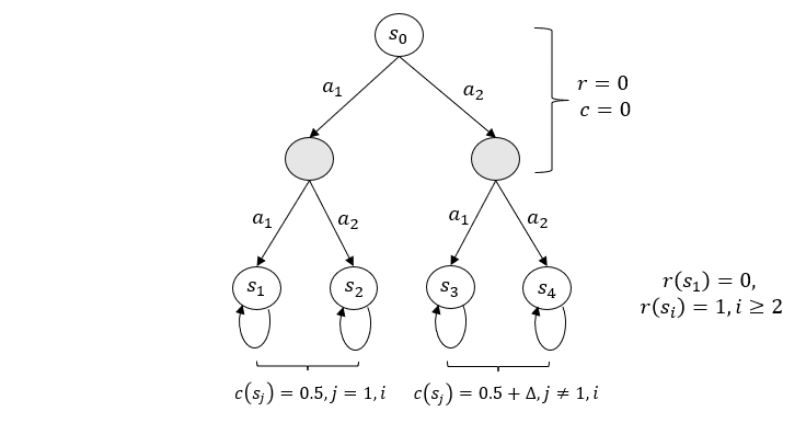
Now we first define the instance as follows: For each state inside the tree, the safety cost and reward are all 0. For leaf node, the cost function for state are . The reward function are , which implies that only state has the reward 0 and other states have reward 1. Now we define the instance . For state inside the tree, the safety cost and reward are equal to the instance . For leaf node, the cost function for state are , unchanged. Then for , the state and (and initial state ) are safe. Then the safe optimal policy is to choose at the first step. Thus the safe optimal reward is . The MDP instances are shown in Figure 2 and Figure 3.
Denote are the rest of length when we arrive at the leaf states . Let represents the regret till step episode for instance and policy , and represents the violation. For , we can have where means the times to choose the path to . Also, .
Applying Bertagnolle-Huber inequality, we have
We choose such that , then by ,
By the definition of and ,
Thus choose , (need )
If for all , then
Thus
and
where . ∎
B.4 Proof of Theorem 5.2
Proof.
Construct the MDP as follows: For each instance, the states consist of a tree with degree and layer . For each state inside the tree (not a leaf), the action will lead to the -th branch of the next state. For the leaf nodes, denote them as , where and these states will arrive at the final absorbing state and with reward and respectively. Also, the action will always lead the agent to the unique unsafe state with and for some parameter in the states except two absorbing states. For all states except the unsafe state, the safety cost is 0.
Now for the instance , the transition probability between the leaf states and absorbing states are
For instance , the transition probability are


Then if we do not consider the constraint, choosing and getting into the unsafe state is always the optimal action, then define , then the minimal gap Simchowitz & Jamieson (2019) is
Thus the regret will be at most by classical gap-dependent upper bound Simchowitz & Jamieson (2019). As we will show later, we will choose and , hence the regret will be
Now if we consider the safe threshold , the violation will be the number of time to arrive the unsafe state. Now consider any algorithm, if it achieves violation, they will arrive at unsafe state at most times. Since denote as the number of times when agent arrive at state till episode . Then . Note that each episode we will arrive at least one of once, we know , and when .
Now similar to proof of Theorem 5.1, let represents the violation with algorithm . Denote . For , we have
Also, we have
Now WLOG we have
Choose , then
Then at least one of and (assume ) have
Choose . Then assume so that
∎
Appendix C Safe Markov Games
C.1 Definitions
In this section, we provide an extension for our general framework of Safe-RL-SW. We solve the safe zero-sum two-player Markov games Yu et al. (2021).
In zero-sum two-player Markov games, there is an agent and another adversary who wants to make the agent into the unsafe region and also minimize the reward. The goal of agent is to maximize the reward and avoid the unsafe region with the existence of adversary. To be more specific, define the action space for the agent and adversary are and respectively. In each episode the agent starts at an initial state . At each step , the agent and adversary observe the state and taking action and from the strategy and simultaneously. Then the agent receive a reward and the environment transitions to the next state by the transition kernel .
One motivation of this setting is that, when a robot is in a dangerous environment, the robot should learn a completely safe policy even with the disturbance from the environment. Like the single-player MDP, we define the value function and Q-value function:
The cost function is a bounded function defined on the states , and the unsafe states are defined for some fixed threshold . Similar to the Section 4, we define the possible next states for state , step , action pair as
Hence we can define the unsafe states for step recursively as:
Then to keep safety, the agent cannot arrive at the state at the step . The safe action for the agent should avoid the unsafe region no matter what action the adversary takes.
Hence a feasible policy should keep the agent in safe state at step , and always chooses to avoid the unsafe region regardless of the adversary. Analogous to the safe RL in Section 4, assume the the optimal Bellman equation can be written as
If we denote for unsafe states , fixed an strategy for the adversary, the best response of the agent can be defined as . Similarly, a best response of the adversary given agent’s strategy can be defined as . By the minimax equality, for any step and ,
A policy pair satisfy that for all step is called a Nash Equilibrium, and the value is called the minimax value. It is known that minimax value is unique for Markov games, and the agent’s goal is make the reward closer to the minimax value.
Assume the agent and adversary executes the policy for episode , the regret is defined as
Also, the actual state-wise violation is defined as
C.2 Algorithms and Results
The main algorithm is presented in Algorithm 3. The key idea is similar to the Algorithm 1. However, in each episode we need to calculate an optimal policy by a sub-procedure “Planning". This sub-procedure calculates the Nash Equilibrium for the estimated MDP. Note that there is always a mixed Nash equilibrium strategy , and the ZERO-SUM-NASH function in “Planning" procedure calculates the Nash equilibrium for a Markov games.
In the sub-procedure “Planning", we calculate the if there exists at least one adversary action such that . In fact, the agent cannot take these actions at this time, hence by setting for these actions , the support of Nash Equilibrium policy will not contains . Otherwise, the minimax value is , and it means that is now in , then at this time the agent can chooes the action arbitrarily
Our main result are presented in the following theorem, which shows that our algorithm achieves both regret and state-wise violation.
Theorem C.1.
C.3 Proofs
Proof.
We first prove that, with probability at least , and for any episode We prove this fact by induction. Denote . The statement holds for . Suppose the bounds hold for values in the step , now we consider step .
where is all safe action for max-player at episode and step it estimated, is the true safe action, and From our algorithm, we know for all time if the confidence event always holds.
Then
The last inequality is because of the Chernoff-Hoeffding’s inequality. Thus define event
Then
Now we start to bound the regret.
Now we first assume is the best response of . Otherwise our regret can be larger. We calculate the regret by
where
The last inequality is because by Chernoff-Hoeffding’s inequality.
Now by the similar analysis in the previous section, with probability at least , the event
holds with probability at least by Bernstein’s inequality. Then for
The last inequality is because we assume is the best response of and then Now we can get
and then
By Azuma-hoeffding’s inequality, with probability at least , , and
Note that
For the violation, the argument is similar to the Theorem 4.2. During the learning process, the can appear at most times because each time the summation
will increase at least 1, and it has a upper bound . Thus it will lead to at most regret. For other situations, the total violation can be upper bounded by . Thus the final violation bound is
∎
Appendix D Technical Lemmas
D.1 Lemma D.1
Lemma D.1.
If
where , then
where ignores all the term and
Proof.
If , the lemma is trivial. Now assume , then and
Then
Case 1:
If , we can get
Subcase 1:
If by Lemma D.2, we can get .
Subcase 2:
If , we complete the proof.
Case 2:
If , we can get
Subcase 3:
If By Lemma D.2, we can get .
Subcase 4:
If , then by Lemma D.2, we can get
From the four subcases, we complete the proof of Lemma D.1.
∎
D.2 Lemma D.2
Lemma D.2.
If with , then we have .
Proof.
Define , then when , and is increasing over . Then we only need to prove there exists a constant such that
In fact, if this inequality holds, any such that should have , and then . To prove this inequality, observe that
where the third inequality is because for . So if we choose to satisfy , we have , which implies . ∎
Appendix E Detailed Analysis of Assumption 4.1
In this section, we provide a more detailed analysis of the equivalence between and the existence of feasible policy. Indeed, if the agent gets into some state at step , then any action can lead her to an unsafe next state . Recursively, any action sequence can lead the agent to unsafe states . As a result, the agent cannot avoid getting into an unsafe state. Therefore, all feasible policies must satisfy that, at any step , the probability for the agent in the state should be zero under policy .
| (21) |
Recall that
From these definitions, a feasible policy should satisfy that for any safe state . Moreover, for any safe state , there exists at least one safe action , and all possible next states satisfy . Recursively, there exists at least one feasible action sequence which satisfies that for . Hence the assumption for the existence of feasible policy can be simplified to .
Appendix F Experiment Setup
We perform each algorithm for episodes in a grid environment (Chow et al. (2018); Wei et al. (2022)) with states and actions (four directions), and report the average reward and violations across runs. In the experiment, we note that the algorithm Optpess-bouns (Efroni et al., 2020) needs to solve a linear programming with size for each episode, which is extremely slow. Thus we only compare all algorithms in a relatively small environment. In the Safe-RL-SW experiments, we choose and binary - cost function. We set the safety threshold as 0.5 for both the CMDP algorithms and the SUCBVI algorithm.
For the Safe-RFE-SW experiments, we compare our algorithm SRF-UCRL with a state-of-the-art RFE algorithm RF-UCRL (Kaufmann et al., 2021) in an MDP with 11 states and 5 actions. We choose and safety threshold of SRF-UCRL as 0.5. We run 500 episodes 100 times, and then report the average reward in each episode and cumulative step-wise violation. Also at each episode, we calculate the expected violation for the outputted policy and plot the curves. All experiments are conducted with AMD Ryzen 7 5800H with Radeon Graphics and a 16GB unified memory.