Provably End-to-end Label-noise Learning without Anchor Points

The success of modern deep learning algorithms heavily relies on large-scale accurately annotated data (Daniely & Granot, 2019; Han et al., 2020b; Xia et al., 2020; Berthon et al., 2021). However, it is often expensive or even infeasible to annotate large datasets. Therefore, cheap but less accurate annotating methods have been widely used (Xiao et al., 2015; Li et al., 2017; Han et al., 2020a; Yu et al., 2020; Zhu et al., 2021a). As a consequence, these alternatives inevitably introduce label noise. Training deep learning models on noisy data can significantly degenerate the test performance due to overfitting to the noisy labels (Arpit et al., 2017; Zhang et al., 2017; Xia et al., 2021; Wu et al., 2021).

To mitigate the negative impacts of label noise, many methods have been developed and some of them are based on a loss correction procedure. In general, these methods are statistically consistent, i.e., these methods guarantee that the classifier learned from the noisy data approaches to the optimal classifier defined on the clean risk as the size of the noisy training set increases (Liu & Tao, 2016; Scott, 2015; Natarajan et al., 2013; Goldberger & Ben-Reuven, 2017; Patrini et al., 2017; Thekumparampil et al., 2018). The idea is that the clean class-posterior $P(\boldsymbol{Y}|X=\boldsymbol{x}):=[P(Y=1|X=\boldsymbol{x}),\ldots,P(Y=C|X=\boldsymbol{x})]^{\top}$ can be inferred by utilizing the noisy class-posterior $P(\tilde{\boldsymbol{Y}}|X=\boldsymbol{x})$ and the transition matrix $\boldsymbol{T}(\boldsymbol{x})$ where $\boldsymbol{T}_{ij}(\boldsymbol{x})=P(\tilde{Y}=i|Y=j,X=\boldsymbol{x})$, i.e., $P(\boldsymbol{Y}|X=\boldsymbol{x})=[\boldsymbol{T}(\boldsymbol{x})]^{-1}P(\tilde{\boldsymbol{Y}}|X=\boldsymbol{x})$. While those methods theoretically guarantee the statistical consistency, they all heavily rely on the success of estimating transition matrices.

Generally, the transition matrix is unidentifiable without additional assumptions (Xia et al., 2019). In the literature, methods have been developed to estimate the transition matrices under the so-called anchor-point assumption: it assumes the existence of anchor points, i.e., instances belonging to a specific class with probability one (Liu & Tao, 2016). The assumption is reasonable in certain applications (Liu & Tao, 2016; Patrini et al., 2017). However, the violation of the assumption in some cases could lead to a poorly learned transition matrix and a degenerated classifier (Xia et al., 2019). This motivates the development of algorithms without exploiting anchor points (Xia et al., 2019; Liu & Guo, 2020; Xu et al., 2019; Zhu et al., 2021b). However, the performance is not theoretically guaranteed in these works.

Motivation. In this work, our interest lies in designing a consistent algorithm without anchor points, subject to class-dependent label noise, i.e., $\boldsymbol{T(\boldsymbol{x})}=\boldsymbol{T}$ for any $\boldsymbol{x}$ in the feature space. Our algorithm is based on a geometric property of the label corruption process. Given an instance $\boldsymbol{x}$, the noisy class-posterior probability $P(\tilde{\boldsymbol{Y}}|X=\boldsymbol{x}):=[P(\tilde{Y}=1|X=\boldsymbol{x}),\ldots,P(\tilde{Y}=C|X=\boldsymbol{x})]^{\top}$ can be thought of as a point in the $C$-dimensional space where $C$ is the number of classes. Since we have $P(\tilde{\boldsymbol{Y}}|X=\boldsymbol{x})=\boldsymbol{T}P(\boldsymbol{Y}|X=\boldsymbol{x})$ and $\sum_{i=1}^{C}P(Y=i|X=\boldsymbol{x})=1$, $P(\tilde{\boldsymbol{Y}}|X=\boldsymbol{x})$ is then a convex combination of the columns of $\boldsymbol{T}$. This means that the simplex $\mathrm{Sim}\{\boldsymbol{T}\}$ formed by the columns of $\boldsymbol{T}$ encloses $P(\tilde{\boldsymbol{Y}}|X=\boldsymbol{x})$ for any $\boldsymbol{x}$ (Boyd et al., 2004). Thus, the problem of identifying the transition matrix can be treated as the problem of recovering $\mathrm{Sim}\{\boldsymbol{T}\}$. However, when no assumption has been made, the problem is ill-defined as $\mathrm{Sim}\{\boldsymbol{T}\}$ is not identifiable, i.e., there exists an infinite number of simplexes enclosing $P(\tilde{\boldsymbol{Y}}|X)$, and any of them can be regarded as the true simplex $\mathrm{Sim}\{\boldsymbol{T}\}$. It is apparent that under the anchor-point assumption, $\mathrm{Sim}\{\boldsymbol{T}\}$ can be uniquely determined by exploiting anchor points whose noisy class-posterior probabilities are the vertices of $\mathrm{Sim}\{\boldsymbol{T}\}$. The goal is thus to identify the points which have the largest noisy class-posterior probabilities for each class (Liu & Tao, 2016; Patrini et al., 2017). However, if there are no anchor points, the identified points would not be the vertices of $\mathrm{Sim}\{\boldsymbol{T}\}$. In this case, existing methods cannot consistently estimate the transition matrices. To recover $\boldsymbol{T}$ without anchor points, a key observation is that, among all simplexes enclosing $P(\tilde{\boldsymbol{Y}}|X)$, $\mathrm{Sim}\{\boldsymbol{T}\}$ is the one with minimum volume. See Figure 1 for a geometric illustration. This observation motivates the development of our method which incorporates the minimum volume constraint of $\mathrm{Sim}\{\boldsymbol{T}\}$ into label-noise learning.

To this end, we propose Volume Minimization Network (VolMinNet) to consistently estimate the transition matrix and build a statistically consistent classifier. Specifically, VolMinNet consists of a classification network $\boldsymbol{h}_{\boldsymbol{\theta}}$ and a trainable transition matrix $\hat{\boldsymbol{T}}$. We simultaneously optimize $\hat{\boldsymbol{T}}$ and $\boldsymbol{h}_{\boldsymbol{\theta}}$ with two objectives: i) the discrepancy between $\hat{\boldsymbol{T}}\boldsymbol{h}_{\boldsymbol{\theta}}(\boldsymbol{x})$ and the noisy class-posterior distribution $P(\tilde{\boldsymbol{Y}}|X=\boldsymbol{x})$, ii) The volume of the simplex formed by the columns of $\hat{\boldsymbol{T}}$. The proposed framework is end-to-end, and there is no need for identifying anchor points or pseudo anchor points (i.e., instances belonging to a specific class with probability close to one) (Xia et al., 2019). Since our proposed method does not rely on any specific data points, it yields better noise robustness compared with existing methods. With a so-called sufficiently scattered assumption where the clean class-posterior distribution is far from uniform, we theoretically prove that $\hat{\boldsymbol{T}}$ will converge to the true transition matrix $\boldsymbol{T}$ while $\boldsymbol{h}_{\boldsymbol{\theta}}(\boldsymbol{x})$ converges to the clean class-posterior $P(\boldsymbol{Y}|X=\boldsymbol{x})$. We also prove that the anchor-point assumption is a special case of the sufficiently scattered assumption.

The rest of this paper is organized as follows. In Section 2, we set up the notations and review the background of label-noise learning with anchor points. In Section 3, we introduce our proposed VolMinNet. In Section 4, we present the main theoretical results. In Section 5, we briefly introduce the related works in the literature. Experimental results on both synthetic and real-world datasets are provided in Section 6. Finally, we conclude the paper in Section 7.

In this section, we review the background of label-noise learning. We follow common notational conventions in the literature of label-noise learning. $\boldsymbol{v}\in\mathbb{R}^{n}$ and $\boldsymbol{V}\in\mathbb{R}^{n\times m}$ denote a real-valued $n$-dimensional vector and a real-valued $n\times m$ matrix, respectively. Elements of a vector are denoted by a subscript (e.g., $\boldsymbol{v}_{j}$), while rows and columns of a matrix are denoted by $\boldsymbol{V}_{i,:}$ and $\boldsymbol{V}_{:,i}$ respectively. The $i$th standard basis vector in $\mathbb{R}^{C}$ is denoted by $\boldsymbol{e}_{i}$. We denote the all-ones vector by $\boldsymbol{1}$, and $\Delta^{C-1}\subset[0,1]^{C}$ is the $C$-dimensional simplex. In this work, we also make extensive use of convex analysis. Let a set $\mathcal{V}=\{\boldsymbol{v}_{1},\ldots,\boldsymbol{v}_{m}\},$ and the convex cone of $\mathcal{V}$ is denoted by $\mathrm{cone}(\mathcal{V})=\{\boldsymbol{v}|\boldsymbol{v}=\sum_{j=1}^{m}\boldsymbol{v}_{j}\alpha_{j},\;\alpha_{j}\geq 0,\;\forall j\}$. Similarly, the convex hull of $\mathcal{V}$ is defined as $\mathrm{conv}(\mathcal{V})=\{\boldsymbol{v}|\boldsymbol{v}=\sum_{j=1}^{m}\boldsymbol{v}_{j}\alpha_{j},\;\alpha_{j}\geq 0,\;\sum_{j=1}^{m}\alpha_{j}=1,\;\forall j\}$. Specially, when $\{\boldsymbol{v}_{1},\ldots,\boldsymbol{v}_{m}\}$ are affinely independent, $\mathrm{conv}(\mathcal{V})$ is also called a simplex which we denote it as $\mathrm{Sim}(\mathcal{V})$.

Let $\mathcal{D}$ be the underlying distribution generating a pair of random variables $(X,Y)\in\mathcal{X}\times\mathcal{Y},$ where $\mathcal{X}\subseteq\mathbb{R}^{d}$ is the feature space, $\mathcal{Y}=\{1,2,\ldots,C\}$ is the label space and $C$ is the number of classes. In many real-world applications, samples drawn from $\mathcal{D}$ are unavailable. Before being observed, labels of these samples are contaminated with noise and we obtain a set of corrupted data $\{(\boldsymbol{x}_{i},\tilde{y}_{i})\}_{i=1}^{n}$ where $\tilde{y}$ is the noisy label and we denote by $\tilde{\mathcal{D}}$ the distribution of the noisy random pair $(X,\tilde{Y})\in\mathcal{X}\times\mathcal{Y}$.

Given an instance $\boldsymbol{x}$ sampled from $X$, $\tilde{Y}$ is derived from the random variable $Y$ through a noise transition matrix $\boldsymbol{T}(\boldsymbol{x})\in[0,1]^{C\times C}$:

where $P(\boldsymbol{Y}|X=\boldsymbol{x})=[P(Y=1|X=\boldsymbol{x}),\ldots,P(Y=C|X=\boldsymbol{x})]^{\top}$ and $P(\tilde{\boldsymbol{Y}}|X=\boldsymbol{x})=[P(\tilde{Y}=1|X=\boldsymbol{x}),\ldots,P(\tilde{Y}=C|X=\boldsymbol{x})]^{\top}$ are the clean class-posterior probability and the noisy class-posterior probability, respectively. The $ij$-th entry of the transition matrix, i.e., $\boldsymbol{T}_{ij}(\boldsymbol{x})=P(\tilde{Y}=i|Y=j,X=\boldsymbol{x})$, represents the probability that the instance $\boldsymbol{x}$ with the clean label $Y=j$ will have a noisy label $\tilde{Y}=i$. Generally, the transition matrix is non-identifiable without any additional assumption (Xia et al., 2019). For example, we can decompose the transition matrix with $\boldsymbol{T}(\boldsymbol{x})=\boldsymbol{T}_{1}(\boldsymbol{x})\boldsymbol{T}_{2}(\boldsymbol{x})$. If we define $P^{\prime}(\boldsymbol{Y}|X=\boldsymbol{x})=\boldsymbol{T}_{2}(\boldsymbol{x})P(\boldsymbol{Y}|X=\boldsymbol{x})$, then $P(\tilde{\boldsymbol{Y}}|X=\boldsymbol{x})=\boldsymbol{T}(x)P(\boldsymbol{Y}|X=\boldsymbol{x}))=\boldsymbol{T}_{1}(\boldsymbol{x})P^{\prime}(\boldsymbol{Y}|X=\boldsymbol{x})$ are both valid. Therefore, in this paper, we study the class-dependent and instance-independent transition matrix on which the majority of existing methods focus (Han et al., 2018b, a; Patrini et al., 2017; Northcutt et al., 2017; Natarajan et al., 2013). Formally, we have:

where the transition matrix $\boldsymbol{T}$ is now independent of the instance $\boldsymbol{x}$. In this work, we also assume that the true transition matrix $\boldsymbol{T}$ is diagonally dominant¹¹1The definition of being diagonally dominant is different from the one in matrix analysis, but it has been commonly used in label-noise learning (Xu et al., 2019). Specifically, the transition matrix $\boldsymbol{T}$ is diagonally dominant if for every column of $\boldsymbol{T}$, the magnitude of the diagonal entry is larger than any non-diagonal entry, i.e., $\boldsymbol{T}_{ii}>\boldsymbol{T}_{ji}$ for any $j\neq i$. This assumption has been commonly used in the literature of label-noise learning (Patrini et al., 2017; Xia et al., 2019; Yao et al., 2020b).

As in Eq. (2), the clean class-posterior probability $P(\boldsymbol{Y}|X)$ can be inferred by using the noisy class-posterior probability $P(\tilde{\boldsymbol{Y}}|X)$ and the transition matrix $\boldsymbol{T}$ as $P(\boldsymbol{Y}|X)=\boldsymbol{T}^{-1}P(\tilde{\boldsymbol{Y}}|X)$. For this reason, the transition matrix has been widely exploited to build statistically consistent classifiers, i.e., the learned classifier will converge to the optimal classifier defined with clean risk. Specifically, the transition matrix has been used to modify loss functions to build risk-consistent estimators (Goldberger & Ben-Reuven, 2017; Patrini et al., 2017; Yu et al., 2018; Xia et al., 2019), and has been used to correct hypotheses to build classifier-consistent algorithms (Natarajan et al., 2013; Scott, 2015; Patrini et al., 2017). Thus, the successes of these consistent algorithms rely on an accurately learned transition matrix.

In recent years, considerable efforts have been invested in designing algorithms for estimating the transition matrix. These algorithms rely on a so-called anchor-point assumption which requires that there exist anchor points for each class (Liu & Tao, 2016; Xia et al., 2019).

Under the anchor-point assumption, the task of estimating the transition matrix boils down to finding anchor points for each class. For example, given anchor points $\boldsymbol{x}^{j}$, we have

Namely, the transition matrix can be obtained with the noisy class-posterior probabilities of anchor points. Assuming that we can accurately model the noisy class-posterior $P(\tilde{\boldsymbol{Y}}|X)$ given a sufficient number of noisy data, anchor points can be easily found as follows (Liu & Tao, 2016; Patrini et al., 2017):

However, when the anchor-point assumption is not satisfied, points found with Eq. (4) are no longer anchor points. Hence, the above-mentioned method can not consistently estimate the transition matrix with Eq. (3), which will lead to a statistically inconsistent classifier. This motivates us to design a statistically classifier-consistent algorithm which can consistently estimate the transition matrix without anchor points.

In this section, we propose a novel framework for label-noise learning which we call the Volume Minimization Network (VolMinNet). The proposed framework is end-to-end, and there is no need for identifying anchor points or a second stage for loss correction, resulting in better noise robustness than existing methods.

To learn the clean class-posterior $P(Y|X)$, we define a transformation $h_{\boldsymbol{\theta}}:\mathcal{X}\rightarrow\Delta^{C-1}$ where $h_{\boldsymbol{\theta}}$ is a differentiable function represented by a neural network with parameters $\boldsymbol{\theta}$. To estimate the transition matrix, we construct a trainable diagonally dominant column stochastic matrix $\hat{\boldsymbol{T}}$, i.e., $\hat{\boldsymbol{T}}\in[0,1]^{C\times C}$, $\sum_{i=1}^{C}\boldsymbol{T}_{ij}=1$ and $\boldsymbol{T}_{ii}>\boldsymbol{T}_{ji}$ for any $i\neq j$. To learn the noisy class posterior distribution from the noisy data, with some abuse of notation, we define the composition of $\hat{\boldsymbol{T}}$ and $h_{\boldsymbol{\theta}}$ as $\hat{\boldsymbol{T}}h_{\boldsymbol{\theta}}:\mathcal{X}\rightarrow\Delta^{C-1}$.

Intuitively, as explained in Section 1, if $\hat{\boldsymbol{T}}h_{\boldsymbol{\theta}}$ models $P(\tilde{\boldsymbol{Y}}|X)$ perfectly while the simplex of $\hat{\boldsymbol{T}}$ has the minimum volume, $\hat{\boldsymbol{T}}$ will converge to the true transition matrix $\boldsymbol{T}$ and $h_{\boldsymbol{\theta}}$ will converge to $P(\boldsymbol{Y}|X)$. This motivates us to propose the following criterion which corresponds to a constraint optimization problem:

where $\mathbb{T}=\{\hat{\boldsymbol{T}}\in[0,1]^{C\times C}\;|\;\sum_{i=1}^{C}\hat{\boldsymbol{T}}_{ij}=1,\;\hat{\boldsymbol{T}}_{ii}>\boldsymbol{T}_{ji},\;\forall\;i\neq j\}$ is the set of diagonally dominant column stochastic matrices. $\mathrm{vol}(\hat{\boldsymbol{T}})$ denotes a measure that is related or proportional to the volume of the simplex formed by the columns of $\hat{\boldsymbol{T}}$.

To solve criterion (5), we first note that the constraint $\hat{\boldsymbol{T}}h_{\boldsymbol{\theta}}=P(\tilde{\boldsymbol{Y}}|X)$ can be solved with expected risk minimization (Patrini et al., 2017). The risk is defined as $\tilde{R}(h_{\boldsymbol{\theta}})=\mathbb{E}_{(\boldsymbol{x},\tilde{y})\sim\tilde{D}}[\ell(\hat{\boldsymbol{T}}h_{\boldsymbol{\theta}}(\boldsymbol{x}),\tilde{y})]$, where $\ell$ is a loss function and we use the cross-entropy loss throughout this paper. We can then re-write criterion (5) as a Lagrangian under the KKT condition (Karush, 1939; Kuhn & Tucker, 2014) to obtain:

where $\beta>0$ is the KKT multiplier. In the literature, various functions for measuring the volume of the simplex have been investigated (Fu et al., 2015; Li & Bioucas-Dias, 2008; Miao & Qi, 2007). Given $\hat{\boldsymbol{T}}$ is a square matrix, a common choice is $\mathrm{vol}(\hat{\boldsymbol{T}})=\mathrm{det}(\hat{\boldsymbol{T}})$, where $\mathrm{det}$ denotes the determinant. However, this function is numerically unstable for optimization and computationally hard to deal with. Hence, we adopt another popular alternative $\log\mathrm{det}(\hat{\boldsymbol{T}})$. This function has been widely used in low-rank matrix recovery and non-negative matrix decomposition (Fazel et al., 2003; Liu et al., 2012; Fu et al., 2016). Besides, since we only have access to a set of noisy training examples $\{(\boldsymbol{x}_{i},\tilde{y}_{i})\}_{i=1}^{n}$ instead of the distribution $\tilde{\mathcal{D}}$, we employ the empirical risk for training. Formally, we propose the following objective function:

where $\lambda>0$ is a regularization coefficient that balances distribution fidelity versus volume minimization.

The problem remains how to design $\hat{\boldsymbol{T}}$ so that it is differentiable, diagonally dominant and column stochastic. Specifically, we first create a matrix $\boldsymbol{A}\in\mathbb{R}^{C\times C}$ so that diagonal elements $\boldsymbol{A}_{ii}=1$ for all $i\in\{1,2,\ldots,C\}$, and all other elements $\boldsymbol{A}_{ij}=\sigma(w_{ij})$ for all $i\neq j$ where $\sigma$ is the sigmoid function $\sigma(w)=\frac{1}{1+e^{-w}}$ and each $w_{ij}\in\mathbb{R}$ is a real-valued variable which will be updated throughout training. Then we do the normalization $\hat{\boldsymbol{T}}_{ij}=\frac{\boldsymbol{A}_{ij}}{\sum_{k=1}^{C}\boldsymbol{A}_{kj}}$ so that the sum of each column of $\hat{\boldsymbol{T}}$ is equal to one. Since the sigmoid function returns a value in the range 0 to 1, we have $\hat{\boldsymbol{T}}_{ii}>\hat{\boldsymbol{T}}_{ji}$ for all $i\neq j$. With this specially designed $\hat{\boldsymbol{T}}$, we ensure that $\hat{\boldsymbol{T}}\in\mathbb{T}$, i.e., $\hat{\boldsymbol{T}}$ is a diagonally dominant and column stochastic matrix. In addition, $\hat{\boldsymbol{T}}$ is differentiable because the sigmoid function and the normalization operation are differentiable.

With both $\hat{\boldsymbol{T}}$ and $h_{\boldsymbol{\theta}}$ being differentiable, the objective in Eq. (7) can be easily optimized with any standard gradient-based learning rule. This allows us to replace the two-stage loss correction procedure in existing works with an end-to-end learning framework. See Figure 2 for a less formal, more pedagogical explanation of our proposed learning framework.

In this section, we show that criterion (5) guarantees the consistency of the estimated transition matrix and the learned classifier under the sufficiently scattered assumption. We also show that the anchor-point assumption is a special case of the sufficiently assumption. To explain, we give a formal definition of the sufficiently scattered assumption:

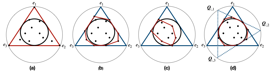
This assumption is evolved from previous works in non-negative matrix decomposition (Fu et al., 2015, 2018) with necessary modification. Intuitively, in the case of $C=3$, $\mathcal{R}$ corresponds to a “ball” tangential to the triangle formed by a permutation matrix, e.g., $\boldsymbol{I}=[\boldsymbol{e}_{1},\boldsymbol{e}_{2},\boldsymbol{e}_{3}]$. $\mathrm{cone}\{\boldsymbol{H}\}$ is the polytope inside this triangle. Columns of $\boldsymbol{Q}$ also form triangles which are rotated versions of the triangle defined by permutation matrices; facets of those triangles are also tangential to $\mathcal{R}$. Condition (1) of the sufficiently scattered assumption requires that $\mathcal{R}$ is enclosed by $\mathrm{cone}\{\boldsymbol{H}\}$, i.e., $\mathcal{R}$ is a subset of $\mathrm{cone}\{\boldsymbol{H}\}$. Condition (2) ensures that given condition (1), $\mathrm{cone}\{\boldsymbol{H}\}$ is enclosed by the triangle formed by a permutation matrix and not any other unitary matrix.

To understand the sufficiently scattered assumption and its relationship with the anchor-point assumption, we provide several examples in Figure 3. In Figure 3.(a), we show a situation where both the anchor-point assumption and sufficiently scattered assumption are satisfied. Figure 3.(b) shows a situation where the sufficiently scattered assumption is satisfied while the anchor-point assumption is violated. In Figure 3.(c) and 3.(d), both assumptions are violated. However, in Figure 3.(d), only condition (2) of the sufficiently scattered assumption is violated while both conditions of the sufficiently scattered assumption are violated in 3.(c).

The first observation is that if the anchor-point assumption is satisfied, then the sufficiently scattered assumption must hold, but not vice versa. Intuitively, if the anchor-point assumption is satisfied, then there exists a matrix $\boldsymbol{H}=[P(\boldsymbol{Y}|X=\boldsymbol{x}^{1}),\ldots,P(\boldsymbol{Y}|X=\boldsymbol{x}^{C})]=\boldsymbol{I}$ where $\boldsymbol{x}^{1},\ldots,\boldsymbol{x}^{C}$ are anchor points for different classes and $\boldsymbol{I}$ is the identity matrix. From Figure 3.(a) , it is clear that $\mathcal{R}\subseteq\mathrm{cone}\{\boldsymbol{I}\}=\mathrm{cone}\{\boldsymbol{H}\},$ and $\mathrm{cone}\{\boldsymbol{H}\}$ can only be enclosed by the convex cone of permutation matrices. This shows that the sufficiently scattered assumption is satisfied. However, from Figure 3.(b), it is clear that the sufficiently scattered assumption is satisfied but not the anchor-point assumption. Formally, we show that:

The proof of Proposition 1 is included in the supplementary material. Proposition 1 implies that the anchor-point assumption is a special case of the sufficiently scattered assumption. This means that the proposed framework can also deal with the case where the anchor-point assumption holds. Under the sufficiently scattered assumption, we get our main result:

The proof of Theorem 1 can be found in the supplementary material. Intuitively, if $P(\boldsymbol{Y}|X)$ is sufficiently scattered, the noisy class-posterior $P(\tilde{\boldsymbol{Y}}|X)$ will be sufficiently spread in the simplex formed by the columns of $\boldsymbol{T}$. Then, finding the minimum-volume data-enclosing convex hull of $P(\tilde{\boldsymbol{Y}}|X)$ recovers the ground-truth $\boldsymbol{T}$ and $P(\boldsymbol{Y}|X)$.

In this section, we review existing methods in label-noise learning. Based on the statistical consistency of the learned classifier, we divided exsisting methods for label-noise learning into two categories: heuristic algorithms and statistically consistent algorithms.

Methods in the first category focus on employing heuristics to reduce the side-effect of noisy labels. For example, many methods use a specially designed strategy to select reliable samples (Yu et al., 2019; Han et al., 2018b; Malach & Shalev-Shwartz, 2017; Ren et al., 2018; Jiang et al., 2018; Yao et al., 2020a) or correct labels (Ma et al., 2018; Kremer et al., 2018; Tanaka et al., 2018; Reed et al., 2015). Although those methods empirically work well, there is not any theoretical guarantee on the consistency of the learned classifiers from all these methods.

Statistically consistent algorithms are primarily developed based on a loss correction procedure (Liu & Tao, 2016; Patrini et al., 2017; Zhang & Sabuncu, 2018). For these methods, the noise transition matrix plays a key role in building consistent classifiers. For example, Patrini et al.(2017) leveraged a two-stage training procedure of first estimating the noise transition matrix and then use it to modify the loss to ensure risk consistency. These works rely on anchor points or instances belonging to a specific class with probability one or approximately one. When there are no anchor points in datasets or data distributions, all the aforementioned methods cannot guarantee the statistical consistency. Another approach is to jointly learn the noise transition matrix and classifier. For instance, on top of the softmax layer of the classification network (Goldberger & Ben-Reuven, 2017), a constrained linear layer or a nonlinear softmax layer is added to model the noise transition matrix (Sukhbaatar et al., 2015). Zhang et al. (2021) concurrently propose a one-step method for the label-noise learning problem and a derivative-free method for estimating the transition matrix. Specifically, their method uses a total variation regularization term to prevent the overconfidence problem of the neural network, which leads to a more accurate noisy class-posterior. However, the anchor-point assumption is still needed for their method. Based on different motivations, assumptions and learning objectives, their method achieves different theoretical results compared with our proposed method. Learning with noisy labels are also closely related to learning with complementary labels where instead of noisy labels, only compelementary labels are given for training (Yu et al., 2018; Chou et al., 2020; Feng et al., 2020).

Recently, some methods exploiting semi-supervised learning techniques have been proposed to solve the label-noise learning problem like SELF (Nguyen et al., 2019) and DivideMix (Li et al., 2019). These methods are aggregations of multiple techniques such as augmentations and multiple networks. Noise robustness is significantly improved with these methods. However, these methods are sensitive to the choice of hyperparameters and changes in data and noise types would generate degenerated classifiers. In addition, the computational cost of these methods increases significantly compared with previous methods.

In this section, we verify the robustness of the proposed volume minimization network (VolMinNet) from two folds: the estimation error of the transition matrix and the classification accuracy.

Datasets We evaluate the proposed method on three synthetic noisy datasets, i.e., MNIST, CIFAR-10 and CIFAR-100 and one real-world noisy dataset, i.e., clothing1M. We leave out 10% of the training examples as the validation set. The three synthetic datasets contain clean data. We corrupted the training and validation sets manually according to transition matrices. Specifically, we conduct experiments with two commonly used types of noise: (1) Symmetry flipping (Patrini et al., 2017); (2) Pair flipping (Han et al., 2018b). We report both the classification accuracy on the test set and the estimation error between the estimated transition matrix $\hat{\boldsymbol{T}}$ and the true transition matrix $\boldsymbol{T}$. All experiments are repeated five times on all datasets. Following T-Revision (Xia et al., 2019), we also conducted experiments on datasets where possible anchor points are removed from the datasets. The details and more experimental results can be found in the Supplementary Material.

Clothing1M is a real-world noisy dataset which consists of $1\mathrm{M}$ images with real-world noisy labels. Existing methods like Forward (Patrini et al., 2017) and T-revision (Xia et al., 2019) use the additional 50k clean training data to help initialize the transition matrix and validate on 14k clean validation data. Here we use another setting which is also commonly used in the literature (Xia et al., 2020). We only exploit the $1\mathrm{M}$ data for both transition matrix estimation and classification training. Specifically, we leave out $10\%$ of the noisy training examples as a noisy validation set for model selection. We think this setting is more natural considering that it does not require any clean data. All results of baseline methods are quoted from PTD (Xia et al., 2020) as we have the same setting.

Network structure and optimization For a fair comparison, we implement all methods with default parameters by PyTorch on Tesla V100-SXM2. For MNIST, we use a LeNet-5 network. SGD is used to train the classification network $h_{\boldsymbol{\theta}}$ with batch size $128$, momentum $0.9$, weight decay $10^{−3}$ and a learning rate $10^{-2}$. Adam with default parameters is used to train the transition matrix $\hat{\boldsymbol{T}}$. The algorithm is run for $60$ epoch. For CIFAR10, we use a ResNet-18 network. SGD is used to train both the classification network $h_{\boldsymbol{\theta}}$ and the transition matrix $\hat{\boldsymbol{T}}$ with batch size $128$, momentum $0.9$, weight decay $10^{−3}$ and an initial learning rate $10^{-2}$. The algorithm is run for $150$ epoch and the learning rate is divided by $10$ after the $30$th and $60$th epoch. For CIFAR100, we use a ResNet-32 network. SGD is used to train the classification network $h_{\boldsymbol{\theta}}$ with batch size $128$, momentum $0.9$, weight decay $10^{−3}$ and an initial learning rate $10^{-2}$. Adam with default parameters is used to train the transition matrix $\hat{\boldsymbol{T}}$. The algorithm is run for $150$ epoch and the learning rate is divided by $10$ after the $30$th and $60$th epoch. For CIFAR-10 and CIFAR-100, we perform data augmentation by horizontal random flips and $32\times 32$ random crops after padding 4 pixels on each side. For clothing1M, we use a ResNet-50 pre-trained on ImageNet. We only use the 1M noisy data to train and validate the network. For the optimization, SGD is used train both the classification network $h_{\boldsymbol{\theta}}$ and the transition matrix $\hat{\boldsymbol{T}}$ with momentum 0.9, weight decay $10^{−3}$, batch size 32, and run with learning rates $2\times 10^{−3}$ and $2\times 10^{−5}$ for 5 epochs each. For each epoch, we ensure the noisy labels for each class are balanced with undersampling. Throughout all experiments, we fixed $\lambda=10^{-4}$ and the trainable weights $w$ of $\hat{\boldsymbol{T}}$ are initialized with $ln\frac{1}{C-2}$ (roughly -2 for MNIST and CIFAR10, -4.5 for CIFAR100 and -2.5 for clothing1M).

In this paper, we considered the problem of label-noise learning without anchor points. We relax the anchor-point assumption with our proposed VolMinNet. The consistency of the estimated transition matrix and the learned classifier are theoretically proved under the sufficiently scattered assumption. Experimental results have demonstrated the robustness of the proposed VolMinNet. Future work should focus on improving the estimation of the noisy class posterior which we believe is the bottleneck of our method.

XL was supported by an Australian Government RTP Scholarship. TL was supported by Australian Research Council Project DE-190101473. BH was supported by the RGC Early Career Scheme No. 22200720, NSFC Young Scientists Fund No. 62006202 and HKBU CSD Departmental Incentive Grant. GN and MS were supported by JST AIP Acceleration Research Grant Number JPMJCR20U3, Japan. MS was also supported by Institute for AI and Beyond, UTokyo. Authors also thank for the help from Dr. Alan Blair, Kevin Lam, Yivan Zhang and members of the Trustworthy Machine Learning Lab at the University of Sydney.

References

- Arpit et al. (2017) Arpit, D., Jastrzębski, S., Ballas, N., Krueger, D., Bengio, E., Kanwal, M. S., Maharaj, T., Fischer, A., Courville, A., Bengio, Y., et al. A closer look at memorization in deep networks. In ICML, pp. 233–242, 2017.
- Berthon et al. (2021) Berthon, A., Han, B., Niu, G., Liu, T., and Sugiyama, M. Confidence scores make instance-dependent label-noise learning possible. In ICML, 2021.
- Boyd et al. (2004) Boyd, S., Boyd, S. P., and Vandenberghe, L. Convex optimization. Cambridge university press, 2004.
- Chou et al. (2020) Chou, Y.-T., Niu, G., Lin, H.-T., and Sugiyama, M. Unbiased risk estimators can mislead: A case study of learning with complementary labels. In ICML, pp. 1929–1938. PMLR, 2020.
- Daniely & Granot (2019) Daniely, A. and Granot, E. Generalization bounds for neural networks via approximate description length. In NeurIPS, pp. 13008–13016, 2019.
- Fazel et al. (2003) Fazel, M., Hindi, H., and Boyd, S. P. Log-det heuristic for matrix rank minimization with applications to hankel and euclidean distance matrices. In ACC, pp. 2156–2162, 2003.
- Feng et al. (2020) Feng, L., Kaneko, T., Han, B., Niu, G., An, B., and Sugiyama, M. Learning with multiple complementary labels. In ICML, pp. 3072–3081. PMLR, 2020.
- Fu et al. (2015) Fu, X., Ma, W.-K., Huang, K., and Sidiropoulos, N. D. Blind separation of quasi-stationary sources: Exploiting convex geometry in covariance domain. IEEE Transactions on Signal Processing, 63(9):2306–2320, 2015.
- Fu et al. (2016) Fu, X., Huang, K., Yang, B., Ma, W.-K., and Sidiropoulos, N. D. Robust volume minimization-based matrix factorization for remote sensing and document clustering. IEEE Transactions on Signal Processing, 64(23):6254–6268, 2016.
- Fu et al. (2018) Fu, X., Huang, K., and Sidiropoulos, N. D. On identifiability of nonnegative matrix factorization. IEEE Signal Processing Letters, 25(3):328–332, 2018.
- Goldberger & Ben-Reuven (2017) Goldberger, J. and Ben-Reuven, E. Training deep neural-networks using a noise adaptation layer. In ICLR, 2017.
- Han et al. (2018a) Han, B., Yao, J., Niu, G., Zhou, M., Tsang, I., Zhang, Y., and Sugiyama, M. Masking: A new perspective of noisy supervision. In NeurIPS, pp. 5836–5846, 2018a.
- Han et al. (2018b) Han, B., Yao, Q., Yu, X., Niu, G., Xu, M., Hu, W., Tsang, I., and Sugiyama, M. Co-teaching: Robust training of deep neural networks with extremely noisy labels. In NeurIPS, pp. 8527–8537, 2018b.
- Han et al. (2020a) Han, B., Niu, G., Yu, X., Yao, Q., Xu, M., Tsang, I., and Sugiyama, M. Sigua: Forgetting may make learning with noisy labels more robust. In ICML, pp. 4006–4016. PMLR, 2020a.
- Han et al. (2020b) Han, B., Yao, Q., Liu, T., Niu, G., Tsang, I. W., Kwok, J. T., and Sugiyama, M. A survey of label-noise representation learning: Past, present and future, 2020b.
- Jiang et al. (2018) Jiang, L., Zhou, Z., Leung, T., Li, L.-J., and Fei-Fei, L. MentorNet: Learning data-driven curriculum for very deep neural networks on corrupted labels. In ICML, pp. 2309–2318, 2018.
- Karush (1939) Karush, W. Minima of functions of several variables with inequalities as side constraints. M. Sc. Dissertation. Dept. of Mathematics, Univ. of Chicago, 1939.
- Kremer et al. (2018) Kremer, J., Sha, F., and Igel, C. Robust active label correction. In AISTATS, pp. 308–316, 2018.
- Kuhn & Tucker (2014) Kuhn, H. W. and Tucker, A. W. Nonlinear programming. In Traces and emergence of nonlinear programming, pp. 247–258. Springer, 2014.
- Li & Bioucas-Dias (2008) Li, J. and Bioucas-Dias, J. M. Minimum volume simplex analysis: A fast algorithm to unmix hyperspectral data. In IGARSS, pp. III–250, 2008.
- Li et al. (2019) Li, J., Socher, R., and Hoi, S. C. Dividemix: Learning with noisy labels as semi-supervised learning. In ICLR, 2019.
- Li et al. (2017) Li, W., Wang, L., Li, W., Agustsson, E., and Van Gool, L. Webvision database: Visual learning and understanding from web data. arXiv preprint arXiv:1708.02862, 2017.
- Liu et al. (2012) Liu, G., Lin, Z., Yan, S., Sun, J., Yu, Y., and Ma, Y. Robust recovery of subspace structures by low-rank representation. IEEE transactions on pattern analysis and machine intelligence, 35(1):171–184, 2012.
- Liu & Tao (2016) Liu, T. and Tao, D. Classification with noisy labels by importance reweighting. IEEE Transactions on pattern analysis and machine intelligence, 38(3):447–461, 2016.
- Liu & Guo (2020) Liu, Y. and Guo, H. Peer loss functions: Learning from noisy labels without knowing noise rates. In ICML, pp. 6226–6236. PMLR, 2020.
- Ma et al. (2018) Ma, X., Wang, Y., Houle, M. E., Zhou, S., Erfani, S. M., Xia, S.-T., Wijewickrema, S., and Bailey, J. Dimensionality-driven learning with noisy labels. In ICML, pp. 3361–3370, 2018.
- Malach & Shalev-Shwartz (2017) Malach, E. and Shalev-Shwartz, S. Decoupling" when to update" from" how to update". In NeurIPS, pp. 960–970, 2017.
- Miao & Qi (2007) Miao, L. and Qi, H. Endmember extraction from highly mixed data using minimum volume constrained nonnegative matrix factorization. IEEE Transactions on Geoscience and Remote Sensing, 45(3):765–777, 2007.
- Natarajan et al. (2013) Natarajan, N., Dhillon, I. S., Ravikumar, P. K., and Tewari, A. Learning with noisy labels. In NeurIPS, pp. 1196–1204, 2013.
- Nguyen et al. (2019) Nguyen, D. T., Mummadi, C. K., Ngo, T. P. N., Nguyen, T. H. P., Beggel, L., and Brox, T. Self: Learning to filter noisy labels with self-ensembling. In ICLR, 2019.
- Northcutt et al. (2017) Northcutt, C. G., Wu, T., and Chuang, I. L. Learning with confident examples: Rank pruning for robust classification with noisy labels. In UAI, 2017.
- Patrini et al. (2017) Patrini, G., Rozza, A., Krishna Menon, A., Nock, R., and Qu, L. Making deep neural networks robust to label noise: A loss correction approach. In CVPR, pp. 1944–1952, 2017.
- Reed et al. (2015) Reed, S. E., Lee, H., Anguelov, D., Szegedy, C., Erhan, D., and Rabinovich, A. Training deep neural networks on noisy labels with bootstrapping. In ICLR, Workshop Track Proceedings, 2015.
- Ren et al. (2018) Ren, M., Zeng, W., Yang, B., and Urtasun, R. Learning to reweight examples for robust deep learning. In ICML, pp. 4331–4340, 2018.
- Scott (2015) Scott, C. A rate of convergence for mixture proportion estimation, with application to learning from noisy labels. In AISTATS, pp. 838–846, 2015.
- Sukhbaatar et al. (2015) Sukhbaatar, S., Estrach, J. B., Paluri, M., Bourdev, L., and Fergus, R. Training convolutional networks with noisy labels. In ICLR, 2015.
- Tanaka et al. (2018) Tanaka, D., Ikami, D., Yamasaki, T., and Aizawa, K. Joint optimization framework for learning with noisy labels. In CVPR, pp. 5552–5560, 2018.
- Thekumparampil et al. (2018) Thekumparampil, K. K., Khetan, A., Lin, Z., and Oh, S. Robustness of conditional gans to noisy labels. In NeurIPS, pp. 10271–10282, 2018.
- Wu et al. (2021) Wu, S., Xia, X., Liu, T., Han, B., Gong, M., Wang, N., Liu, H., and Niu, G. Class2simi: A new perspective on learning with label noise. In ICML. PMLR, 2021.
- Xia et al. (2019) Xia, X., Liu, T., Wang, N., Han, B., Gong, C., Niu, G., and Sugiyama, M. Are anchor points really indispensable in label-noise learning? In NeurIPS, pp. 6835–6846, 2019.
- Xia et al. (2020) Xia, X., Liu, T., Han, B., Wang, N., Gong, M., Liu, H., Niu, G., Tao, D., and Sugiyama, M. Part-dependent label noise: Towards instance-dependent label noise. NerurIPS, 2020.
- Xia et al. (2021) Xia, X., Liu, T., Han, B., Gong, C., Wang, N., Ge, Z., and Chang, Y. Robust early-learning: Hindering the memorization of noisy labels. In ICLR, 2021.
- Xiao et al. (2015) Xiao, T., Xia, T., Yang, Y., Huang, C., and Wang, X. Learning from massive noisy labeled data for image classification. In CVPR, pp. 2691–2699, 2015.
- Xu et al. (2019) Xu, Y., Cao, P., Kong, Y., and Wang, Y. L_dmi: A novel information-theoretic loss function for training deep nets robust to label noise. In NeurIPS, pp. 6222–6233, 2019.
- Yao et al. (2020a) Yao, Q., Yang, H., Han, B., Niu, G., and Kwok, J. T.-Y. Searching to exploit memorization effect in learning with noisy labels. In ICML, pp. 10789–10798. PMLR, 2020a.
- Yao et al. (2020b) Yao, Y., Liu, T., Han, B., Gong, M., Deng, J., Niu, G., and Sugiyama, M. Dual t: Reducing estimation error for transition matrix in label-noise learning. In NeurIPS, 2020b.
- Yu et al. (2018) Yu, X., Liu, T., Gong, M., and Tao, D. Learning with biased complementary labels. In ECCV, pp. 68–83, 2018.
- Yu et al. (2019) Yu, X., Han, B., Yao, J., Niu, G., Tsang, I., and Sugiyama, M. How does disagreement help generalization against label corruption? In ICML, pp. 7164–7173, 2019.
- Yu et al. (2020) Yu, X., Liu, T., Gong, M., Zhang, K., Batmanghelich, K., and Tao, D. Label-noise robust domain adaptation. In ICML, pp. 10913–10924. PMLR, 2020.
- Zhang et al. (2017) Zhang, C., Bengio, S., Hardt, M., Recht, B., and Vinyals, O. Understanding deep learning requires rethinking generalization. In ICLR, 2017.
- Zhang et al. (2021) Zhang, Y., Niu, G., and Sugiyama, M. Learning noise transition matrix from only noisy labels via total variation regularization. In ICML, 2021.
- Zhang & Sabuncu (2018) Zhang, Z. and Sabuncu, M. Generalized cross entropy loss for training deep neural networks with noisy labels. In NeurIPS, pp. 8778–8788, 2018.
- Zhu et al. (2021a) Zhu, Z., Liu, T., and Liu, Y. A second-order approach to learning with instance-dependent label noise. In CVPR, 2021a.
- Zhu et al. (2021b) Zhu, Z., Song, Y., and Liu, Y. Clusterability as an alternative to anchor points when learning with noisy labels. In ICML, 2021b.
Appendix A Appendix
A.1 Proof of Proposition 1
To prove proposition 1, we first show that the anchor-point assumption is a sufficient condition for the sufficiently scattered assumption. In other words, we need to show that if the anchor-point assumption is satisfied, then two conditions of the sufficiently scattered assumption must hold.
We start with condition (2) of the sufficiently scattered assumption. We need to show that if the anchor-point assumption is hold, then there exists a set such that the matrix satisfies that , for any unitary matrix that is not a permutation matrix.
Since the anchor-point assumption is satisfied, then there exists a matrix where are anchor points for each class. From the definition of anchor points, we have . This implies that