20cm(1cm,1cm) Accepted by European Physical Journal C, the publication is available at Link
Prospect for measurement of the CP-violating phase in the channel at a future factory
Abstract
The CP-violating phase , the decay width (), and the decay width difference () are sensitive probes to new physics and can constrain the heavy quark expansion theory. The potential for the measurement at future factories is studied in this manuscript. It is found that operating at Tera- mode, the expected precision can reach: , and . The precision of is 40% larger than the expected precision with the LHCb experiment at HL-LHC. If operating at 10-Tera- mode, the precision of can be measured at 45% of the precision obtained from the LHCb experiment at HL-LHC. However, the measurement of and cannot benefit from the excellent time resolution and tagging power of the future -factories. Only operating at 10-Tera- mode can the and reach an 18% larger precision than the precision expected to be obtained from LHCb at HL-LHC. The control of penguin contamination at the future Z-factories is also discussed.
1 Introduction
In the Standard Model (SM), CP violation is attributed to the Cabibbo-Kobayashi-Maskawa (CKM) matrix. The CP-violating phase, denoted as , emerges from the interference between the direct decay amplitude of the meson and the amplitude of the meson decaying after – oscillation. In the SM, when subleading contributions are neglected, the phase is predicted to be , where is defined as , represented by the elements of the CKM matrix. However, when accounting for the penguin diagram’s contribution, the phase is modified by a shift , resulting in . The current SM prediction for the phase is , according to the CKMFitter group [1], and from the UTfit Collaboration [2]. The global average in experiments stands at [3], with the uncertainty being approximately 20 times larger than that of the SM prediction. Accurate measurement of serves as a critical test for the Standard Model.
The meson exists in two mass eigenstates, known as the light (L) and heavy (H) states, each with distinct decay widths, denoted as and , respectively. Measurements of the decay width difference, , and the average decay width, , hold significant theoretical interest. The Heavy Quark Expansion (HQE) [4] theory provides a robust framework for calculating various observables related to -hadrons. Accurate measurements of and serve as critical tests for the validity of the HQE theory.
After the Higgs boson discovery in 2012, the Circular Electron-Positron Collider (CEPC) and the Future Circular Collider (FCC-ee) were proposed. These colliders are designed not only as Higgs factories but also to operate at the pole configuration. In this mode, they are projected to produce between and bosons over a decade. Consequently, from the decay of these bosons, approximately pairs are expected to be generated. Thus, the future -factories are proposed to serve concurrently as -factories. Using a time projection chamber or a wire chamber as the main tracking detector, the detectors at the CEPC and FCC-ee offer excellent particle identification, highly accurate track and vertex reconstruction, and extensive geometric acceptance, which are all important in heavy flavor physics study. These capabilities position the future -factories as excellent experiments for advancing heavy flavor physics research.
This paper explores the expected measurement precision at future -factories, extrapolating from measurements from current operating experiments. The extrapolation process is carried out as follows: First, we list all important factors influencing measurement precision, including the statistical data size and detector performances. We then figure out the mathematical relationship determining how these factors influence measurement precision. Subsequently, for each of these factors, we assess their performance at future -factories. Finally, we compare the performances of these factors between the future colliders and the current existing experiments. The expected precision of the interested parameters at the future colliders is then computed by applying the mathematical relationship, using inputs from the statistical data size and detector performances.
1.1 Measurement of (, ) in experiments
The CP-violating phase , decay width , and the width difference between the heavier and lighter meson eigenstates have been thoroughly investigated in experiments conducted by ATLAS [5, 6], CDF [7], CMS [8, 9], D0 [10], and LHCb [11, 12, 13, 14, 15, 16]. The decay channel is particularly notable due to its sizeable branching fraction and the final state consisting entirely of charged tracks. This decay channel benefits from the narrow decay widths of the and particles, effectively suppressing the combinatorial background. It stands as the most prominent channel for measuring , and it also allows for the concurrent extraction of and .
The time and angular distribution of is a sum of ten terms corresponding to the three polarization amplitudes and the non-resonant S-wave, together with their interference terms:
| (1) |
where
and is the amplitude function.
In the formulation of , the term represents the mass difference between the mass eigenstates, while denotes the amplitude of the component at . The phase is encapsulated within the parameters , and . For an in-depth explanation of these parameters, one can refer to the LHCb publication [12]. The values of , , and could be obtained by fitting the time and angular distributions of decay events.
Additionally, when determining , and , parameters such as can also be simultaneously derived from this fitting. However, the precision of these parameters is beyond the scope of this work and will not be discussed here.
2 Estimation of precision on the future factory
The statistical precision of the measurement, denoted by , is directly proportional to the inverse square root of the effective signal sample size. This effective sample size is, in turn, dependent on the number of pairs () produced by the collider. Additionally, the effective signal sample size is proportional to the detector’s acceptance and efficiency .
Identifying the initial flavor, either or , is essential for extracting parameters from Eq. (1). This procedure is known as flavor tagging. The tagging efficiency, denoted by , represents the fraction of particles that the tagging algorithm can identify, regardless of whether the identification is correct or not. The mistagging rate, denoted by , represents the proportion of incorrectly identified particles among those that are identified. The is expressed as:
where is the number of events correctly tagged, and is the number of events incorrectly tagged. The difficulty in accurately identifying the initial flavor, along with the rate of misidentification, reduces the precision of extracting parameters from the fit. Consequently, the effective sample size is reduced by a factor known as the tagging power, represented by , in comparison to an ideal scenario of perfect tagging, where
Another important factor that affects the precision of measurements is the resolution of the proper decay time measurement, donated as . This resolution impacts the precision of measurements in the format of , where is the mass difference of the two eigenstates, as detailed in Appendix.
A scaling factor, which is proportional to the , can be established as follows:
| (2) |
This scaling factor allows us to estimate the expected precision of in future -factories with
| (3) |
where FE denotes a future experiment and EE denotes an existing experiment.
In this study, the precision and scaling factor for the existing experiment are estimated from the LHCb studies [12]. For the LHCb measurement, the number of extracted signals is = . The flavor tagging power is . The decay time resolution is measured as . The precision of is measured to be . Consequently, the scale factor is calculated to be , and the ratio is .
The scaling factor for the future -factory is estimated through a Monte Carlo study. The details of the estimation will be elaborated in the subsequent sections.
The scaling factor for experiments conducted at the High-Luminosity LHC (HL-LHC) is also calculated for comparison. It is assumed that there will be no significant changes in the detector’s acceptance, efficiency, tagging power, or decay time resolution at the HL-LHC. The scaling factor is determined by scaling for the increase in luminosity. At the HL-LHC, the anticipated luminosity is , compared to the current measurement of at LHCb.
Therefore, the scaling factor is
. Based on this, the expected precision for is calculated to be
. This estimate suggests a slightly more promising outcome than the one presented in Ref.
[17], which is .
The estimation presented in Ref. [17] is based on a projection from Ref [11].
The discrepancy between the two estimates could be attributed to the improvement of flavor tagging employed in the study of Ref. [12], which marks an advancement over the methodologies used in the earlier study, Ref. [11].
The expected precision for the parameters and is estimated in a similar manner as the estimation of measurement precision. These parameters are primarily influenced by the shape of the exponential decay and are less impacted by oscillatory behavior. Consequently, when the decay time resolution is small, they are not as sensitive to the tagging power and the resolution of the proper decay time, which distinguishes them from measurements. This assertion is further confirmed by simulations, as detailed in Appendix. The variable
| (4) |
is introduced as the scaling factor for and . The scaling factor for LHCb is , estimated from Ref. [12].
2.1 CEPC and the baseline detector
The CEPC and the baseline detector (CEPC-v4) [18] are taken as an example to study the precision of , and . As a baseline, the CEPC is assumed to run in the Tera- mode, i.e., produces bosons during its lifetime. The CEPC baseline detector consists of a vertex system, a silicon inner tracker, a TPC, a silicon external tracker, an electromagnetic calorimeter, a hadron calorimeter, a solenoid of 3 Tesla, and a Return Yoke.
2.2 Monte Carlo sample and reconstruction
A Monte Carlo signal sample is generated to analyze the geometric acceptance and the reconstruction efficiency of the decay. Additionally, this sample is also used for the examination of the proper decay time resolution for the , which has a direct correlation with the spatial resolution at the decay vertex.
Using the WHIZARD [19] generator, roughly 6000 events of are simulated. The particles are then forced to decay through the process using PYTHIA 8 [20], with a uniform distribution in phase space.
The simulation of particle transport within the detector utilizes MokkaC, the simulation software for the CEPC study, based on the GEANT 4 [21]. Based on Monte Carlo truth data, the reconstructed particles are categorized into hadrons, muons, and electrons.
The candidates are reconstructed from every pairing of a positively charged muon with a negatively charged muon. They are then selected based on the invariant mass window, ranging from to . The candidates are reconstructed from every possible combination of a positively charged kaon and a negatively charged kaon. The candidates are selected within the mass window from to . The meson is reconstructed by combining all pairs of and candidates identified in the preceding steps. The four-momentum of the meson is determined using the four-momentum of the and , ensuring conservation of energy and momentum. They are selected within a mass window ranging from to . Following the reconstruction of the meson, a decay vertex is constructed using the tracks associated with the .
As the CEPC was initially designed as a Higgs factory, the secondary vertex reconstruction algorithm and the flavor tagging algorithm are not in the standard CEPC software chain. A vertex reconstruction procedure and a simple flavor tagging algorithm were specially implemented for this study, which will be described in Sect. 2.5.
An additional sample of is generated to show that a low background level is achievable through appropriate event selection criteria for the measurement. The detector simulation and event reconstruction processes are consistent with those applied to the signal sample.
2.3 Statistics and acceptance efficiency
Assuming that all events can be selected with high purity, the background events in this work are the events that do not contain signal. The branching fraction of hadronized to is 10% [22]. The branching ratio of is . And the branching ratio of , are and respectively [22]. If the background is not suppressed by any event selection criteria, the number of background events is times larger than the number of signal events. Applying the invariant mass selection criteria described in Sect. 2.2 to the background sample, the probability of reconstructing a fake candidate from a event is . Therefore, after the event selection, background statistics are of the same magnitude as the signal statistics.
The combinatorial background events that pass the invariant mass selection criteria are further suppressed by using vertex information. In the background events, the fake candidates come from four arbitrarily combined tracks, two of which are lepton tracks and two of which are hadron tracks. The lepton usually has a large impact parameter, and the hadron has a small one. It is difficult to reconstruct a high-quality vertex with arbitrarily combined tracks. The is used to measure the quality of the vertex reconstruction, where
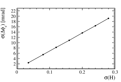
The in the formula represents the distance from the reconstructed vertex to the track in the plane perpendicular to the beam direction. The distributions of the signal and background are shown in Fig. 1. The vertex of signal is usually very small. And the of background is distributed over an extensive range. With a very loose cut at , of the signals are selected and of the backgrounds are discarded.
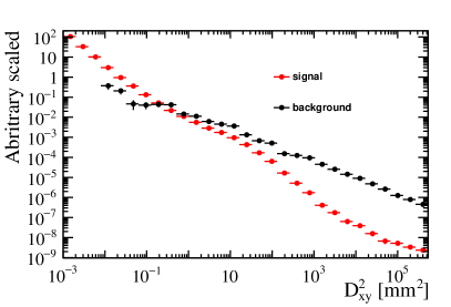
By employing a combination of invariant mass and vertex cut, the acceptance efficiency of the signal is 75%, while the background is maintained at 1% of the signal level.
Due to potential particle misidentification, a small peaking background may be present in the signal region. Implementing a strict threshold on the hadron ID can reduce this peaking background; however, it would also result in diminished efficiency. This loss of efficiency is not considered in the present analysis due to the excellent PID performances of the CEPC.
At CEPC, the electron tracking performance is as good as that of muon tracking. The could be reconstructed via the channel as well. Consequently, the total effective sample size is considered to be roughly twice as much as when only the decay channel is considered.
2.4 Flavor tagging
2.4.1 Flavor tagging algorithm
A simple algorithm is developed to identify the initial flavor of the particle. The idea of the algorithm is as follows:
The () quarks are predominantly produced in pairs that fly in the opposite directions because of the momentum conservation. The flavor of the opposite -quark can be used to determine the initial flavor of the interested . To judge the flavor of this opposite -quark, we take a lepton and a charged kaon with maximum momentum in the opposite direction of the . The lepton and kaon charge provides the flavor of the opposite -quark. Furthermore, when the quark is hadronized to a meson, another quark is spontaneously created, which has the chance to become a charged kaon, flying in a similar direction to the . Based on this kaon, one can identify the flavor of the particle. The algorithm takes the leading particles (particles with the largest momentum projected onto the direction of the ). If these particles provide different determinants for the flavor, the algorithm says that it cannot identify the flavor. The kaons and the muons from the decay are excluded from the consideration in the above algorithms.
2.4.2 Flavor tagging power
The algorithm is applied to a Monte Carlo truth-level simulation, assuming perfect particle identification. The probability of finding a charged kaon at the near side (the angle between the momentum of the two particles is less than ) of the is . Within the events with near-side kaons, () of the leading kaons are () if a rather than is produced. The significant difference between the abundance of and makes the nearside kaon a powerful distinguish observable to identify the initial flavor of the meson. At the opposite side (the angle between the momentum of the two particles is larger than ), the probability of finding a charged kaon is %. The percentage of the is , while the percentage of the is for the leading kaons. The probability of finding an electron or muon at the opposite side of is , where the probability of the leading particle to be an electron, positron, muon, or anti-muon is , , and , respectively.
Based on the particles detected in the events, each of the three tagging discriminators (opposite kaon, opposite lepton, and same-side) yields a determination regarding the flavor of the produced mesons. These determinations are then classified as either , , or undetermined, which correspond to a voting score of , , or , respectively. Outcomes identified as or are classified as definitive decisions. The voting scores from the three tagging discriminators are added. The initial flavor of the meson is then inferred from the sum’s sign: a positive sum signifies , a negative sum signifies , and a zero sum denotes an indeterminate flavor. In of instances, all three discriminators render a definitive decision, while in of cases, none of the discriminators are able to provide a definitive decision. In of instances, a single discriminator gets a definitive decision. Conversely, in of cases, two discriminators concur on a definitive tagging decision. Within this subset, of the time, both discriminators agree on the same decision. The final tagging efficiency is estimated as . The mistagging rate is . The tagging power is estimated to be .
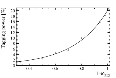
Additionally, if the particle identification is imperfect, the flavor tagging power decreases. This impact is analyzed by deliberately mislabeling hadrons with incorrect IDs. A pion is mislabelled as either a kaon or a proton with a probability of for each. This method of random mislabeling is similarly applied to kaons and protons. The tagging power varying with the correct particle identification rate is shown in Fig. 2. The tagging power is sensitive to the parameter. At the region of , where the particle identification ability is totally missing, the tagging power is degraded to around 0.
It is also worthwhile to explore how the tagging power is degraded in a realistic scenario. The momentum-dependent particle identification on CEPC was investigated in a previous study [23]. The momentum-dependent separation power is applied in this study to simulate the hadron misidentification. The seperation power quoted from [23] is used in the following way: For instance, to assign an ID to a , We generate a random variable by employing a Gaussian distribution with a mean of 0 and a standard deviation of 1. If the generated random number is less than , the ID is assigned to as . Conversely, if it is greater than , it is assigned as . Likewise, the same procedures are applied to . Additionally, the could be mistaken for either or . If the generated random number is less than , the ID of the particle is assigned as . While if the random number is larger than , the ID of is assigned to this kaon. The particles with assigned IDs are utilized to tag the initial flavor according to the tagging algorithm that was previously described. Under the intrinsic case, without considering the effects of the readout electronics, the tagging power is 19.1%. In a more realistic case, if the particle identification resolution is degraded by 30%, corresponding to a reduction of by 30% [24], the tagging power becomes 17.4%. The decrease of the tagging power with a worse PID performance is because the large difference between the abundance of and is smeared by the misidentified and .
2.5 Decay time resolution
The precision of is affected by the inaccurate determination of the decay time. The proper decay time for the meson is determined using the decay vertex position and the transverse momentum of the as follows:
| (5) |
where represents the decay vertex position in the transverse plane, denotes the transverse momentum of the meson, and represents the mass of the . The decay vertex is constructed from the four tracks from the decay. It is assumed that the primary vertex, the production point of the , is located at the origin. The resolution for determination of the primary vertex is considered negligible, given that the abundance of tracks available to reconstruct the primary vertex far exceeds those available for determining the decay location.
The decay point of the meson is determined by minimizing the value, which is calculated as the sum of the squares of the shortest distances from the vertex to each of the four helical tracks. This technique is an adaptation of the method described in Ref. [25].
To simplify the minimization process, the helical track is approximated as a straight line that is tangent to the helix at point . This point is the closest to a reference point on the helix. In this algorithm, the true decay vertex of is used as the reference point, denoted by .
Subsequently, each of the tracks is parameterized by a point and a direction . Consequently, the minimization process is replaced by the solving of a matrix equation
| (6) |
where is the decay point position and
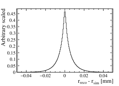
The difference between the reconstructed decay vertex position () and the truth vertex position () is shown in Fig. 3.
The transverse momentum distribution of mesons is shown in Fig. 4. The majority of these mesons have large transverse momentum because they hadronize from a high-energy -quark, which carries nearly half of the beam energy. Consequently, a substantial transverse momentum corresponds to a large Lorentz boost factor, which substantially enhances the resolution of the proper decay time.
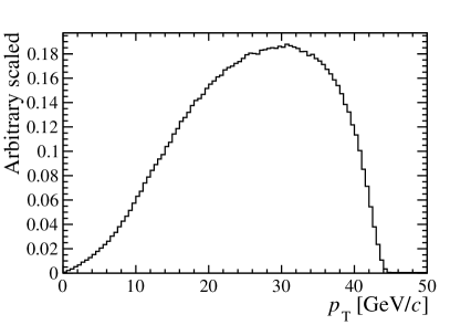
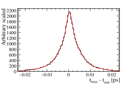
Figure 5 shows the distribution of the differences between and for the same event. Both and represent the proper decay time as calculated from Eq. (5). To derive , detector effects are not considered, and the vertex and are obtained directly from the Monte Carlo truth record. In contrast, is determined after the particles undergo detector simulation, as well as track and vertex reconstruction, using the reconstructed vertex position and transverse momentum to calculate the proper decay time. The distribution is fitted using the sum of three Gaussian functions with the same mean value. The effective time resolution is combined as
where and are the fraction and width of the i-th Gaussian function. The effective resolution of the decay time, achieved through the combined effect of the three Gaussian resolution models, is .
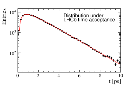
2.6 Decay time acceptance
The possible impact of non-uniform decay time-dependent efficiency, known as decay time acceptance, on the precision of measurement has been evaluated. While it was considered that different time acceptance profiles at hadron and lepton colliders might markedly influence the precision of and measurements, our findings indicate that the effect is not substantial.
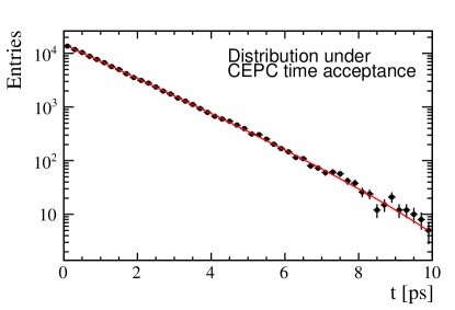
Figure 6 shows the reconstruction efficiency of the meson as a function of its proper decay time at the CEPC. The efficiency decreases at larger decay times due to the tracks of the with larger flight distances deviating increasingly from the interaction point, which complicates the reconstruction process.
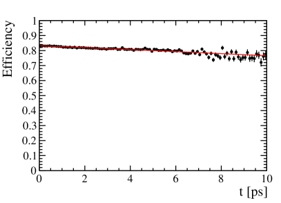
The efficiency is parameterized with a 2nd-order polynomial function . The time acceptance profile from LHCb, as referenced in Ref. [26] is , where
and
A toy Monte Carlo simulation is employed to explore the impact of the time acceptance, as elaborated in the Appendix. It is found that, with the two distinct time acceptance profiles, the fitted parameters differ by only , which will be neglected in the final results.
3 Results
3.1 Precision of , and
The above simulations show that in future -factories, the proper decay time resolution can reach , the detector
acceptanceefficiency can be as good as , and the flavor tagging power can be under a conservative assumption on the PID performance.
In addition, the acceptance and efficiency is almost flat in decay time.
Assuming the future -factory operating in Tera- mode (i.e., ), the scaling factor is . The expected resolution is .
The and depend weakly on tagging power and decay time resolution. The 3.7 times better flavor tagging power and 1.92 times better time resolution factor of CEPC, in contrast to , have negligible effects on these observables. The estimated resolution is for and for . The measured resolution of [12] is taken as the resolution of .
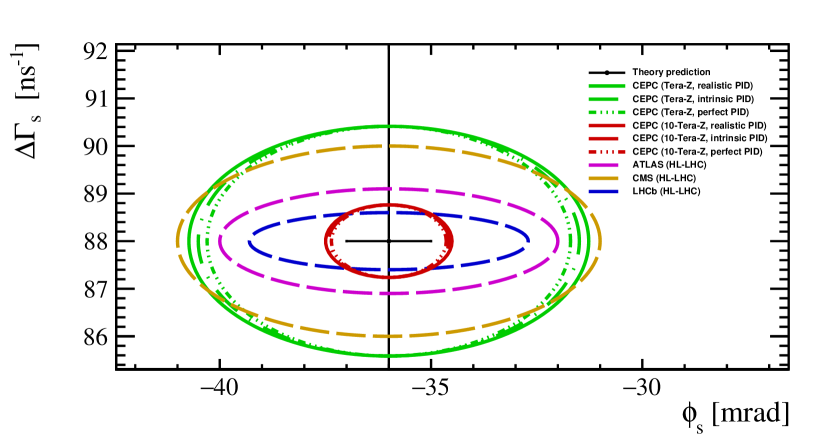
Figure 7 shows the expected confidential range ( confidential level) of . The black dot is the prediction of the standard model from CKMFitter group [1] and HQE theory calculation [4]. The green curves and red curves represent the expected precision of Tera- CEPC and 10-Tera- CEPC, respectively. The different line styles represent different PID performance assumptions, where the solid line represents the conservative PID performance assumption, which is a degradation of % of the intrinsic PID performance. The blue dashed curve represents the LHCb at the HL-LHC, projected in this study. The magenta and yellow curves are the projections from ATLAS and CMS at the HL-LHC [27, 28], respectively.
The resolution at the 10-Tera- CEPC can reach the current precision of SM prediction. All the future experiment measurements of can provide stringent constraints on the HEQ theory. The CEPC could do a better job on the measurement of the than the measurement of the because the flavor tagging and decay time resolution are excellent.
3.2 Penguin pollution
If the penguin diagram is considered in the decay, the relation between and should be corrected as
| (7) |
The shift could be expressed as
| (8) |
where and are penguin parameters, is defined through a Wolfenstein parameter , and is the angle of the Unitarity Triangle.
Control channels, such as and , were employed to determine the penguin parameters and , proposed by Ref. [29]. In this study, the LHCb measurements involving are utilized to estimate the expected precision of [30, 31]. This is based on the assumption that the findings from the measurements can be directly applied to the analysis, despite the topological differences between the two decay channels.
The observables in measurements are
| (9) |
and
| (10) |
where is the asymmetry and is an observable constructed containing the branching fraction information, assuming the symmetry.
The parameters and are polarization-dependent. The transverse components are measured at LHCb as
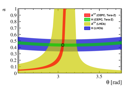
The constraints on the penguin parameters and , as defined by Eq. 9 and Eq. 10, and within the ranges of and , are shown in Fig. 8 as blue and yellow bands, respectively. At future Tera- -factory, the is expected to improve according to the Eq. (4), while the improves according to the Eq. (2). Therefore, the and are expected to be measured at CEPC with the precision
taking into account the expected improvement of LHCb Run 2 compared with LHCb Run 1. The anticipated constraints on the penguin parameters and at CEPC are represented by green and red bands in Fig. 8, with the central values of and from LHCb measurements. The expected uncertainty of and is obtained by a fit to Eq. (9) and (10), resulting in
The black contour in Fig. 8 outlines the region that falls within one standard deviation of the fitted value.
With an error propagation neglecting the correlation between and , the precision of the penguin shift is estimated as .
However, the symmetry does not always hold, and thus controlling requires additional theoretical efforts. The degradation of alongside the degradation of is shown in Fig. 9. To obtain , the expected resolution of at CEPC is used. The procedure for determining with different follows the same methodology as the aforementioned statements. The rightmost point on the Fig. 9 corresponds to , which reflects the theoretical uncertainty from the calculations in Ref. [32]. It is demonstrated that is roughly linearly dependent on , and clearly, without improved theoretical input, the control of penguin contamination will be far from satisfactory.
4 Summary
| LHCb (HL-LHC) | CEPC (Tera-Z) | CEPC/LHCb | |||
| statics | 1/284 | ||||
| Acceptanceefficiency | 10.7 | ||||
| Br | 2 | ||||
| Flavour tagging∗ | 3.7 | ||||
| Time resolution∗ () | 1.92 | ||||
| 45 | 4.7 | ||||
| scaling factor | 0.0015 | 0.0021 | 1.4 | ||
It is found that operating at Tera- mode, the expected precision can reach: , and . As shown in Table 1, the statistical disadvantage of the Tera- factory can be compensated with a much cleaner environment, good particle identification, and accurate track and vertex measurement. Without flavor tagging and time resolution benefits, the and resolution are much worse than expected for the LHC at high luminosity. Only with the 10-Tera- factory can the expected resolution of and be competitive. With the , considering only the transverse component, the penguin shift is expected to be measured as a precision of . Controlling the penguin pollution is feasible, provided that the theoretical uncertainty is managed effectively.
The study presents clear performance requirements for detector design. The flavor tagging algorithm currently relies only on the leading particle information, suggesting there is potential to refine the algorithm further to improve the precision of measurements. A tagging power of is forseenable according to the experiences from the Ref. [33]. Particle identification is critical; the performance of tagging degenerates fastly when particle misidentification occurs. Distinguishing between different hadrons using particle identification data enables more precise event selection. Moreover, robust vertex reconstruction is essential to suppress combinatorial background. While the present decay time resolution is satisfactory, further improvements in time resolution are unlikely to increase the precision of measurements.
Appendix
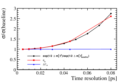
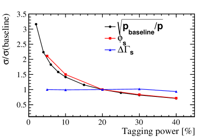
The dependent of , and on the time resolution and tagging power is investigated with toy Monte Carlo simulation. Figure 10 shows the varying resolution for and as a function of the tagging power and decay time resolution. The ratio to the baseline resolution is plotted. The baseline resolution is with the parameters and . The red line with a square marker and the blue line with a triangle marker represents the resolution from the toy Monte Carlo simulation, respectively. The black line with a circle marker represents the resolution from the analytical formula. The resolution ratio of is almost the same as that of .
The simulation provides a validation of the formula
and
and it also provides a validation that the precision of and are insensitive to the time resolution and tagging power.
The influence of decay time acceptance on the precision of is examined. Two samples, each consisting of events, are generated with the distributions and , respectively. The parameter is set as . These events are then fitted to the models and with as a free parameter, as shown in Fig. 11.
The study yielded a using the CEPC time acceptance profile, and for the LHCb time acceptance profile.
Acknowledgements
We would like to thank Jibo He, Wenbin Qian, Yuehong Xie, and Liming Zhang for their help in the discussion, polishing the manuscript, and cross-checking the results.
References
- [1] Charles, J. et al. Current status of the Standard Model CKM fit and constraints on New Physics. Phys. Rev. D 91, 073007 (2015).
- [2] Bona, M. et al. The Unitarity Triangle Fit in the Standard Model and Hadronic Parameters from Lattice QCD: A Reappraisal after the Measurements of and . JHEP 10, 081 (2006).
- [3] Workman, R. L. & Others. Review of Particle Physics. PTEP 2022, 083C01 (2022).
- [4] Neubert, M. B decays and the heavy quark expansion. Adv. Ser. Direct. High Energy Phys. 15, 239–293 (1998).
- [5] Aad, G. et al. Measurement of the -violating phase in decays in ATLAS at 13 TeV. Eur. Phys. J. C 81, 342 (2021).
- [6] Aad, G. et al. Flavor tagged time-dependent angular analysis of the decay and extraction of and the weak phase in ATLAS. Phys. Rev. D 90, 052007 (2014).
- [7] Aaltonen, T. et al. Measurement of the Bottom-Strange Meson Mixing Phase in the Full CDF Data Set. Phys. Rev. Lett. 109, 171802 (2012).
- [8] Khachatryan, V. et al. Measurement of the CP-violating weak phase and the decay width difference using the B(1020) decay channel in pp collisions at 8 TeV. Phys. Lett. B 757, 97–120 (2016).
- [9] Sirunyan, A. M. et al. Measurement of the -violating phase in the B J(1020) K+K- channel in proton-proton collisions at 13 TeV. Phys. Lett. B 816, 136188 (2021).
- [10] Abazov, V. M. et al. Measurement of the CP-violating phase using the flavor-tagged decay in 8 fb-1 of collisions. Phys. Rev. D 85, 032006 (2012).
- [11] Aaij, R. et al. Resonances and violation in and decays in the mass region above the . JHEP 08, 037 (2017).
- [12] Aaij, R. et al. Updated measurement of time-dependent CP-violating observables in decays. Eur. Phys. J. C 79, 706 (2019). [Erratum: Eur. Phys. J. C 80, 601 (2020)].
- [13] Aaij, R. et al. Measurement of the -violating phase in decays. Phys. Rev. Lett. 113, 211801 (2014).
- [14] Aaij, R. et al. First study of the CP-violating phase and decay-width difference in decays. Phys. Lett. B 762, 253–262 (2016).
- [15] Aaij, R. et al. Measurement of the -violating phase from decays in 13 TeV collisions. Phys. Lett. B 797, 134789 (2019).
- [16] Aaij, R. et al. Improved Measurement of CP Violation Parameters in Decays in the Vicinity of the (1020) Resonance. Phys. Rev. Lett. 132, 051802 (2024).
- [17] Aaij, R. et al. Physics case for an LHCb Upgrade II - Opportunities in flavour physics, and beyond, in the HL-LHC era (2018).
- [18] Dong, M. et al. CEPC Conceptual Design Report: Volume 2 - Physics & Detector (2018).
- [19] Kilian, W., Ohl, T. & Reuter, J. WHIZARD: Simulating Multi-Particle Processes at LHC and ILC. Eur. Phys. J. C 71, 1742 (2011).
- [20] Bierlich, C. et al. A comprehensive guide to the physics and usage of PYTHIA 8.3. SciPost Phys. Codeb. 2022, 8 (2022).
- [21] Agostinelli, S. et al. GEANT4–a simulation toolkit. Nucl. Instrum. Meth. A 506, 250–303 (2003).
- [22] Zyla, P. A. et al. Review of Particle Physics. PTEP 2020, 083C01 (2020).
- [23] Zhu, Y., Chen, S., Cui, H. & Ruan, M. Requirement analysis for dE/dx measurement and PID performance at the CEPC baseline detector. Nucl. Instrum. Meth. A 1047, 167835 (2023).
- [24] An, F. et al. Monte Carlo study of particle identification at the CEPC using TPC dE / dx information. Eur. Phys. J. C 78, 464 (2018).
- [25] Frühwirth, R. & Strandlie, A. Pattern Recognition, Tracking and Vertex Reconstruction in Particle Detectors Particle Acceleration and Detection (Springer, 2020).
- [26] Liu, X. Search for pentaquark state and measurement of CP violation with the LHCb detector (2019). URL https://cds.cern.ch/record/2786808. Presented 12 Dec 2019.
- [27] CP-violation measurement prospects in the channel with the upgraded ATLAS detector at the HL-LHC (2018).
- [28] CP-violation studies at the HL-LHC with CMS using decays to (2018).
- [29] Frings, P., Nierste, U. & Wiebusch, M. Penguin contributions to CP phases in decays to charmonium. Phys. Rev. Lett. 115, 061802 (2015).
- [30] Aaij, R. et al. Measurement of the CP-violating phase in decays and limits on penguin effects. Phys. Lett. B 742, 38–49 (2015).
- [31] Aaij, R. et al. Measurement of CP violation parameters and polarisation fractions in decays. JHEP 11, 082 (2015).
- [32] De Bruyn, K. Searching for penguin footprints: Towards high precision CP violation measurements in the B meson systems (2015). URL https://cds.cern.ch/record/2048174. Presented 08 Oct 2015.
- [33] Kakuno, H. et al. Neutral B flavor tagging for the measurement of mixing induced CP violation at Belle. Nucl. Instrum. Meth. A 533, 516–531 (2004).