Pros and Cons of GAN Evaluation Measures:
New Developments

Evaluation of generative models is an active area of research. Several quantitative and qualitative measures have been proposed so far. In this section, I review some of the influential measures that have inspired the researchers.

A classic approach is to compare the log-likelihoods of models. This approach, however, has several shortcomings. A model can achieve high likelihood, but low image quality, and conversely, low likelihood and high image quality. Also, kernel density estimation in high-dimensional spaces is very challenging (Theis et al., 2015).

The two most common GAN evaluation measures are Inception Score (IS) and Fréchet Inception Distance (FID). They rely on a pre-existing classifier (InceptionNet) trained on ImageNet. IS (Salimans et al., 2016) computes the KL divergence between the conditional class distribution and the marginal class distribution over the generated data. FID (Heusel et al., 2017) calculates the Wasserstein-2 (a.k.a Fréchet) distance between multivariate Gaussians fitted to the embedding space of the Inception-v3 network of generated and real images³³3To learn how to implement FID, please refer to here..

IS does not capture intra-class diversity, is insensitive to the prior distribution over labels (hence is biased towards ImageNet dataset and Inception model⁴⁴4See also here.), and is very sensitive to model parameters and implementations (Barratt and Sharma, 2018; Odena, 2019). It requires a large sample size to be reliable. A simple class-conditional model that memorizes one example per ImageNet class achieves a high IS. Using a 1D example, Barratt and Sharma (2018) show that the true underlying data distribution may achieve a lower IS than other distributions.

FID has been widely adopted because of its consistency with human inspection and sensitivity to small changes in the real distribution (e.g. slight blurring or small artifacts in synthesized images). FID, unlike IS, can detect intra-class mode collapse⁵⁵5Mode collapse happens when a generator produces data from only a few modes of the target distribution, thus failing to generate diverse enough outputs. Please see here.. The Gaussian assumption in FID calculation, however, might not hold in practice. A major drawback with FID is its high bias. The sample size to calculate FID has to be large enough (usually above 50K). Smaller sample sizes can lead to over-estimation of the actual FID (Chong and Forsyth, 2020).

While single-value metrics like IS and FID successfully capture many aspects of the generator, they lump quality and diversity evaluation and are therefore not ideal for diagnostic purposes (Precision-Recall addresses this shortcoming). Further, they continue to have a blind spot for image quality (Karras et al., 2019).

Another popular approach to evaluate GANs is manual inspection (e.g.  Denton et al. (2015); Zhou et al. (2019)). While this approach can directly tell us about the image quality, it is limited in assessing sample diversity. It is also subjective as the reviewers may incorporate their own biases and opinions. It also requires knowledge of what is realistic and what is not for the target domain which might be hard to learn in some domains (e.g. medical domain⁶⁶6For example, to tell whether a GAN can generate X-rays with pneumonia in them, it is better to ask doctors rather than Amazon Mechanical Turk workers!). Further, it is constrained by the number of images that can be reviewed in a reasonable time prohibiting its usage during model development. Finally, due to the subtle differences in experimental protocols (e.g. user interface design, fees, duration), it is often difficult to replicate the results across different publications.

This paper is organized as follows. Recently proposed evaluation measures are categorized under quantitative and qualitative measures and are covered in sections 2 and 3, respectively⁷⁷7Some methods may fall in both categories.. In section 4, I then discuss some benchmark and model comparison studies as well as analysis works. Finally, section 5 highlights some major points and offers suggestions for future research in GAN evaluation. Note that some of the works reviewed here have not been accepted in prior published work and may have not been peer reviewed. Therefore, they should be treated with additional caution in the absence of widespread usage.

FID scores computed with classification-pretrained embeddings have been shown to correlate well with human evaluations (Heusel et al., 2017). Meanwhile, they can be misleading as they are biased towards ImageNet. On non-ImageNet datasets, FID can result in inadequate evaluation. Morozov et al. (2020) advocate for using self-supervised representations to evaluate GANs on the established non-ImageNet benchmarks¹¹¹¹11https://github.com/stanis-morozov/self-supervised-gan-eval. They show that representations, typically obtained via contrastive or clustering-based approaches, provide better transfer to new tasks and domains, and thus can serve as more universal embeddings of natural images. Further, they demonstrate that self-supervised representations produce a more reasonable ranking of models and often improve the sample efficiency of FID.

These methods measure disentanglement in the representations learned by generative models, and are useful for improving the generalization, robustness, and interpretability of models.

Ravuri and Vinyals (2019) propose a measure that is in essence similar to the “Classification Performance” discussed in Borji (2019). They argue that if a generative model is learning the data distribution in a perceptually meaningful space then it should perform well in downstream tasks. They use class-conditional generative models from a number of generative models such as GANs and VAEs to infer the class labels of real data. They then train an image classifier using only synthetic data and use it to predict labels of real images in the test set. Their findings are as follows: a) when using a state-of-the-art GAN (BigGAN-deep by Brock et al. (2018)), Top-1 and Top-5 accuracies decrease by 27.9% and 41.6%, respectively, compared to the original data, b) CAS automatically identifies particular classes for which generative models fail to capture the data distribution (Fig. 6), and c) IS and FID are neither predictive of CAS, nor useful when evaluating non-GAN models.

Meehan et al. (2020) formalize a notion of overfitting called data-copying where a generative model memorizes the training samples or their small variations (Fig. 7). They provide a three sample test for detecting data-copying that uses the training set, a separate held-out sample from the target distribution, and a generated sample from the model. The key insight is that an overfitted GAN generates samples that are on average closer to the training samples, therefore the average distance of generated samples to training samples is smaller than the corresponding distances between held-out test samples and the training samples. They also divide the instance space into cells and conduct their test separately in each cell. This is because, as they argue, generative models tend to behave differently in different regions of space.

Zhao et al. (2018)¹⁶¹⁶16Please see also the subsection on “Evaluating Mode Drop and Mode Collapse” in Borji (2019). utilize carefully designed training datasets to characterize how existing models generate novel attributes and their combinations. Some of their findings are as follows. When presented with a training set with all images having exactly 3 objects, both GANs and VAEs typically generate 2-5 objects (Fig. 8.B). Over a multi-modal training distribution (e.g. images with either 2 or 10 objects), the model acts as if it is trained separately on each mode, and it averages the two modes. When the modes are close to each other (e.g. 2 and 4 objects), the learned distribution assigns higher probability to the mean number of objects (3 in this example), even though there was no image with 3 objects in the training set (Fig. 8.C). When the training set contains certain combinations (e.g. red cubes but not yellow cubes; Fig. 8.D), the model memorizes the combinations in the training set when it contains a small number of them (e.g. 20), and generates novel combinations when there is more variety (e.g. 80). Xuan et al. (2019) made a similar observation shown in Fig. 9. On a geometric-object training dataset where the number of objects for each training image is fixed, they found a variable number of objects in generated images. Some other studies that have investigated GAN generalization include O’Brien et al. (2018); van Steenkiste et al. (2020).

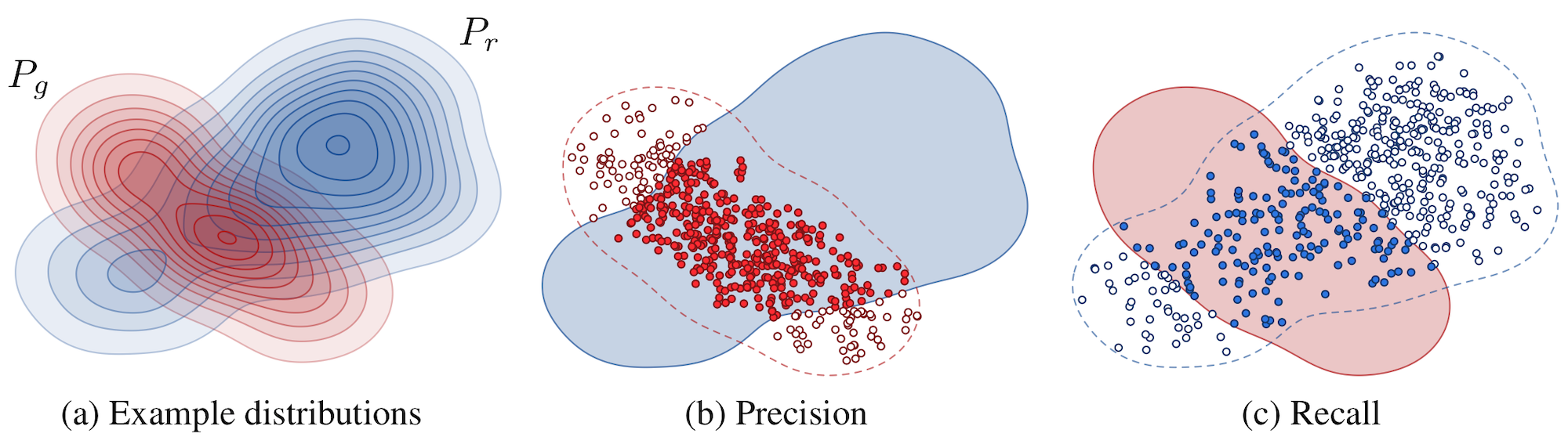
Sajjadi et al. (2018) propose to use precision and recall to explicitly quantify the trade off between quality (precision) and coverage (recall). Precision measures the similarity of generated instances to the real ones and recall measures the ability of a generator to synthesize all instances found in the training set (Fig. 10). P&R curves can distinguish mode-collapse (poor recall) and bad quality (poor precision). Some new ideas based on P&R are summarized below.

Grnarova et al. (2019) leverage the notion of duality gap from game theory to propose a domain-agnostic and computationally-efficient measure that can be used to assess different models as well as monitoring the progress of a single model throughout training. Intuitively, duality gap measures the sub-optimality (w.r.t. an equilibrium) of a given solution (G,D) where G and D and the generator and the discriminator, respectively. They also show that their measure highly correlates with FID on natural image datasets, and can also be used in other modalities such as text and sound. Further, their measure requires no labels or a pretrained classifier, making it domain agnostic. In a follow-up work, Sidheekh et al. (2021) extend the notion of duality gap to proximal duality gap that is applicable to the general context of training GANs.

A number of studies (e.g.  Durall et al. (2020); Frank et al. (2020); Dzanic et al. (2019); Zeng et al. (2017)) have shown that current generators are unable to correctly approximate the spectral distributions of real data. Durall et al. (2020) showed that up-scaling operations commonly used in GANs (e.g. up-convolutions) alter the spectral properties of the images causing high frequency distortions in the output. This can be seen in the average azimuthal integration of the power spectrum shown in the top panel of Fig. 13. Based on this observation, they proposed a novel spectral regularization term to compensate spectral distortions. They also proposed a very simple but highly accurate detector for generated images and videos, i.e. a DeepFake detector.

Almost all existing metrics are solely for evaluating models that generative image. They do not take into account the corresponding text in the context of text-to-image generation. Thus, they may be fooled by a network that ignores the textual input and only focuses on generating realistic looking images. To remedy this shortcoming, Ding et al. (2021) introduce the caption score to evaluate the correspondence between images and text. This score measures the quality and accuracy for text-image generation at a finer granularity than FID and Inception Score (IS), and is defined as:

where $t$ is a sequence of text tokens and $x$ is the image. The higher the CapS, the better. In addition to CapS, they also report results using other measures such as FID and IS.

A commonly used metric to evaluate generative models of text is the perplexity. It measures the probability for a sentence to be produced by a language model that has been trained on a dataset:

$\text{perplexity }=\prod_{t=1}^{T}\left(\frac{1}{P_{\mathrm{LM}}\left(\bm{x}^{(t+1)}\mid\bm{x}^{(t)},\ldots,\bm{x}^{(1)}\right)}\right)^{1/T}$

Zhou et al. (2019) propose a human-in-the-loop evaluation approach that is grounded in psychophysics research on visual perception (Fig. 14). They introduce two variants. The first one measures visual perception under adaptive time constraints to determine the threshold at which a model’s outputs appear real (e.g. 250 ms). The second variant is less expensive and measures human error rate on fake and real images without time constraints¹⁸¹⁸18An important point when conducting experiments of this sort (e.g.  Denton et al. (2015)) is to make sure that real and generated images are shuffled during the presentation. Otherwise, subjects maybe able to guess what type of images are shown in a session from the first few images, if all the images in the session in either real or fake.. Kolchinski et al. (2019) propose an approach to approximate HYPE and report 66% accuracy in predicting human scores of image realism, matching the human inter-rater agreement rate. A major drawback with human evaluation approaches such as HYPE is scaling them. One way to remedy this is to train a model from human judgments and interact with a person only when the model is not certain. HYPE is more reliable compared to automated ones but cannot be used for monitoring the training process.

Wang et al. (2020b) outline a method called Neuroscore using neural signals and rapid serial visual presentation (RSVP) to directly measure human perceptual response to generated stimuli. Participants are instructed to attend to target images (real and generated) amongst a larger set of non-target images (left panel in Fig. 15). This paradigm, known as the oddball paradigm, is commonly used to elicit the P300 event-related potential (ERP), which is a positive voltage deflection typically occurring between 300 ms and 600 ms after the appearance of a rare visual target. Fig. 15 shows a depiction of this approach. Wang et al. show that Neuroscore is more consistent with human judgments compared to the conventional metrics. They also trained a convolutional neural network to predict Neuroscore from GAN-generated images directly without the need for neural responses.

Bau et al. (2019) visualize mode collapse at both distribution level and instance level. They employ a semantic segmentation network to compare the distribution of segmented objects in the generated images versus the real images. Differences in statistics reveal object classes that are omitted by a GAN. Their approach allows to visualize the GAN’s omissions for an omitted class and to compare differences between individual photos and their approximate inversions by a GAN. Fig. 16 illustrates this approach.

Jahanian et al. (2019) propose a method to quantify the degree to which basic visual transformations are achieved by navigating the latent space of a GAN (See Fig. 17). They first learn a $N$-dimensional vector representing the optimal path in the latent space for a given transformation. Formally, the task it to learn the walk $w$ by minimizing the following objective function:

where $\alpha$ is the step size, and $\mathcal{L}$ is the distance between the generated image $G(z+\alpha w)$ after taking an $\alpha$-step in the latent direction and the target image edit($G(z)$, $\alpha$). The latter is the new image derived from the source image $G(z)$. To quantify how well a desired image manipulation under each transformation is achieved, the distributions of a given attribute (e.g. “luminance”) in the real data and generated images (after walking in latent space) are compared.

Bau et al. (2018) propose a technique to dissect and visualize the inner workings of an image generator¹⁹¹⁹19A demo of this work is available at here.. The main idea is to identify GAN units (i.e. generator neurons) that are responsible for semantic concepts and objects (such as tree, sky, and clouds) in the generated images. Having this level of granularity into the neurons allows editing existing images (e.g. to add or remove trees as shown in Fig. 18) by forcefully activating and deactivating (ablating) the corresponding units for the desired objects. Their technique also allows finding artifacts in the generated images and hence can be used to evaluate and improve GANs. A similar approach has been proposed in Park et al. (2019) for semantic manipulation and editing of GAN generated images²⁰²⁰20See here for an illustration..

Wang et al. (2020a) ask whether it is possible to create a “universal” detector to distinguish real images from synthetic ones using a dataset of synthetic images generated by 11 CNN-based generative models. See Fig. 19. With careful pre- and post-processing and data augmentation, they show that an image classifier trained on only one specific CNN generator is able to generalize well to unseen architectures, datasets, and training methods. They highlight that today’s CNN-generated images share common systematic flaws, preventing them from achieving realistic image generation. Similar works have been reported in Chai et al. (2020); Yu et al. (2019). In alignment with these results, Gragnaniello et al. (2021) also conclude that we are still far from having reliable tools for GAN image detection.

Following previous works (e.g.  Lucic et al. (2017); Shmelkov et al. (2018)), new studies have investigated formulating good criteria for GAN evaluation, or have conducted systematic GAN benchmarks. Gulrajani et al. (2020) argue that a good evaluation measure should not have a trivial solution (e.g. memorizing the dataset) and show that many scores such as IS and FID can be won by simply memorizing the training data (Fig. 20). They suggest that a necessary condition for a metric not to behave this way is to have a large number of samples. They also propose a measure based on neural network divergences (NND). NND works by training a discriminative model to discriminate between samples of the generative model and samples from a held-out test set. The poorer the discriminative model performs, the better the generative model is. Through experimental validation, they show that NND can effectively measure diversity, sample quality, and generalization. Lee and Town (2020) introduce Mimicry²¹²¹21https://github.com/kwotsin/mimicry, a lightweight PyTorch library that provides implementations of popular GANs and evaluation metrics to closely reproduce reported scores in the literature. They also compare several GANs on seven widely-used datasets by training them under the same conditions, and evaluating them using three popular GAN metrics. Some tutorials and interaction tools have also been developed to understand, visualize, and evaluate GANs²²²²22See this link and https://poloclub.github.io/ganlab/..

Also mention that deepfakes might be detected because they have different spectral properties than real images. See for example Durall et al. (2020)

Fairness and bias in ML algorithms, datasets, and commercial products have become growing concerns recently (e.g.  Buolamwini and Gebru (2018)) and have attracted widespread attention from public and media²³²³23https://thegradient.pub/pulse-lessons/. Even without a single precise definition for fairness (Verma and Rubin, 2018), it is still possible to observe the lack of fairness across many domains and models, with GANs being no exception. Some recent works (e.g.  Xu et al. (2018); Yu et al. (2020) have tried to mitigate the bias in GANs or use GANs to reduce bias in other ML algorithms (e.g.  Sattigeri et al. (2019); McDuff et al. (2019)). Bias can enter a model during training (through data, labeling, architecture), evaluation (such as who created the evaluation measure), as well as deployment (how is the model being distributed and for what purposes). Therefore it is critical to address these aspects when evaluating and comparing generative models.

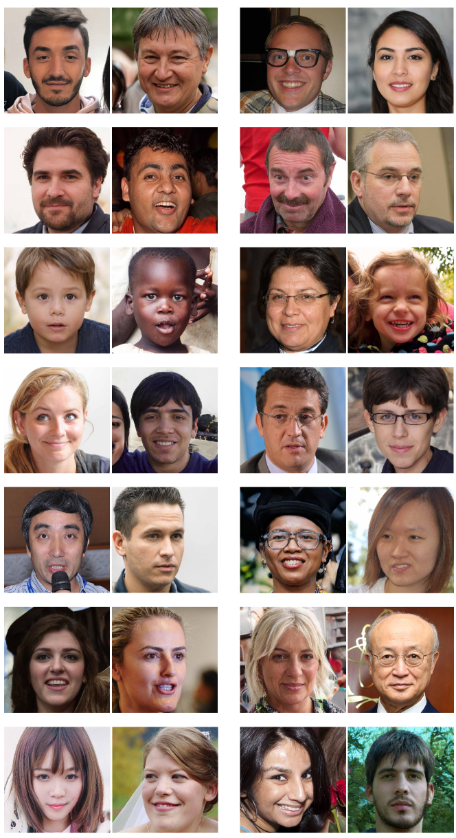
A alarming application of generative models is fabricating fake content²⁴²⁴24Some concerns can be found at these links 1, 2, 3, and 4. It is thus crucial to develop tools and techniques to detect and limit their use (See Tolosana et al. (2020) for a survey on deepfakes). There is a natural connection between deepfake detection and GAN evaluation. Obviously, as generative models improve, it becomes increasingly harder for a human to distinguish between what is real and what is fake (manipulated images, videos, text, and audio). Telling the degree of fakeness of an image or video directly tells us about the performance of a generator. Even over faces, where generative models excel, it is still possible to detect fake images (Fig. 21), although in some cases it can be very daunting (Fig. 22). Difficulty of deepfake detection for humans is also category dependent, with some categories such as faces, cats, and dogs being easier than bedrooms or cluttered scenes (Fig. 23). Fortunately, or unfortunately, it is still possible to build deep networks that can detect the subtle artifacts in the doctored images (e.g. using the universal detectors mentioned above (Wang et al., 2020a; Chai et al., 2020)). Moving forward, it is important to study whether and how GAN evaluation measures can help us mitigate the threat from deepfakes.

References

- Alaa et al. (2021) Alaa, A.M., van Breugel, B., Saveliev, E., van der Schaar, M., 2021. How faithful is your synthetic data? sample-level metrics for evaluating and auditing generative models. arXiv preprint arXiv:2102.08921 .
- Bai et al. (2021) Bai, C.Y., Lin, H.T., Raffel, C., Kan, W.C.w., 2021. On training sample memorization: Lessons from benchmarking generative modeling with a large-scale competition. arXiv preprint arXiv:2106.03062 .
- Barannikov et al. (2021) Barannikov, S., Trofimov, I., Sotnikov, G., Trimbach, E., Korotin, A., Filippov, A., Burnaev, E., 2021. Manifold topology divergence: a framework for comparing data manifolds. arXiv preprint arXiv:2106.04024 .
- Barratt and Sharma (2018) Barratt, S., Sharma, R., 2018. A note on the inception score. arXiv preprint arXiv:1801.01973 .
- Barua et al. (2019) Barua, S., Ma, X., Erfani, S.M., Houle, M.E., Bailey, J., 2019. Quality evaluation of gans using cross local intrinsic dimensionality. arXiv preprint arXiv:1905.00643 .
- Bau et al. (2018) Bau, D., Zhu, J.Y., Strobelt, H., Zhou, B., Tenenbaum, J.B., Freeman, W.T., Torralba, A., 2018. Gan dissection: Visualizing and understanding generative adversarial networks. arXiv preprint arXiv:1811.10597 .
- Bau et al. (2019) Bau, D., Zhu, J.Y., Wulff, J., Peebles, W., Strobelt, H., Zhou, B., Torralba, A., 2019. Seeing what a gan cannot generate, in: Proceedings of the IEEE International Conference on Computer Vision, pp. 4502–4511.
- Bińkowski et al. (2018) Bińkowski, M., Sutherland, D.J., Arbel, M., Gretton, A., 2018. Demystifying mmd gans. arXiv preprint arXiv:1801.01401 .
- Bond-Taylor et al. (2021) Bond-Taylor, S., Leach, A., Long, Y., Willcocks, C.G., 2021. Deep generative modelling: A comparative review of vaes, gans, normalizing flows, energy-based and autoregressive models. arXiv preprint arXiv:2103.04922 .
- Borji (2019) Borji, A., 2019. Pros and cons of gan evaluation measures. Computer Vision and Image Understanding 179, 41–65.
- Brock et al. (2018) Brock, A., Donahue, J., Simonyan, K., 2018. Large scale gan training for high fidelity natural image synthesis. arXiv preprint arXiv:1809.11096 .
- Buolamwini and Gebru (2018) Buolamwini, J., Gebru, T., 2018. Gender shades: Intersectional accuracy disparities in commercial gender classification, in: Conference on fairness, accountability and transparency, PMLR. pp. 77–91.
- van den Burg and Williams (2021) van den Burg, G.J., Williams, C.K., 2021. On memorization in probabilistic deep generative models. arXiv preprint arXiv:2106.03216 .
- Carreira and Zisserman (2017) Carreira, J., Zisserman, A., 2017. Quo vadis, action recognition? a new model and the kinetics dataset, in: proceedings of the IEEE Conference on Computer Vision and Pattern Recognition, pp. 6299–6308.
- Casanova et al. (2020) Casanova, A., Drozdzal, M., Romero-Soriano, A., 2020. Generating unseen complex scenes: are we there yet? arXiv preprint arXiv:2012.04027 .
- Chai et al. (2020) Chai, L., Bau, D., Lim, S.N., Isola, P., 2020. What makes fake images detectable? understanding properties that generalize, in: European Conference on Computer Vision, Springer. pp. 103–120.
- Chen et al. (2018) Chen, L., Li, Z., Maddox, R.K., Duan, Z., Xu, C., 2018. Lip movements generation at a glance, in: Proceedings of the European Conference on Computer Vision (ECCV), pp. 520–535.
- Chong and Forsyth (2020) Chong, M.J., Forsyth, D., 2020. Effectively unbiased fid and inception score and where to find them, in: Proceedings of the IEEE/CVF Conference on Computer Vision and Pattern Recognition, pp. 6070–6079.
- De and Masilamani (2013) De, K., Masilamani, V., 2013. Image sharpness measure for blurred images in frequency domain. Procedia Engineering 64, 149–158.
- Denton et al. (2015) Denton, E., Chintala, S., Szlam, A., Fergus, R., 2015. Deep generative image models using a laplacian pyramid of adversarial networks. arXiv preprint arXiv:1506.05751 .
- Ding et al. (2021) Ding, M., Yang, Z., Hong, W., Zheng, W., Zhou, C., Yin, D., Lin, J., Zou, X., Shao, Z., Yang, H., et al., 2021. Cogview: Mastering text-to-image generation via transformers. arXiv preprint arXiv:2105.13290 .
- Djolonga et al. (2020) Djolonga, J., Lucic, M., Cuturi, M., Bachem, O., Bousquet, O., Gelly, S., 2020. Precision-recall curves using information divergence frontiers, in: International Conference on Artificial Intelligence and Statistics, pp. 2550–2559.
- Durall et al. (2020) Durall, R., Keuper, M., Keuper, J., 2020. Watch your up-convolution: Cnn based generative deep neural networks are failing to reproduce spectral distributions, in: Proceedings of the IEEE/CVF Conference on Computer Vision and Pattern Recognition, pp. 7890–7899.
- Dzanic et al. (2019) Dzanic, T., Shah, K., Witherden, F., 2019. Fourier spectrum discrepancies in deep network generated images. arXiv preprint arXiv:1911.06465 .
- Frank et al. (2020) Frank, J., Eisenhofer, T., Schönherr, L., Fischer, A., Kolossa, D., Holz, T., 2020. Leveraging frequency analysis for deep fake image recognition, in: International Conference on Machine Learning, PMLR. pp. 3247–3258.
- Goodfellow et al. (2014) Goodfellow, I.J., Pouget-Abadie, J., Mirza, M., Xu, B., Warde-Farley, D., Ozair, S., Courville, A., Bengio, Y., 2014. Generative adversarial networks. arXiv preprint arXiv:1406.2661 .
- Gragnaniello et al. (2021) Gragnaniello, D., Cozzolino, D., Marra, F., Poggi, G., Verdoliva, L., 2021. Are gan generated images easy to detect? a critical analysis of the state-of-the-art. arXiv preprint arXiv:2104.02617 .
- Grnarova et al. (2019) Grnarova, P., Levy, K.Y., Lucchi, A., Perraudin, N., Goodfellow, I., Hofmann, T., Krause, A., 2019. A domain agnostic measure for monitoring and evaluating gans, in: Advances in Neural Information Processing Systems, pp. 12092–12102.
- Gulrajani et al. (2020) Gulrajani, I., Raffel, C., Metz, L., 2020. Towards gan benchmarks which require generalization. arXiv preprint arXiv:2001.03653 .
- Heusel et al. (2017) Heusel, M., Ramsauer, H., Unterthiner, T., Nessler, B., Hochreiter, S., 2017. Gans trained by a two time-scale update rule converge to a local nash equilibrium. arXiv preprint arXiv:1706.08500 .
- Hudson and Zitnick (2021) Hudson, D.A., Zitnick, C.L., 2021. Generative adversarial transformers. arXiv preprint arXiv:2103.01209 .
- Iqbal and Qureshi (2020) Iqbal, T., Qureshi, S., 2020. The survey: Text generation models in deep learning. Journal of King Saud University-Computer and Information Sciences .
- Jahanian et al. (2019) Jahanian, A., Chai, L., Isola, P., 2019. On the”steerability" of generative adversarial networks. arXiv preprint arXiv:1907.07171 .
- Jiang et al. (2021) Jiang, Y., Chang, S., Wang, Z., 2021. Transgan: Two transformers can make one strong gan. arXiv preprint arXiv:2102.07074 .
- Karras et al. (2019) Karras, T., Laine, S., Aila, T., 2019. A style-based generator architecture for generative adversarial networks, in: Proceedings of the IEEE conference on computer vision and pattern recognition, pp. 4401–4410.
- Karras et al. (2020) Karras, T., Laine, S., Aittala, M., Hellsten, J., Lehtinen, J., Aila, T., 2020. Analyzing and improving the image quality of stylegan, in: Proceedings of the IEEE/CVF Conference on Computer Vision and Pattern Recognition, pp. 8110–8119.
- Khrulkov and Oseledets (2018) Khrulkov, V., Oseledets, I., 2018. Geometry score: A method for comparing generative adversarial networks, in: International Conference on Machine Learning, PMLR. pp. 2621–2629.
- Kingma and Welling (2013) Kingma, D.P., Welling, M., 2013. Auto-encoding variational bayes. arXiv preprint arXiv:1312.6114 .
- Kolchinski et al. (2019) Kolchinski, Y.A., Zhou, S., Zhao, S., Gordon, M., Ermon, S., 2019. Approximating human judgment of generated image quality. arXiv preprint arXiv:1912.12121 .
- Kynkäänniemi et al. (2019) Kynkäänniemi, T., Karras, T., Laine, S., Lehtinen, J., Aila, T., 2019. Improved precision and recall metric for assessing generative models. arXiv preprint arXiv:1904.06991 .
- Lee and Town (2020) Lee, K.S., Town, C., 2020. Mimicry: Towards the reproducibility of gan research. arXiv preprint arXiv:2005.02494 .
- Liu et al. (2021) Liu, M.Y., Huang, X., Yu, J., Wang, T.C., Mallya, A., 2021. Generative adversarial networks for image and video synthesis: Algorithms and applications. Proceedings of the IEEE .
- Liu et al. (2018) Liu, S., Wei, Y., Lu, J., Zhou, J., 2018. An improved evaluation framework for generative adversarial networks. arXiv preprint arXiv:1803.07474 .
- Liu et al. (2015) Liu, Z., Luo, P., Wang, X., Tang, X., 2015. Deep learning face attributes in the wild, in: Proceedings of the IEEE international conference on computer vision, pp. 3730–3738.
- Lucic et al. (2017) Lucic, M., Kurach, K., Michalski, M., Gelly, S., Bousquet, O., 2017. Are gans created equal? a large-scale study. arXiv preprint arXiv:1711.10337 .
- Mathiasen and Hvilshøj (2020) Mathiasen, A., Hvilshøj, F., 2020. Fast fr’echet inception distance. arXiv preprint arXiv:2009.14075 .
- McDuff et al. (2019) McDuff, D., Ma, S., Song, Y., Kapoor, A., 2019. Characterizing bias in classifiers using generative models. arXiv preprint arXiv:1906.11891 .
- Meehan et al. (2020) Meehan, C., Chaudhuri, K., Dasgupta, S., 2020. A non-parametric test to detect data-copying in generative models. arXiv preprint arXiv:2004.05675 .
- Morozov et al. (2020) Morozov, S., Voynov, A., Babenko, A., 2020. On self-supervised image representations for gan evaluation, in: International Conference on Learning Representations.
- Naeem et al. (2020) Naeem, M.F., Oh, S.J., Uh, Y., Choi, Y., Yoo, J., 2020. Reliable fidelity and diversity metrics for generative models. arXiv preprint arXiv:2002.09797 .
- Narvekar and Karam (2009) Narvekar, N.D., Karam, L.J., 2009. A no-reference perceptual image sharpness metric based on a cumulative probability of blur detection, in: 2009 International Workshop on Quality of Multimedia Experience, IEEE. pp. 87–91.
- Nash et al. (2021) Nash, C., Menick, J., Dieleman, S., Battaglia, P.W., 2021. Generating images with sparse representations. arXiv preprint arXiv:2103.03841 .
- O’Brien et al. (2018) O’Brien, S., Groh, M., Dubey, A., 2018. Evaluating generative adversarial networks on explicitly parameterized distributions. arXiv preprint arXiv:1812.10782 .
- Odena (2019) Odena, A., 2019. Open questions about generative adversarial networks. Distill 4, e18.
- Oord et al. (2016) Oord, A.v.d., Kalchbrenner, N., Vinyals, O., Espeholt, L., Graves, A., Kavukcuoglu, K., 2016. Conditional image generation with pixelcnn decoders. arXiv preprint arXiv:1606.05328 .
- Oprea et al. (2020) Oprea, S., Martinez-Gonzalez, P., Garcia-Garcia, A., Castro-Vargas, J.A., Orts-Escolano, S., Garcia-Rodriguez, J., Argyros, A., 2020. A review on deep learning techniques for video prediction. IEEE Transactions on Pattern Analysis and Machine Intelligence .
- Park et al. (2019) Park, T., Liu, M.Y., Wang, T.C., Zhu, J.Y., 2019. Semantic image synthesis with spatially-adaptive normalization, in: Proceedings of the IEEE/CVF Conference on Computer Vision and Pattern Recognition, pp. 2337–2346.
- Parmar et al. (2021) Parmar, G., Zhang, R., Zhu, J.Y., 2021. On buggy resizing libraries and surprising subtleties in fid calculation. arXiv preprint arXiv:2104.11222 .
- Preuer et al. (2018) Preuer, K., Renz, P., Unterthiner, T., Hochreiter, S., Klambauer, G., 2018. Fréchet chemnet distance: a metric for generative models for molecules in drug discovery. Journal of chemical information and modeling 58, 1736–1741.
- Ramesh et al. (2021) Ramesh, A., Pavlov, M., Goh, G., Gray, S., Voss, C., Radford, A., Chen, M., Sutskever, I., 2021. Zero-shot text-to-image generation. arXiv preprint arXiv:2102.12092 .
- Ravuri and Vinyals (2019) Ravuri, S., Vinyals, O., 2019. Classification accuracy score for conditional generative models, in: Advances in Neural Information Processing Systems, pp. 12268–12279.
- Razavi et al. (2019) Razavi, A., Oord, A.v.d., Vinyals, O., 2019. Generating diverse high-fidelity images with vq-vae-2. arXiv preprint arXiv:1906.00446 .
- Roblek et al. (2019) Roblek, D., Kilgour, K., Sharifi, M., Zuluaga, M., 2019. Fr’echet audio distance: A reference-free metric for evaluating music enhancement algorithms .
- Sajjadi et al. (2018) Sajjadi, M.S., Bachem, O., Lucic, M., Bousquet, O., Gelly, S., 2018. Assessing generative models via precision and recall, in: Advances in Neural Information Processing Systems, pp. 5228–5237.
- Salimans et al. (2016) Salimans, T., Goodfellow, I., Zaremba, W., Cheung, V., Radford, A., Chen, X., 2016. Improved techniques for training gans. arXiv preprint arXiv:1606.03498 .
- Sattigeri et al. (2019) Sattigeri, P., Hoffman, S.C., Chenthamarakshan, V., Varshney, K.R., 2019. Fairness gan: Generating datasets with fairness properties using a generative adversarial network. IBM Journal of Research and Development 63, 3–1.
- Shmelkov et al. (2018) Shmelkov, K., Schmid, C., Alahari, K., 2018. How good is my gan?, in: Proceedings of the European Conference on Computer Vision (ECCV), pp. 213–229.
- Shoemake (1985) Shoemake, K., 1985. Animating rotation with quaternion curves, in: Proceedings of the 12th annual conference on Computer graphics and interactive techniques, pp. 245–254.
- Sidheekh et al. (2021) Sidheekh, S., Aimen, A., Krishnan, N.C., 2021. Characterizing gan convergence through proximal duality gap. arXiv preprint arXiv:2105.04801 .
- Simon et al. (2019) Simon, L., Webster, R., Rabin, J., 2019. Revisiting precision and recall definition for generative model evaluation. arXiv preprint arXiv:1905.05441 .
- Simonyan and Zisserman (2014) Simonyan, K., Zisserman, A., 2014. Very deep convolutional networks for large-scale image recognition. arXiv preprint arXiv:1409.1556 .
- Soloveitchik et al. (2021) Soloveitchik, M., Diskin, T., Morin, E., Wiesel, A., 2021. Conditional frechet inception distance. arXiv preprint arXiv:2103.11521 .
- van Steenkiste et al. (2020) van Steenkiste, S., Kurach, K., Schmidhuber, J., Gelly, S., 2020. Investigating object compositionality in generative adversarial networks. Neural Networks 130, 309–325.
- Tevet et al. (2018) Tevet, G., Habib, G., Shwartz, V., Berant, J., 2018. Evaluating text gans as language models. arXiv preprint arXiv:1810.12686 .
- Theis et al. (2015) Theis, L., Oord, A.v.d., Bethge, M., 2015. A note on the evaluation of generative models. arXiv preprint arXiv:1511.01844 .
- Tolosana et al. (2020) Tolosana, R., Vera-Rodriguez, R., Fierrez, J., Morales, A., Ortega-Garcia, J., 2020. Deepfakes and beyond: A survey of face manipulation and fake detection. Information Fusion 64, 131–148.
- Tsitsulin et al. (2019) Tsitsulin, A., Munkhoeva, M., Mottin, D., Karras, P., Bronstein, A., Oseledets, I., Müller, E., 2019. The shape of data: Intrinsic distance for data distributions. arXiv preprint arXiv:1905.11141 .
- Tulyakov et al. (2018) Tulyakov, S., Liu, M.Y., Yang, X., Kautz, J., 2018. Mocogan: Decomposing motion and content for video generation, in: Proceedings of the IEEE conference on computer vision and pattern recognition, pp. 1526–1535.
- Unterthiner et al. (2019) Unterthiner, T., van Steenkiste, S., Kurach, K., Marinier, R., Michalski, M., Gelly, S., 2019. Fvd: A new metric for video generation .
- Verma and Rubin (2018) Verma, S., Rubin, J., 2018. Fairness definitions explained, in: 2018 ieee/acm international workshop on software fairness (fairware), IEEE. pp. 1–7.
- Wang et al. (2020a) Wang, S.Y., Wang, O., Zhang, R., Owens, A., Efros, A.A., 2020a. Cnn-generated images are surprisingly easy to spot… for now, in: Proceedings of the IEEE Conference on Computer Vision and Pattern Recognition.
- Wang et al. (2020b) Wang, Z., Healy, G., Smeaton, A.F., Ward, T.E., 2020b. Use of neural signals to evaluate the quality of generative adversarial network performance in facial image generation. Cognitive Computation 12, 13–24.
- Wang et al. (2019) Wang, Z., She, Q., Ward, T.E., 2019. Generative adversarial networks in computer vision: A survey and taxonomy. arXiv preprint arXiv:1906.01529 .
- Xu et al. (2018) Xu, D., Yuan, S., Zhang, L., Wu, X., 2018. Fairgan: Fairness-aware generative adversarial networks, in: 2018 IEEE International Conference on Big Data (Big Data), IEEE. pp. 570–575.
- Xuan et al. (2019) Xuan, J., Yang, Y., Yang, Z., He, D., Wang, L., 2019. On the anomalous generalization of gans. arXiv preprint arXiv:1909.12638 .
- Yang et al. (2018) Yang, C., Wang, Z., Zhu, X., Huang, C., Shi, J., Lin, D., 2018. Pose guided human video generation, in: Proceedings of the European Conference on Computer Vision (ECCV), pp. 201–216.
- Yu et al. (2015) Yu, F., Seff, A., Zhang, Y., Song, S., Funkhouser, T., Xiao, J., 2015. Lsun: Construction of a large-scale image dataset using deep learning with humans in the loop. arXiv preprint arXiv:1506.03365 .
- Yu et al. (2019) Yu, N., Davis, L.S., Fritz, M., 2019. Attributing fake images to gans: Learning and analyzing gan fingerprints, in: Proceedings of the IEEE/CVF International Conference on Computer Vision, pp. 7556–7566.
- Yu et al. (2020) Yu, N., Li, K., Zhou, P., Malik, J., Davis, L., Fritz, M., 2020. Inclusive gan: Improving data and minority coverage in generative models, in: European Conference on Computer Vision, Springer. pp. 377–393.
- Zeng et al. (2017) Zeng, Y., Lu, H., Borji, A., 2017. Statistics of deep generated images. arXiv preprint arXiv:1708.02688 .
- Zhang et al. (2018) Zhang, R., Isola, P., Efros, A.A., Shechtman, E., Wang, O., 2018. The unreasonable effectiveness of deep features as a perceptual metric, in: Proceedings of the IEEE conference on computer vision and pattern recognition, pp. 586–595.
- Zhao et al. (2018) Zhao, S., Ren, H., Yuan, A., Song, J., Goodman, N., Ermon, S., 2018. Bias and generalization in deep generative models: An empirical study, in: Advances in Neural Information Processing Systems, pp. 10792–10801.
- Zhou et al. (2019) Zhou, S., Gordon, M., Krishna, R., Narcomey, A., Fei-Fei, L.F., Bernstein, M., 2019. Hype: A benchmark for human eye perceptual evaluation of generative models, in: Advances in Neural Information Processing Systems, pp. 3449–3461.