Proofs and additional experiments on Second order techniques for learning time-series with structural breaks

Takayuki Osogami
IBM Research - Tokyo
[email protected]

Abstract

We provide complete proofs of the lemmas about the properties of the regularized loss function that is used in the second order techniques for learning time-series with structural breaks in Osogami (2021). In addition, we show experimental results that support the validity of the techniques.

Appendix A Introduction

We study a nonstationary time-series model, $f_{{\bm{\theta}}_{t}}(\cdot)$ , having time-varying weights, ${\bm{\theta}}_{t}$ at step $t$ . Given an input ${\mathbf{x}}_{t}$ at $t$ , the model makes a prediction $\hat{y}_{t}\equiv f_{{\bm{\theta}}_{t}}({\mathbf{x}}_{t})$ about the target $y_{t}$ . In online learning, we update ${\bm{\theta}}_{t}$ to ${\bm{\theta}}_{t+1}$ after observing $y_{t}$ and use ${\bm{\theta}}_{t+1}$ to make the prediction, $\hat{y}_{t+1}\equiv f_{{\bm{\theta}}_{t+1}}({\mathbf{x}}_{t+1})$ , about the next target $y_{t+1}$ .

Osogami (2021) proposes to find the weights that, at every step $t$ , minimize the following weighted mean squared error with a regularization term:

\displaystyle\tilde{L}_{t}({\bm{\theta}})

\displaystyle=L_{t}({\bm{\theta}})+(\lambda/2)\,||{\bm{\hat{\theta}}}||^{2}_{{\mathbf{H}}_{t}},

(7)

where

\displaystyle L_{t}({\bm{\theta}})

\displaystyle\equiv\frac{1}{2}\,\sum_{d=0}^{t-1}\gamma^{d}\,\left(f_{{\bm{\theta}}}({\mathbf{x}}_{t-d})-y_{t-d}\right)^{2},

(1)

and ${\mathbf{H}}_{t}$ is the Hessian of (LABEL:eq:WMSE):

\displaystyle{\mathbf{H}}_{t}

\displaystyle\equiv\sum_{d=0}^{t-1}\gamma^{d}\,{\mathbf{x}}_{t-d}\,{\mathbf{x}}_{t-d}^{\top}=\gamma\,{\mathbf{H}}_{t-1}+{\mathbf{x}}_{t}\,{\mathbf{x}}_{t}^{\top}.

(3)

Osogami (2021) presents the following lemmas about the properties of the regularized loss function (LABEL:eq:reg_loss).

Lemma LABEL:lemma:reg (Osogami, 2021)

For linear models, the minimizer of the regularized loss function (LABEL:eq:reg_loss) is given by

\displaystyle{\bm{\tilde{\theta}}}^{\star}={\mathbf{\tilde{H}}}_{t}^{-1}\,{\mathbf{g}}_{t},

where

\displaystyle{\mathbf{\tilde{H}}}_{t}=\gamma\,{\mathbf{\tilde{H}}}_{t-1}+{\mathbf{x}}_{t}\,{\mathbf{x}}_{t}^{\top}+\lambda\,{\mathbf{\hat{x}}}_{t}\,{\mathbf{\hat{x}}}_{t}^{\top}

and ${\mathbf{\tilde{H}}}_{0}={\mathbf{O}}$ . Then ${\mathbf{\tilde{H}}}_{t}^{-1}$ can be computed from ${\mathbf{H}}_{t-1}^{-1}$ in $O(n^{2})$ time by applying the Sherman-Morrison lemma twice.

Lemma LABEL:lemma:invariance (Osogami, 2021)

Consider an invertible linear transformation ${\mathbf{M}}$ of order $n-1$ , and let

\displaystyle{\mathbf{\check{x}}}_{t}^{\prime}={\mathbf{M}}\,{\mathbf{\check{x}}}_{t}

for each $t$ . Let the weights except the intercept be contravariate to ${\mathbf{M}}$ in that ${\mathbf{M}}$ transforms ${\bm{\check{\theta}}}^{\top}$ into

\displaystyle{\bm{\check{\theta}}}^{\prime\top}={\bm{\check{\theta}}}^{\top}{\mathbf{M}}^{-1}.

Then the loss function (LABEL:eq:reg_loss) is invariant to ${\mathbf{M}}$ .

The rest of the article is organized as follows. In Section B, we prove Lemma LABEL:lemma:reg and Lemma LABEL:lemma:invariance. In Section C, we provide the experimental results that were omitted in Osogami (2021) due to space considerations. Throughout we refer to the equations, lemmas, and figures in Osogami (2021) with the same labels as Osogami (2021). Specifically, Equations (1)-(12), Lemmas 1-3, and Figures 1-2 refer to those appeared in Osogami (2021).

Appendix B Proofs

B.1 Proof of Lemma LABEL:lemma:reg

We will use the following notations:

$\displaystyle{\mathbf{H}}_{t}$	$\displaystyle=\left(\begin{array}[]{cc}h_{t}&{\mathbf{h}}_{t}^{\top}\\ {\mathbf{h}}_{t}&{\mathbf{\check{H}}}_{t}\end{array}\right),$	(15)
$\displaystyle{\mathbf{\hat{H}}}_{t}$	$\displaystyle=\left(\begin{array}[]{cc}0&\mathbf{0}^{\top}\\ \mathbf{0}&{\mathbf{\check{H}}}_{t}\end{array}\right),$	(18)
$\displaystyle{\mathbf{\hat{x}}}_{t}$	$\displaystyle=\left(\begin{array}[]{c}0\\ {\mathbf{\check{x}}}_{t}\end{array}\right),$	(21)

where ${\mathbf{\hat{H}}}_{t}$ can be written recursively as follows:

	$\displaystyle{\mathbf{\hat{H}}}_{t}$	$\displaystyle=\sum_{d=0}^{t-1}\gamma^{d}\,{\mathbf{\hat{x}}}_{t-d}\,{\mathbf{\hat{x}}}_{t-d}^{\top}$		(22)
		$\displaystyle=\gamma\,{\mathbf{\hat{H}}}_{t-1}+{\mathbf{\hat{x}}}_{t}\,{\mathbf{\hat{x}}}_{t}^{\top}.$		(23)

We can then write our loss function as follows:

\displaystyle\tilde{L}_{t}({\bm{\theta}})

\displaystyle=L_{t}({\bm{\theta}})+\frac{\lambda}{2}\,{\bm{\theta}}^{\top}\,{\mathbf{\hat{H}}}_{t}\,{\bm{\theta}}.

(24)

Because $\tilde{L}_{t}(\cdot)$ is a quadratic function, its minimizer is given by the ${\bm{\tilde{\theta}}}^{\star}$ in the lemma, where

\displaystyle{\mathbf{\tilde{H}}}_{t}\equiv{\mathbf{H}}_{t}+\lambda\,{\mathbf{\hat{H}}}_{t}.

(25)

By (LABEL:eq:rec_H) and (23), we can write ${\mathbf{\tilde{H}}}_{t}$ recursively as

\displaystyle{\mathbf{\tilde{H}}}_{t}

\displaystyle=\gamma\,{\mathbf{\tilde{H}}}_{t-1}+{\mathbf{x}}_{t}\,{\mathbf{x}}_{t}^{\top}+\lambda\,{\mathbf{\hat{x}}}_{t}\,{\mathbf{\hat{x}}}_{t}^{\top}.

(26)

This completes the proof of the lemma.

B.2 Proof of Lemma LABEL:lemma:invariance

It is known that $L_{t}(\cdot)$ is invariant to ${\mathbf{M}}$ . Specifically, ${\mathbf{M}}$ transforms $L_{t}(\cdot)$ into $L_{t}^{\prime}(\cdot)$ , where

$\displaystyle L_{t}^{\prime}({\bm{\theta}}^{\prime})$	$\displaystyle=\frac{1}{2}\sum_{d=0}^{t-1}\gamma^{d}\,\left(\theta^{(0)}+{\bm{\check{\theta}}}^{\prime\top}{\mathbf{\check{x}}}_{t}^{\prime}-y_{t}\right)$	(27)
	$\displaystyle=\frac{1}{2}\sum_{d=0}^{t-1}\gamma^{d}\,\left(\theta^{(0)}+{\bm{\check{\theta}}}^{\top}{\mathbf{\check{x}}}_{t}-y_{t}\right)$	(28)
	$\displaystyle=L_{t}({\bm{\theta}}).$	(29)

It thus suffices to show that the regularization term is invariant to ${\mathbf{M}}$ . Observe that ${\mathbf{M}}$ transforms $||{\bm{\hat{\theta}}}||_{{\mathbf{H}}_{t}}^{2}$ into $||{\bm{\hat{\theta}}}^{\prime}||^{2}_{{\mathbf{H}}^{\prime}_{t}}={\bm{\check{\theta}}}^{\prime\top}{\mathbf{\check{H}}}^{\prime}_{t}{\bm{\check{\theta}}}^{\prime}$ , where

$\displaystyle{\mathbf{\check{H}}}^{\prime}_{t}$	$\displaystyle=\sum_{d=0}^{t-1}\gamma^{d}\,{\mathbf{\check{x}}}^{\prime}_{t-d}\,{\mathbf{\check{x}}}^{\prime\top}_{t-d}$	(30)
	$\displaystyle=\sum_{d=0}^{t-1}\gamma^{d}\,{\mathbf{M}}\,{\mathbf{\check{x}}}_{t-d}\,{\mathbf{\check{x}}}^{\top}_{t-d}\,{\mathbf{M}}^{\top}$	(31)
	$\displaystyle={\mathbf{M}}\,{\mathbf{\check{H}}}_{t}\,{\mathbf{M}}^{\top}.$	(32)

Thus, $||{\bm{\hat{\theta}}}^{\prime}||^{2}_{{\mathbf{H}}^{\prime}_{t}}={\bm{\check{\theta}}}^{\top}\,{\mathbf{\check{H}}}_{t}\,{\bm{\check{\theta}}}=||{\bm{\hat{\theta}}}||^{2}_{{\mathbf{H}}_{t}}$ , proving the lemma.

Appendix C Additional experiments

C.1 Experiments on regularization

C.1.1 Sensitivity of L2 regularization to the transformation of the coordinates

Refer to caption — Figure 4: The weight ${\bm{\theta}}=(\theta_{0},\theta_{1})$ given by ridge regression (L2 regularization with $\lambda=1$ ), where a variable $x_{1}$ is scaled as $\hat{x}_{1}=x_{1}/\kappa$ , and the corresponding weight $\hat{\theta}_{1}$ is unscaled as $\theta_{1}=\hat{\theta}_{1}/\kappa$ (i.e., $y=\theta_{0}x_{0}+\theta_{1}x_{1}=\theta_{0}x_{0}+\hat{\theta}_{1}\hat{x}_{1}$ ). Training data is generated in a way that each explanatory variable, $x_{i}$ for $i\in\{0,1\}$ , is i.i.d. with the standard normal distribution, and the target variable is $y=x_{0}+x_{1}+\varepsilon$ , where noise $\varepsilon$ is i.i.d. with the standard normal distribution.

In Figure 4, we show that standard L2 regularization is sensitive to the transformation of the coordinates of explanatory variables. Recall that one minimizes the following loss function with standard L2 regularization:

\displaystyle\dot{L}_{t}({\bm{\theta}})

\displaystyle=L_{t}({\bm{\theta}})+(\lambda/2)\,||{\bm{\theta}}||^{2}_{2}.

(5)

Here, we have two explanatory variables, $x_{1}$ and $x_{2}$ , and the training data is generated according to a linear model $y=\theta_{1}x_{1}+\theta_{2}x_{2}+\varepsilon$ , where $\theta_{1}=\theta_{2}=1$ . In online learning, we often cannot normalize the variables (to have unit variance) a priori. If a scaled variable $\hat{x}_{1}=x_{1}/\kappa$ is observed (and not normalized), the corresponding true weight is also scaled $\hat{\theta}_{1}=\kappa\theta_{1}$ . Depending on the value of $\kappa$ , L2 regularization has varying effect on $\hat{\theta}_{1}$ . For a large $\kappa$ , the magnitude of the estimated $\hat{\theta}_{1}$ is large and hence is reduced by a large amount by L2 regularization. This however implies that the corresponding unscaled weight $\theta_{1}=\hat{\theta}_{1}/\kappa$ gets smaller than what is given when the variables are normalized (to have unit variance).

C.1.2 Effectiveness of the proposed regularization

In Figure 5, we compare the effectiveness of our regularization against L2 regularization. Here, we learn a time-series of the monthly sunspot number from January 1749 to December 1983 (2,820 steps)¹¹1https://datamarket.com/data/set/22t4/. We use this dataset primarily because it exhibits large fluctuations of the magnitude. We train autoregressive (AR) models of varying order, as indicated in each panel of the figure. At each step, the parameters are optimized in a way that they minimize either the loss function with L2 regularization (LABEL:eq:loss_standardL2) or the one with our regularization (LABEL:eq:loss_invariant), where we fix $\gamma=0.99$ .

Overall, our regularization compares favorably against L2 regularization. In particular, the best RMSE of 16.31 is achieved by our regularization at $\lambda=0.4$ for the model with the third order (Figure 5 (b)), while L2 regularization cannot reduce the RMSE below 16.38 for any $\lambda$ and for any order. Although the effectiveness of regularization depends on particular data, the results of this experiment suggest that our regularization not only can be performed in $O(n^{2})$ time but also has the expected effect of regularization, sometimes outperforming L2 regularization (e.g. when a time-series involves large fluctuations).

C.2 Experiments on recursively computing pseudo-inverse

Osogami (2021) proposes to update the inverse Hessian based on the following lemma:

Lemma LABEL:lemma:update_pseudo (Osogami, 2021)

For a symmetric ${\mathbf{H}}\in\mathbb{R}^{n\times n}$ and ${\mathbf{c}}\in\mathbb{R}^{n}$ , let

$\displaystyle{\mathbf{u}}$	$\displaystyle\equiv({\mathbf{I}}-{\mathbf{H}}^{+}{\mathbf{H}})\,{\mathbf{c}},$
$\displaystyle{\mathbf{u}}^{+}$	$\displaystyle\equiv{\mathbf{u}}/({\mathbf{u}}^{\top}{\mathbf{c}}),\mbox{ and }$
$\displaystyle{\mathbf{k}}$	$\displaystyle\equiv{\mathbf{H}}^{+}{\mathbf{c}}.$	(6)

Then the pseudo-inverse $({\mathbf{H}}+{\mathbf{c}}\,{\mathbf{c}}^{\top})^{+}$ can be computed from ${\mathbf{H}}^{+}$ as follows: if ${\mathbf{u}}^{\top}{\mathbf{c}}>0$ , then

\displaystyle({\mathbf{H}}+{\mathbf{c}}\,{\mathbf{c}}^{\top})^{+}

\displaystyle={\mathbf{H}}^{+}-{\mathbf{k}}\,({\mathbf{u}}^{+})^{\top}-{\mathbf{u}}^{+}{\mathbf{k}}^{\top}+(1+{\mathbf{c}}^{\top}{\mathbf{k}})\,{\mathbf{u}}^{+}({\mathbf{u}}^{+})^{\top};

if ${\mathbf{u}}^{\top}{\mathbf{c}}=0$ , then

\displaystyle({\mathbf{H}}+{\mathbf{c}}\,{\mathbf{c}}^{\top})^{+}

\displaystyle={\mathbf{H}}^{+}-{\mathbf{k}}\,{\mathbf{k}}^{\top}/(1+{\mathbf{c}}^{\top}{\mathbf{H}}^{+}{\mathbf{c}}).

Figure 6 shows the numerical error accumulated in recursively computed pseudo-inverse with two methods: Proposed and Baseline. Proposed is the one based on Lemma LABEL:lemma:update_pseudo. Baseline differs from Proposed in the following two definitions: ${\mathbf{u}}\equiv({\mathbf{I}}-{\mathbf{H}}\,{\mathbf{H}}^{+})\,{\mathbf{c}}$ and ${\mathbf{u}}^{+}\equiv{\mathbf{u}}/||{\mathbf{u}}||^{2}$ .

Specifically, we recursively compute the pseudo-inverse of the $n\times n$ matrix ${\mathbf{H}}_{t}={\mathbf{H}}_{t-1}+\mathbf{x}_{t}\,\mathbf{x}_{t}^{\top}$ for $t=1,\ldots,n$ , where ${\mathbf{H}}_{0}={\mathbf{O}}$ , and $\mathbf{x}_{t}$ is a column vector of length $n$ , whose elements are i.i.d. according to the standard normal distribution. We then evaluate the relative error of a recursively compute matrix, which is the sum of the squared error of each element divided by the sum of the squared value of each element of the ground truth matrix, which is computed non-recursively.

Figure 6 suggests that Proposed is up to $10^{20}$ times more accurate than Baseline.

C.3 Details of the results from the experiments with the synthetic time-series

Figure 7 shows the values of the regularization coefficient $\lambda$ used by Algorithm LABEL:alg:adaptive at each step in the experiments with the synthetic time-series, where the corresponding value of the forgetting rate $\gamma$ is shown in Figure LABEL:fig:synthetic (c).

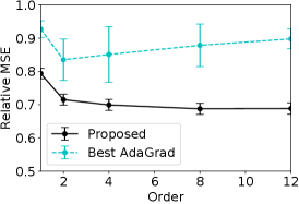
C.4 Details of the results from the experiments with stock indices

Figure 8-12 shows the results in Figure LABEL:fig:all with error bars. In each figure, the relative MSE of Algorithm LABEL:alg:adaptive and baselines are compared on a particular financial index. The baselines are vSGD, HGD, Almeida, Cogra, Adam, AdaGrad, and RMSProp, and each panel shows the relative MSE with one of the baselines. The figures also show error bars, which are computed on the basis of the standard deviation of the MSE on each of the 10 intervals of equal length.

The results with HGD, Almeida, and Cogra look similar to each other in the figure. This is because, for the financial time-series under consideration, the prediction by these three methods was quite close to the naive prediction that the absolute daily return stays unchanged from the previous day. Because we compute the error bars on the basis of the standard deviation of the MSE on each of the 10 intervals of equal length, the error bars of these three methods also look similar to each other.

References

Osogami [2021] T. Osogami. Second order techniques for learning time-series with structural breaks. In Proceedings of the 35th AAAI Conference on Artificial Intelligence (AAAI-21), 2021.