Prompt emission and early optical afterglow of VHE detected GRB 201015A and GRB 201216C: onset of the external forward shock
Abstract
We present a detailed prompt emission and early optical afterglow analysis of the two very high energy (VHE) detected bursts GRB 201015A and GRB 201216C, and their comparison with a subset of similar bursts. Time-resolved spectral analysis of multi-structured GRB 201216C using the Bayesian binning algorithm revealed that during the entire duration of the burst, the low energy spectral index () remained below the limit of the synchrotron line of death. However, statistically some of the bins supported the additional thermal component. Additionally, the evolution of spectral parameters showed that both peak energy () and tracked the flux. These results were further strengthened using the values of the physical parameters obtained by synchrotron modeling of the data. Our earliest optical observations of both bursts using FRAM-ORM and BOOTES robotic telescopes displayed a smooth bump in their early optical light curves, consistent with the onset of the afterglow due to synchrotron emission from an external forward shock. Using the observed optical peak, we constrained the initial bulk Lorentz factors of GRB 201015A and GRB 201216C to = 204 and = 310, respectively. The present early optical observations are the earliest known observations constraining outflow parameters and our analysis indicate that VHE-detected bursts could have a diverse range of observed luminosity within the detectable redshift range of present VHE facilities.
1 Introduction
Gamma-ray bursts (GRBs) are sudden intense explosions of electromagnetic radiation in the –MeV energy range, releasing energy () in the range of erg. GRBs emit radiation across the electromagnetic spectrum broadly into two successive phases, i.e., prompt emission (generally in gamma rays or hard X-ray band) and afterglow emission (from radio to gamma rays), respectively (Kumar & Zhang, 2015). These cosmic stellar explosions are traditionally classified into long (LGRBs) and short (SGRBs) depending on their observed prompt emission duration (Kouveliotou et al., 1993), which can be traced back to different progenitors. A massive star collapse under certain physical conditions, a “collapsar”, is expected to be the progenitor of LGRBs (Woosley, 1993; Hjorth et al., 2003). On the other hand, SGRBs are believed to originate from the merging of compact binaries like two neutron stars or a neutron star and a black hole (Perna & Belczynski, 2002; Abbott et al., 2017). However, recent discoveries of a few GRBs exhibiting hybrid properties from the collapse of massive stars (Ahumada et al., 2021) as well as from binary mergers (Rastinejad et al., 2022; Troja et al., 2022) challenge current understanding and provide valuable clues about the physical nature of progenitors of GRBs.
There are many open questions related to the physics behind the prompt emission of GRBs, such as their jet compositions, emission mechanisms, and emission radii (see Kumar & Zhang 2015; Pe’er 2015 for a review). To understand the jet compositions, there are two widely accepted scenarios: (1) baryonic-dominated hot fireball (Shemi & Piran, 1990), and (2) Poynting flux-dominated outflow (Zhang et al., 2018). In addition, there is also the possibility of a hybrid model that includes both components, Poynting flux outflow moving along with a hot fireball (Pe’er, 2015). For the emission mechanisms, there are two widely accepted scenarios: (1) synchrotron emission from a cooling population of particles (Burgess et al., 2020), and (2) thermal photospheric emission (Pe’er, 2015). Since the beginning of the GRB spectroscopy, prompt spectral analysis of a larger sample of BATSE GRBs suggests non-thermal dominance, and spectra are described by a smoothly connected power-law empirical function, known as the Band function (Band et al., 1993). The low energy spectral index of the Band function is widely used to understand the possible radiation process. However, some authors used the physical synchrotron modeling and suggested that it is a more accurate method to constrain the radiation physics rather than empirical fitting (Burgess et al., 2020; Oganesyan et al., 2019).
Contrary to those predicted within the framework of the external forward and reverse shock models (Sari et al., 1998; Sari & Piran, 1999), the early time broadband afterglow emission of some GRBs exhibit deviations from power-law behavior such as flares, bumps, and plateaus largely attributed to effects from the unknown central engine. The early optical afterglow light curve initially rises until the blast wave reaches the self-similar phase, and the bulk Lorentz factor remains almost constant to its initial value. When the light curve is at its peak, the blast wave carries enough matter for the bulk Lorentz factor to begin progressively decreasing following the self-similar solution (Blandford & McKee, 1976), which makes the light curve decay, a process known as the onset of afterglow (Sari & Piran, 1999). Sari & Piran (1999) explored the early optical afterglow emission and noted that the detection of the onset of afterglow can be utilized to calculate the initial bulk Lorentz factor of the relativistic outflow. Fast slewing (within a few minutes) of optical space (Swift Ultra-Violet and Optical Telescope) and ground-based telescopes (robotic telescopes such as MASTER, BOOTES, FRAM, etc.) are required to discover the onset of optical afterglow. Liang et al. (2010) carried out an extensive search for the onset signatures in the early afterglow and identified twenty GRBs (through the literature search up to 2009) with an initial bump in their optical light curves. Additionally, they studied correlations among the characteristic parameters of the optical bump, like peak time, FWHM, isotropic energy, etc., and noted that most of the parameters have strong correlations with each other.
In recent years, detections of very high energy gamma-ray emissions during the afterglow phase by the imaging atmospheric Cherenkov telescopes such as Major Atmospheric Gamma Imaging Cherenkov (MAGIC, MAGIC Collaboration et al. 2019a), High Energy Stereoscopic System (H.E.S.S., H.E.S.S. Collaboration et al. 2021), and Large High Altitude Air Shower Observatory (LHAASO, Huang et al. 2022) including the recently discovered GRB 221009A have challenged our understanding of afterglows and has opened a new window to explore this phase in more detail. A few general characteristics of VHE detected GRBs are tabulated in Table 1. Generally, the traditional synchrotron emission can not explain the spectral energy distributions (SEDs) of VHE detected bursts. The double bump features observed in the broadband SEDs of GRB 180720B and GRB 190114C demand a synchrotron emission mechanism for the first bump and synchrotron-self Compton (SSC) to account for the second bump (Abdalla et al., 2019; MAGIC Collaboration et al., 2019a). However, in the case of the nearby VHE detected GRB 190829A, the spectral index calculated using H.E.S.S. data was similar to the one of the synchrotron emission observed in the X-ray band, indicating that a single synchrotron component is sufficient to model the observed broadband spectrum from radio to VHE energies (H.E.S.S. Collaboration et al., 2021). In addition, in the case of GRB 190829A and GRB 190114C, dusty environments (large values of optical extinction in the host galaxies) have been observed, indicating a possible relationship between the occurrence of VHE emission and dusty environments (de Ugarte Postigo et al., 2020b; Zhang et al., 2021; Gupta et al., 2022a).
In this paper, we present a detailed prompt emission, and early optical afterglow analysis of two of the VHE detected bursts, GRB 201015A (Suda et al., 2022) and GRB 201216C (Fukami et al., 2022). The article has been organized in the following sections: § 2 presents multi-wavelength observations of GRB 201015A and GRB 201216C, followed by the prompt and afterglow data analysis. The main results are given in § 3, and followed by the discussion in § 4. Finally, the summary and conclusions are given in § 5. Unless otherwise stated, all the uncertainties are expressed in throughout this article. We consider the Hubble parameter , density parameters and .
| VHE detected GRBs | Light curve morphology | ( keV) | (erg) | (erg/s) | Ambient-medium | X-ray flare | Supernova connection | |
| 160821B(1,2) | Short and bright pulse | 0.162 | 8419 | 2.101050 | 2.001050 | ISM | No | kilonova |
| 180720B(3,4) | Single broad multi-peak light curve | 0.654 | 45149 | 6.001053 | 1.801053 | ISM | Yes | No |
| 190114C(5,6) | Bright multi-peak pulse followed by soft tail emission | 0.424 | 92617 | 2.501053 | 1.671053 | wind/ISM | No | Yes |
| 190829A(7,8) | Two-episodes with 40 s quiescent gap | 0.0785 | 11.50.4 | 3.001050 | 3.001049 | ISM | Yes | Yes |
| 201015A | Short overlapping pulses followed by soft and weak tail | 0.426 | 4114 | 3.861051 | 3.861050 | ISM | No | Yes |
| 201216C | Complex multi-pulsed structured light curve | 1.1 | 35212 | 6.321053 | 8.781052 | wind | No | No |
| 221009A(9,10,11,12,13) | Two emission episodes followed by a long tail, extraordinarily brightness | 0.151 | 1060 30 | 3 1054 | 1 1052 | wind | No | Yes |
2 Multi-wavelength Observations and data reduction
In the present section, we report the prompt emission, afterglow observations and data reduction of GRB 201015A and GRB 201216C taken from space and ground-based facilities and are part of the present analysis.
2.1 Prompt gamma-ray observations
The Burst Alert Telescope (BAT, Barthelmy et al. 2005) onboard the Neil Gehrels Swift observatory (henceforth Swift) triggered GRB 201015A at 22:50:13.00 UT on 2020 October 15 (T0) with a total duration of 10 s in the 15-350 keV energy range. The burst was localized to RA, Dec = 354.310, +53.446 degrees (J2000) with a BAT uncertainty circle of 2.9′ (D’Elia et al., 2020). At the time of Swift detection, the Gamma-ray Burst Monitor (GBM, Meegan et al. 2009) onboard Fermi was observing the field of view of the GRB, but was unable to trigger on the burst. However, the burst was identified in GBM data through a targeted search from 30 s around the Swift-BAT trigger time.
The Fermi-GBM triggered GRB 201216C at 23:07:25.75 UT on 2020 December 16 (T0, Malacaria et al. 2020). At T0, the burst location was outside the field of view (FoV) of the Large Area Telescope (LAT) onboard Fermi (boresight angle is 93.0 degrees). It came into the FoV of LAT at T0 +3500 s and remained visible until T0 +5500 s. However, no significant GeV emission associated with GRB 201216C was observed during this time window (Bissaldi et al., 2020). In addition to Fermi, the Swift-BAT triggered GRB 201216C at 23:07:31.00 UT on 2020 December 16 with a T90 duration of 48.0 16.0 s in the 15-350 keV range (Beardmore et al., 2020; Ukwatta et al., 2020). The burst was localized at RA, Dec = 16.358, +16.537 degrees (J2000) with a BAT uncertainty circle of radius 3 arcmin (Beardmore et al., 2020). The prompt emission of GRB 201216C was also detected by AstroSat CZT-Imager (Nadella et al., 2020) and Konus-Wind (Frederiks et al., 2020).
Swift-BAT data analysis: We retrieved the Swift-BAT observation data for both the bursts from their Swift archive pages (GRB 201015A, obsID: 01000452000 and GRB 201216C, obsID: 01013243000111https://www.swift.ac.uk/archive/selectseq.php?tid=01013243&source=obs), respectively. We performed general processing of the BAT data given in the Swift-BAT Software Guide222https://swift.gsfc.nasa.gov/analysis/bat_swguide_v6_3.pdf. Further, we analyzed the standard temporal and spectral BAT data products following the BAT data analysis methods given in Gupta et al. (2021b); Caballero-García et al. (2022). In this work, we have utilized the Multi-Mission Maximum Likelihood framework (Vianello et al., 2015, 3ML333https://threeml.readthedocs.io/en/latest/) software for the time-averaged spectral analysis. We considered the BAT spectrum over the 15-2022MNRAS.511.1694G150 keV energy range for the spectral analysis of the BAT data.
Fermi-GBM data analysis: For the Fermi-GBM data analysis of GRB 201216C, we downloaded the GBM time-tagged events (TTE) mode data from the Fermi-GBM Burst Catalog444https://heasarc.gsfc.nasa.gov/W3Browse/fermi/fermigbrst.html. We selected the three brightest sodium iodide (NaI) and brightest bismuth germanate (BGO) detectors with minimum observing angles for temporal and spectral analysis of GBM data. We followed the methodology given in Caballero-García et al. (2022); Gupta et al. (2022b) for the spectral and temporal analysis of Fermi-GBM data.
In this work, we have utilized 3ML (Vianello et al., 2015) software for the time-averaged and time-resolved555For GRB 201015A, we could not perform the time-resolved spectral analysis as Fermi (having broad spectral coverage) was unable to trigger on the burst. spectral analysis. We considered the GBM spectrum over 8-900 keV (NaI detectors) and 200-40000 keV (BGO detector) energy ranges. We initially used two empirical models, Band and Cutoff power-law (CPL), to fit the time-averaged spectrum. To find the best fit model among the empirical models, we compared the deviance information criterion (DIC) values and chose the best model with the least DIC value ( DIC -10). Furthermore, we checked whether the addition of a thermal component (Blackbody) with Band, or Cutoff power-law in the spectrum improves the fitting or not. We have applied the following criterion to determine if the spectrum has a thermal component:
DICDICDICBand/CPL
The negative value of DIC suggests an improvement in the spectral fit. If the difference in DIC is less than -10, it shows the existence of a significant amount of thermal component in the spectrum.
Burgess et al. (2020) suggested that the empirical models may not be able to reveal the emission process of GRBs. They found that GRB spectra can be well modeled with a physical synchrotron model even if the low-energy spectral index of the same spectra exceeds the synchrotron line-of-death if modeled using a Band model. Therefore, in addition to empirical models, we have also used the physical synchrotron to model the emission mechanism of GRB 201216C. In this article, we have used the same physical synchrotron model pynchrotron666https://github.com/grburgess/pynchrotron (synchrotron emission from cooling electrons) for the spectral modeling of GRB 201216C used in Burgess et al. (2020). The synchrotron model is based on a comprehensive electron acceleration mechanism assumption. According to that, electrons are continuously injected into a power-law spectrum: N() with , where is the spectral index of the injected electrons, and are the lower and upper boundary of the injected electron spectrum, respectively. The cool synchrotron physical model details have been explained in Burgess et al. (2020). This model is characterized by the six physical parameters: 1. Magnetic field strength (B), 2. Spectral index of electrons (), 3. , 4. , 5. Characteristic Lorentz factor corresponds to the electrons’ cooling time (), and 6. Bulk Lorentz factor ().
During the spectral modeling, we fixed some of the physical parameters. We have fixed = 105 due to a strong degeneracy between magnetic field strength and . The bulk Lorentz factor () is fixed at 513, obtained using the onset of optical afterglow (see § 3.2.2). Furthermore, we have fixed = 108 since the fast cooling synchrotron physical model does not fit the prompt spectrum of GRBs well (Burgess et al., 2020).
Time-resolved spectral analysis of GRB 201216C: The time-resolved spectral analysis of the prompt emission using broad spectral coverage GRB detectors such as Fermi-GBM has been used as a promising tool to investigate the emission mechanism and to study the correlations between the spectral parameters of GRBs. To constrain the radiation process and spectral evolution of GRB 201216C, we performed the time-resolved spectral analysis using 3ML software with the same number of detectors used for the time-averaged spectral analysis. 3ML provides four possible methods to bin the light curves of GRBs. 1. Constant cadence (Cc) binning. All bins are equally spaced with the initially chosen time-width T. One disadvantage is that the spectral shape may vary slower or faster than the specified cadence. 2. Signal-to-noise (S/N) binning: here, we predefined the S/N for each bin, which ensures enough photons in each time bin, but it may fail to recover the intrinsic spectral evolution behavior of GRBs, 3. Knuth binning, and 4. Bayesian Blocks binning, in this case, the time bins have unequal widths and a variable signal-to-noise ratio. Burgess (2014) studied all these methods and suggested that the Bayesian Block binning method is the best time-slicing method to correctly obtain the intrinsic spectral evolution of GRBs. However, this method has one limitation: some bins might not have enough photons needed for correct spectral modeling. In the case of GRB 201216C, we initially performed the Bayesian Block binning on the brightest GBM detector (energy range 8–900 keV) considering the false alarm probability P = 0.01 (Scargle et al., 2013), and the other GBM detectors used the same temporal binning information. This results in 37 time-sliced spectra for time-resolved analysis of GRB 201216C. Further, we measured each spectrum’s statistical significance (S, Vianello 2018) to ensure enough photon counts for spectral analysis and considered temporal bins with statistical significance greater than 25. This results in 27 time-sliced (Bayesian Block) spectra with S 25.
For the time-resolved spectral analysis of GRB 201216C, we initially used the empirical Band and Cutoff power-law models and then refitted each spectrum after adding a thermal component to the empirical models. Furthermore, we fitted each spectrum using the physical slow cooling Synchrotron model. We have used the Bayesian fitting method for the spectral fitting, and the sampler is set to the multi-nest with 10,000 iterations. The spectral parameters, along with the associated errors, obtained using the time-resolved spectral analysis of GRB 201216C using the empirical and physical models are given in Table 5, 6 and 7 of the appendix.
2.2 Afterglow observations
The afterglows of GRB 201015A 777https://gcn.gsfc.nasa.gov/other/201015A.gcn3 and GRB 201216C 888https://gcn.gsfc.nasa.gov/other/201216C.gcn3 were discovered from VHE to radio wavelengths by various observational facilities over the globe, including our earliest optical afterglow observations using the robotic telescopes, FRAM-ORM (Jelinek et al., 2020a, b) and BOOTES (Hu et al., 2020). The redshifts of GRB 201015A ( = 0.426) and GRB 201216C ( = 1.1) were measured using spectroscopic observations (emission features) of 10.4m GTC (de Ugarte Postigo et al., 2020a) and the Very Large Telescope (Vielfaure et al., 2020), respectively. The redshift measurement of GRB 201216C places the burst as the most distant known source associated with VHE emission (see Table 1).
2.2.1 X-ray afterglows
For GRB 201015A, Swift could not slew until T0 +51.6 minutes due to an observing constraint (D’Elia et al., 2020). The Swift X-ray telescope (XRT, Burrows et al. 2005) began observations of GRB 201015A at 23:43:47.2 UT on 2020 October 15, 3214.1 s post burst. Swift-XRT detected an uncatalogued fading X-ray source at the following location: RA, Dec = 354.32067, +53.41460 degrees (J2000) with an uncertainty radius of 3.8" (Kennea et al., 2020). Swift-XRT observed this source up to ks after the BAT detection. All observations were obtained in Photon Counting (PC) mode.
For GRB 201216C, Swift-XRT began observations at 23:56:58.5 UT on 2020 Dec 16, 2966.8 s post burst. Swift-XRT detected a new fading X-ray source at the following location: RA, Dec = 16.37114, +16.51659 degrees (J2000) with an uncertainty circle of 3.5" (Campana et al., 2020). Swift-XRT observed this source up to 2.2 ks after the initial detection. Window timing (WT) mode was used for the first 25 s of observations, and the remaining observations were obtained in PC mode.
X-ray afterglow data analysis: In this work, we obtained the Swift-XRT data products from the XRT repository provided by the University of Leicester (Evans et al., 2007, 2009). We modeled the X-ray afterglow light curves of both the bursts using power-law and broken power-law empirical models to constrain their decay rates. On the other hand, to constrain the spectral indices, we modeled the XRT spectra of both the bursts in the energy range of 0.3-10 keV using the X-ray Spectral Fitting Package (XSPEC; Arnaud, 1996). We fixed the Galactic hydrogen column density to be = , and cm-2 for GRB 201015A and GRB 201216C, respectively (Willingale et al., 2013). A more detailed method for the standard temporal and spectral XRT analysis is given in Gupta et al. (2021b).
2.2.2 Optical afterglows of GRB 201015A and GRB 201216C
GRB 201015A: The optical afterglow of GRB 201015A was first reported by the MASTER robotic telescope at the position RA= 23:37:16.42, DEC= +53:24:55.8 (Lipunov et al., 2020). In this paper, we present our optical observations from the 25cm FRAM-ORM (Jelinek et al., 2020a), Burst Observer and Optical Transient Exploring System (BOOTES) (Hu et al., 2020), and 3.6m Devasthal Optical Telescope (DOT), along with additional optical data from the GCN circulars. Our photometric observations are listed in Table LABEL:table:15A_optical of the appendix.
BOOTES-network: The BOOTES-network followed GRB 201015A with three robotic telescopes at BOOTES-1 (INTA-CEDEA) station in Mazagon (Huelva, Spain) and BOOTES-2/TELMA station in La Mayora (Malaga, Spain). The BOOTES-1B performed one epoch of early observations at 22:50:48 on 2020 October 15, and the afterglow is clearly seen in the images. The BOOTES-1A performed two epoch observations: the first was the quick follow-up to the trigger and the second was the late follow-up on the next day. The BOOTES-2/TELMA also followed this event on 2020-10-16T22:15:13. The afterglow was not visible in both BOOTES-1A’s and BOOTES-2’s images.
A series of images were obtained with BOOTES-1B robotic telescope in the clear filter with exposures of 1 s, 10 s, and 60 s for GRB 201015A. The image preprocessing (bias and dark-subtracted, flat-fielded, and cosmic-ray removal) was done using custom IRAF routines. The photometry was carried out using the standard IRAF package. The images were calibrated with nearby comparison stars from the Pan-STARRS catalog, which were imputed to R-band through the transformation equation from Lupton (2005)999http://www.sdss.org/dr12/algoritms/sdssUBVRITransform/ for the data in the clear filter. The obtained magnitudes are listed in Table LABEL:table:15A_optical of the appendix.
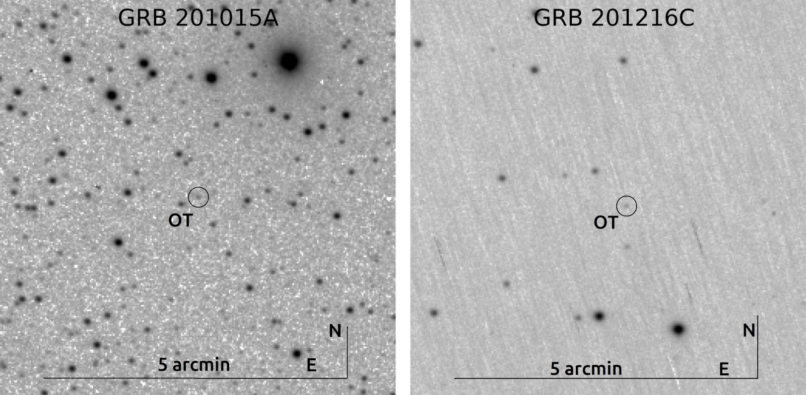
FRAM-ORM: The FRAM-ORM is a 25cm f/6.3 robotic telescope facilitated with B, V, R, and z filters and a custom Moravian Instruments G2-1000B1 camera based on a back-illuminated CCD47-10 chip. We carried out the earliest optical observations of GRB 201015A using the 25cm FRAM-ORM robotic telescope located at La Palma, Spain. We obtained a series of frames with exposure times of 20 s each in the clear filter, beginning on 2020 October 15 at 22:50:50.8 UT (37.6 s after the BAT trigger). We have clearly identified the source mentioned by Lipunov et al. (2020). A finding chart of FRAM-ORM observation of GRB 201015A is given in Figure 1.
3.6m DOT: We performed the optical observations of the afterglow of GRB 201015A starting on 2020 October 16 at 13:09:07.2 UT ( 0.6 days post burst) using 3.6m DOT located at the Devasthal observatory, which is part of the Aryabhatta Research Institute of Observational Sciences (ARIES), India. We acquired multiple frames in B, V, R, and I filters (with an exposure time of 10 minutes in each) using the 4K 4K CCD IMAGER (Kumar et al., 2022b) mounted on the main port of 3.6m DOT. In stacked DOT images, we clearly detect the optical afterglow of GRB 201015A consistent with the error region of NOT observations Malesani et al. (2020). A finding chart of 3.6m DOT observation of GRB 201015A is given in Figure 15 of the appendix. We performed the DOT image reduction using the IRAF package. We first applied zero correction and flat fielding to the raw images taken from the telescope. After the removal of cosmic-ray hits, we stack the images to create a single image. We use the IRAF package to perform the aperture photometry. For the photometric calibration of GRB 201015A, standard stars in the Landolt standard field PG 0231 were observed along with the GRB field in UBVRI bands. The R-band finding chart of GRB 201015A and the secondary stars marked with S1-S14 are shown in the Figure 15. The calibrated magnitudes of secondary stars are listed in Table 10 of the appendix, and the calibrated magnitudes of GRB 201015A are listed in Table LABEL:table:15A_optical of the appendix.
GRB 201216C: In the case of GRB 201216C, Izzo et al. (2020) carried out the optical follow-up observations in the Sloan g, r, z filters using VLT telescope, starting at 01:18:47 UT on 2020 December 17. They first reported the detection of an uncatalogued optical source at location RA: 01:05:28.980, Dec: +16:31:00.0 (J2000.0), consistent with the Swift-XRT enhanced location (Campana et al., 2020).
FRAM-ORM: We performed the earliest optical follow-up observations to the alert of GRB 201216C using the FRAM-ORM telescope. We obtained a series of frames with an exposure times of 20 s each in the clear filter, starting on 2020 December 16 at 23:08:04.3 UT (31.6 s after the BAT trigger) (Jelinek et al., 2020b). We immediately detected an optical transient consistent with the location reported by Izzo et al. (2020). A finding chart of FRAM-ORM observation of GRB 201216C is given in Figure 1. A log of photometric observations of the afterglow of GRB 201216C is presented in Table 12 of the appendix.
The observed frames for both the bursts have been processed through a difference imaging pipeline based on the HOTPANTS image subtraction code to remove the influence of nearby stars on the photometric measurements and then corrected for bias, flats, and cosmic-rays. The photometry has been carried out using the DAOPHOT package. The measured magnitudes have been calibrated using field stars in the PanSTARS DR1 catalog. Our optical observations reveal an early rise in the light curves of both bursts, reaching their maximum and followed by normal decay until the end of our observations. A log of our photometric observations is given in Table LABEL:table:15A_optical of the appendix.
3 Results
3.1 Prompt emission
In this section, we present the results of comprehensive analysis of prompt emission of GRB 201015A and GRB 201216C. We have summarized our results in Table 2.
3.1.1 Light curve and time-averaged spectra
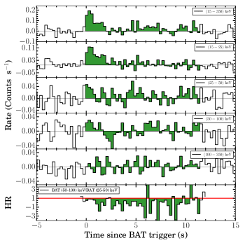
The Swift-BAT energy-resolved mask-weighted light curve of GRB 201015A along with HR evolution in 25-50 keV and 50-100 keV energy range is shown in the top panel of Figure 2. The Swift-BAT prompt emission light curve of GRB 201015A has a short-soft emission starting from T0 and ending at T0 +1 s, followed by a weak-soft tail emission that lasts till T0 +10 s (Markwardt et al., 2020). The time-integrated spectrum (T0-0.21 to T0 +11.57 s) of GRB 201015A is explained using the simple power-law model with power index = -2.43 0.25 (see Figure 8 of the appendix).
| Properties | GRB 201015A | GRB 201216C |
|---|---|---|
| T90 (s) | 9.78 3.47 | 29.95 0.57 |
| HR | 0.72 | 1.11 |
| ( keV) | 41.37 | 352.31 |
| Fluence (erg ) | ||
| (erg) | 3.86 | |
| (erg/s) | 3.86 | 8.78 |
| 0.426 | 1.1 | |
| SN association | Yes | No |
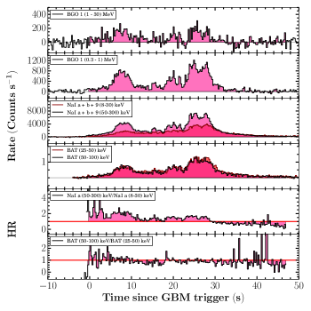
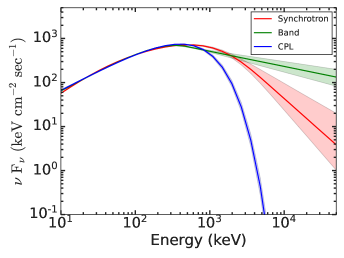
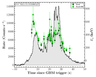
The background-subtracted energy-resolved Fermi-GBM light curve of GRB 201216C along with the hardness-ratio (HR) evolution is shown in the bottom panel of Figure 2. The Fermi-GBM prompt emission light curve consists of a broad, structured peak with a T90 duration of 29.9 s (in 50-300 keV). Similar to the Fermi-GBM, Swift-BAT observations also reveal multiple peaks in the mask-weighted prompt light curve. According to BAT observations, the energy fluence of the burst is 4.5 erg in the 15-150 keV energy range (Ukwatta et al., 2020). Figure 2 also shows the time interval used for the time-averaged spectral analysis. The time-averaged Fermi-GBM spectrum (from T0-0.503 s to T0 +47.09 s) is best modeled using a Band+BB function (see Figure 8 of the appendix) and the best fit spectral parameters are presented in Table 4 of the appendix. The burst was significantly bright: the observed fluence is (2.00 0.10) erg in the 10-104 keV energy band over the time-averaged interval. This fluence value is among the top 2 percent of the brightest GRBs observed by Fermi-GBM. A comparison between the time-averaged energy spectrum of the empirical (Band, CPL) and physical (Synchrotron) models are shown in Figure 3.
3.1.2 Time-integrated T90-Spectral hardness distribution
GRBs are classified into two families based on T90 duration, however, there is one more fundamental difference between both the classes, i.e., spectral hardness. Long GRBs are expected to be softer (lower value), on the other hand, short bursts are usually harder (higher value). To know the true class of GRB 201015A and GRB 201216C, we placed both bursts in the time-integrated T90-spectral hardness plane along with the other long and short GRBs obtained from the Fermi-GBM and Swift-BAT catalogs.
We calculated the hardness ratio (HR) for GRB 201015A using the ratio of fluence in hard (50-100 keV) and soft (25-50 keV) energy ranges and found its value equal to 0.72. Comparing the HR of GRB 201015A with the Swift-BAT catalog, we note that GRB 201015A is one of the softest bursts ever observed by the Swift mission (see Figure 9 of the appendix). In the case of GRB 201216C, we calculated the HR using the ratio of counts in hard (50-300 keV) and soft (8-30 keV) energy ranges to be 1.11, this feature is similar to long/soft GRBs. The distribution of HR as a function of T90 for both the bursts are given in Figure 9 of the appendix.
Furthermore, we also placed both the bursts in the time-integrated -T90 distribution of long and short GRBs. As for GRB 201015A there was no onboard observation by Fermi and no public Fermi data is available for ground targeted search, we have used Swift-BAT observations of GRB 201015A to constrain the time-integrated peak energy. However, the BAT time-integrated spectra of GRBs are usually modeled by simple power-law functions due to the instrument limited spectral coverage (15-150 keV). In the case of GRB 201015A, the time-integrated spectrum is also fitted using a power-law function (see § 3.1.1). We estimated the value using the known correlation between the Swift-BAT fluence and time-integrated (Zhang et al., 2020), i.e., = [fluence/()]0.28 keV 41.37 keV. The estimated time-integrated value of GRB 201015A is consistent with those observed for long GRBs. In the case of GRB 201216C, we fitted the time-integrated spectrum and calculated the peak energy ( = 352.31 keV) using the best fit model. The T90- distribution for both the GRBs is shown in Figure 9 of the appendix along with other data points obtained from Fermi-GBM catalog (Goldstein et al., 2017). We fitted the complete distribution obtained from Fermi-GBM catalog using the Bayesian Gaussian mixture model (BGMM) algorithm and calculated the probability of GRB 201216C being a long burst as 98.8 %.
3.1.3 Prompt correlations: Amati and Yonetoku
The cosmological corrected time-integrated peak energy = (1+z) of the prompt emission is correlated with the isotropic equivalent energy , and isotropic peak luminosity . The former is known as Amati correlation (Amati, 2006) and the later is known as Yonetoku correlation (Yonetoku et al., 2004). In the case of GRB 201015A, we have used equation 6 of Fong et al. (2015) to calculate due to the limitation of Swift-BAT spectral coverage. On the other hand, we have used the best fit Fermi-GBM time-integrated spectral model to calculate the for GRB 201216C. The Amati correlation for both the GRBs along with a sample of long and short GRBs taken from Minaev & Pozanenko (2020) is presented in Figure 9 of the appendix. Similarly, we calculated the values and placed GRB 201015A and GRB 201216C in the - plane, as shown in Figure 9 of the appendix. We noticed that both the bursts satisfied the Amati and Yonetoku correlations. The calculated isotropic equivalent luminosity values for both the bursts suggest that GRB 201015A is an intermediate luminous GRB; on the other hand, GRB 201216C is a luminous GRB.
3.1.4 Time-resolved spectroscopy of GRB 201216C
Distribution of spectral parameters:
The mean values and standard deviation for each spectral parameter obtained using Cutoff power-law, Band, Cutoff power-law + BB, Band+ BB and Synchrotron models are listed in Table 8 of the appendix.
The mean values of the low energy spectral indices obtained using Cutoff power-law and obtained using Band spectral modeling of GRB 201216C are and , respectively. These values are consistent with the typical average value of the low energy spectral index ( ) of GRBs (Preece et al., 2000). Similarly, the averaged value of spectral peak energy and high energy photon index obtained using Band are keV, and , respectively. These values are also consistent with the typical average value of and of GRBs. The averaged values of physical synchrotron spectral parameters for GRB 201216C are following: magnetic field (B) = G, index (p) = , and Lorentz factor corresponds to the electron’s cooling time = .
Evidence for thermal component: In our time-resolved spectral analysis, we first fitted each binned spectra using empirical Band and Cutoff power-law models individually. To search for the presence of an additional thermal component in the spectrum, we added the Blackbody model along with Band and Cutoff power-law models, and calculated the difference of the DIC values. Negative values of and , implies that the additional Blackbody component improves the fit statistic. Furthermore, in the case of any particular bin, if , it suggests a significant amount of thermal component present in that particular bin. Figure 10 of the appendix shows the evolution of within the burst interval for Band + Blackbody model. For all the bins (except the last bin), values are negative, indicating that the addition of thermal components improves the spectral fitting. There are 10 bins ( 37 %) for which , suggesting for presence of thermal component in the spectrum. In light of this, we suggest that GRB 201216C is a hybrid (non-thermal+ quasi-thermal) burst. The thermal components are dominating during the initial and bright phases of the burst.
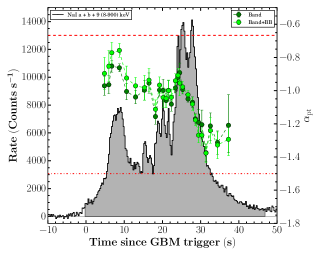
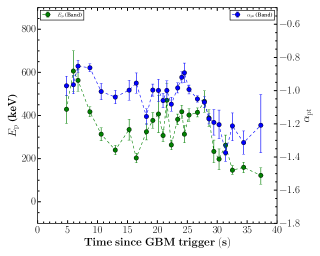
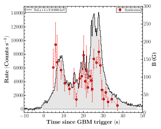
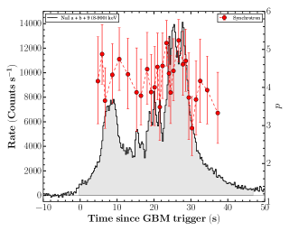
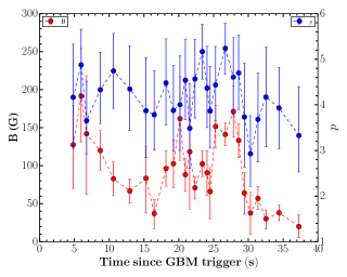
The evolution of spectral parameters: The studies of spectral evolution are a very powerful tool to probe the emission process responsible for the prompt emission. The peak energy of the Band function shows four different possible types of spectral evolution. 1. Hard to soft pattern (Norris et al., 1986), 2. Soft to hard pattern (Kargatis et al., 1994), 3. flux tracking pattern (Golenetskii et al., 1983) and 4. Chaotic pattern. On the other hand, the low energy spectral index of the Band function also changes with time, however, it does not show any particular trend. There are some recent studies suggesting a flux tracking pattern of , supporting the double tracking trend (Li et al., 2019). However, most of the spectral evolution studies are performed for single pulsed bursts. The prompt light curve of GRB 201216C shows a more complex multi-pulsed structure, and the evolution of empirical and physical spectral parameters are very interesting. Figure 4 shows the evolution of the spectral parameters (, and ) of GRB 201216C obtained using empirical Band function. The evolution of of GRB 201216C shows a flux tracking trend, i.e., increases and decrease as flux increases and decrease in respective bins. We noticed that the values are changing with time and do not exceed the expected values of spectral indices of synchrotron fast and slow cooling cases. We have also shown the evolution of and together in Figure 4, and we can see that the evolution patterns are quite similar throughout the emission. Next, we study the spectral evolution of parameters obtained from the physical synchrotron modeling. Figure 5 shows spectral evolution of the magnetic field strength (B), and spectral index of electrons (). We noticed that the magnetic field strength is also following the intensity of the burst. We could not confirm the evolution trend of due to large associated errors. In light of the above, we suggest that multi-pulsed GRB 201216C have flux tracking characteristics. We further investigated the correlation among these spectral parameters.
Spectral parameters correlations: Studying the correlations between the different spectral parameters obtained using the time-resolved spectral analysis using empirical and physical modeling gives an important clue about the physics of GRBs and jet composition. We calculated the correlation between Band and Band+Blackbody spectral parameters: log (Flux) and log (), log (Flux) and , log () and , and log (Flux) and k. We found a high degree (the correlation coefficient ranges from 0.60-0.79) of correlation between the Band spectral parameters, i.e., log (Flux) and log (), log (Flux) and , and log () and . We also found a high degree of correlation between log (Flux) and k for the Band+ Blackbody model. The correlation results for the Band and Band+ Blackbody models (Pearson correlation) are listed in Table 9 and Figure 11 of the appendix. We also studied the correlation between physical spectral parameters (log (Flux)-log (B), log (Flux)-, and log (B)-) obtained using Synchrotron model. We found a very high degree (the correlation coefficient is 0.80) of correlation between log (Flux)-log (B) and medium correlation (the correlation coefficient ranges from 0.40-0.59) between log (B)-, however, we found a low degree (the correlation coefficient ranges from 0.20-0.39) of correlation between log (Flux)-. The correlation results obtained using physical modeling are shown in Figure 12 and in Table 9 of the appendix.
In addition, we also studied the correlation between empirical and physical models parameters: log (B)-log (), log (B)-, and -. The correlation results are shown in Figure 13 and Table 9 of the appendix. We found a very high degree of correlation between log (B) of physical synchrotron model and log () of empirical Band function. We also found a medium degree of correlation between log (B) and , however, there is a low degree of correlation between and .
3.2 Afterglow emission of GRB 201015A and GRB 201216C:
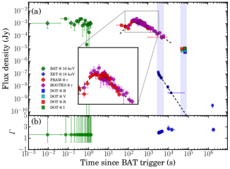
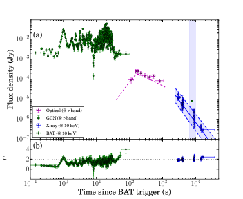
In the present section, we study the results of multi-wavelength afterglow of GRB 201015A and GRB 201216C, detected by Swift-XRT (X-ray), FRAM-ORM, BOOTES and 3.6m DOT (optical). Multi-wavelength light curves of GRB 201015A and GRB 201216C are shown in Figure 6, whereas SEDs are discussed in Figure 7.
3.2.1 X-ray afterglows
The X-ray afterglow light curves of GRB 201015A and GRB 201216C do not show any flare, bump, break, or plateau-like activities (see Figure 6).
In the case of GRB 201015A, we initially tried to fit the X-ray light curve using a simple power-law model (temporal index = -2.36). The calculated XRT temporal index is consistent with the temporal index reported on the XRT catalogue page using count rate light curve fitting101010https://www.swift.ac.uk/xrt_live_cat/01000452/. However, the model shows a significant deviation from the last observed data point (chi/dof =1.34). We noted that the last two data points are considered unreliable because no centroid could be determined. We calculated the XRT temporal decay index = -2.27 excluding these points. We found that both the calculated XRT decay indices are consistent, considering the large associated errors. We also used the broken power-law function to fit the light curve and obtained chi/dof = 0.27, indicating that the model is over fitting the data. Further, we used F-test to find the best fit model among the two empirical models. The F-test suggests that the simple power-law model is better fitting the X-ray afterglow light curve of GRB 201015A, consistent with those reported on the XRT catalogue page. The X-ray light curve and the best fit model are shown in Figure 6. For the XRT spectral analysis, we fitted the late time spectrum (T0 +4000 to T0 +22019 s) to constrain the intrinsic hydrogen column density () of GRB 201015A and calculated = cm-2. The time-averaged X-ray spectrum (T0 +3300 to T0 +1800000 s) of GRB 201015A is described using an absorbed power-law model with a spectral index = 1.10. Further, we divided the XRT light curve into three segments based on available observations. For the first (T0 +3300 to T0 +4800 s), second (T0 +10000 to T0 +15000 s), third (T0 +10000 to T0 +1800000 s) time bins, we obtained the spectral indices = 1.07, 1.10, and 1.38, respectively. Our analysis does not find any noticeable evolution among the spectral indices within the observed duration considering large values of associated errors.
The X-ray light curve of GRB 201216C is shown in Figure 6. The light curve (@ 10 keV) decay as a power-law with a decay index of = with (chi/dof =3.35). For the XRT spectral analysis, we calculated the of the host using the late time spectral fitting (T0 +4001 to T0 +37346 s) and found = cm-2. The joint PC and WT mode time-averaged X-ray spectrum (T0 +2900 to T0 +17000 s) of GRB 201216C is described using an absorbed power-law model with a spectral index = 0.97. Further, we created the spectrum for individually segmented WT and PC mode observations using the Swift Science Data Centre web-page111111https://www.swift.ac.uk/xrt_spectra/addspec.php?targ=01013243&origin=GRB and performed the spectral fitting. For the WT (T0 +2900 to T0 +3000 s), and PC (T0 +3300 to T0 +17000 s) time bins, we obtained the spectral indices = 0.87, and 0.90, respectively. Our analysis indicates that the spectral index is not changing with time (see Figure 6).
3.2.2 Optical afterglows
For both these VHE detected bursts, we can examine the early afterglow behavior using the earliest optical observations from the 0.25m robotic FRAM-ORM and BOOTES telescopes (Jelinek et al., 2020a, b; Hu et al., 2020).
The optical light curve of GRB 201015A is highly rich in features. Following an early decay, the light curve has a smooth optical bump, which may be either due to reverse shock emission or the onset of afterglow in the forward shock. We calculated the decay rate for the very early optical emission . To characterize the nature of the early bump, we fitted the optical bump using a smoothly broken power-law function, given in equation 1.
| (1) |
Where and are the rise and decay temporal indices, respectively. is the normalization constant, and is the break time. The break time is related to the observed peak time () by the following equation:
| (2) |
In the case of GRB 201015A, the smoothly broken power-law fit (smoothness parameter ) shows that initially, the optical afterglow light curve rises with a temporal index of =1.74 and then decays with an index of =1.10, with the break time =217.04 s post burst. Further, we obtained the peak time = 184.64 s post burst using equation 2.
In the case of GRB 201216C, our early optical observations with FRAM-ORM telescope reveals a smooth bump in the optical afterglow light curve. We fitted the optical bump using the smoothly broken power-law function (see equation 1) and calculated the following temporal parameters: rising temporal index =, decay temporal index =, and the break time = s post burst, respectively. Further, we determine the peak time = 179.90 s post burst using the equation 2 (smoothness parameter = 3).
Reverse shock origin: According to the fireball model, the forward (moving towards the external/surrounding medium), and the reverse (propagating into the blast wave) shocks are originated due to the results of external shock between the blast-wave and ambient medium. The observed early optical peak in the afterglow light curve might be created due to the reverse shock (Kobayashi & Zhang, 2003). We used the expected temporal indices (for ISM and wind mediums in the thin and thick shells reverse shock cases) to determine the origin of early optical bump for both bursts (see Table 1 of Gao et al. (2015)). We note that the observed temporal indices values during the rising and decaying part of the bump of both the bursts are inconsistent with the expected values from the reverse shock decay in ISM or wind mediums. Therefore, the observed early bump in the optical light curves could not be due to the reverse shock.
Onset of optical afterglow: The early peak in the afterglow light curve can be produced by the onset of the afterglow and it can be used to calculate the the bulk Lorentz factor of the fireball (Sari & Piran, 1999). Ghirlanda et al. (2018) examined the early temporal coverage of GRBs with a measured redshift and calculated the bulk Lorentz factor for 67 bursts using the peak of the afterglow. In addition, they also summarize the methods used by various authors to estimate the bulk Lorentz factor. In the case of thin shell regime (T90 is less than deceleration time), the peak time (in the rest frame) of the light curve provides a direct measurement of the deceleration time . At the deceleration time, the Lorentz factor diminishes by a factor of two from its initial value () and enters into the self-similar deceleration phase. For the homogeneous medium surrounding the burst, the thin shell deceleration time is related to deceleration radius and bulk Lorentz factor with the following relation (Sari & Piran, 1999; Molinari et al., 2007):
| (3) |
Further, Ghirlanda et al. (2018) generalized the relation for both types of the surrounding medium (see equation 4).
| (4) |
Where s = 0 and K = 1.702 for ISM, and s = 2 and K = 1.543 for the wind-like ambient medium. is the isotropic equivalent -ray energy, is the proton mass, is the circumburst medium density, and is the radiative efficiency of the fireball.
The optical light curve of both GRB 201015A and GRB 201216C has a smooth bump that is well separated from the prompt emission, implying that the emission is in the thin shell regime. For the present analysis, we consider equal to 0.2 for both types of ambient medium. Further, we assume the value of = 1 cm-3 for ISM medium. The wind medium circumburst profile is governed by the mass loss rate and wind velocity . Therefore, we used = cm-3 for wind medium (Ghirlanda et al., 2018). To determine the bulk Lorentz factor using the early bump, we have used the methodology described by (Molinari et al. 2007, hereafter M2007).
3.2.3 Spectral energy distributions and closure relation
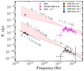
We created the SEDs using joint X-ray and optical data for both the bursts to constrain the break frequencies of the broadband synchrotron model at two epochs for GRB 201015A and one epoch for GRB 201216C, respectively. We followed the methodology given in Hu et al. (2021); Caballero-García et al. (2022); Gupta et al. (2022c) to create these SEDs. For GRB 201015A, the optical temporal index (=) follows a simple power-law decay post optical bump and satisfies the relation in the slow cooling regime of the ISM medium, which indicates that the optical emission always remains in the spectral regime. The details of epochs and temporal/spectral indices are given in Table 13 of the appendix. For GRB 201015A, we performed follow-up observations with 3.6m DOT in the BVRI filters. Our 3.6m DOT optical observations covering the temporal window from 52 ks–74 ks post burst are shown in Figure 7. We created an optical SED to calculate the optical spectral index and constrain the spectral regime at the epoch of DOT observations. The magnitudes are corrected for galactic extinction. In addition, we used negligible host extinction from Giarratana et al. (2022), and fitted a power-law function to determine the optical spectral index . We obtained a value of =-1.130.30. The calculated value of using DOT observations is shallower than (0.3) the X-ray spectral index (=-1.38) at this epoch. The measured change in the spectral indices of optical and X-ray data indicates that the cooling frequency lies in between the optical and X-ray spectral regime, although large associated errors due to limited data points and it is hard to discard other possibilities as and are consistent within 1 sigma. We noted that an ISM-type surrounding medium and spectral regime is also favored by the afterglow modeling of GRB 201015A by Giarratana et al. (2022) at this epoch, although, they mainly use the preliminary optical magnitudes reported in various circulars. Using the calculated value of , we determined the power-law index of electron distribution = (2 + 1) = 3.26 0.60 at this epoch.
For GRB 201015A, we create optical-X-ray SED at two different epochs (as shown in Figure 7, upper panel). At the first epoch, the X-ray spectral index =-1.07 is shallower than (0.3) the X-ray spectral index (=-1.38) at the second epoch. The evolution of X-ray spectral index also remain consistent within 1 sigma error. We noted that is just below or within the XRT band spectral regime, also favored by the afterglow modeling (Giarratana et al., 2022) at this epoch. Considering no spectral break between optical and X-ray emissions, we extrapolate the X-ray spectral index toward the optical band to estimate the intrinsic optical flux. By comparing optical R-band flux with that obtained from the extrapolation, we determine an amount of extinction in the R-band = 2.2 mag. At the second epoch, the cooling frequency has crossed the X-ray bands at 52 ks.
For GRB 201216C, the late-time optical light curve seems to follow the normal decay with a power-law index, = . Additionally, the X-ray temporal index = and the X-ray spectral index = remain almost constant throughout the emission. The X-ray/optical temporal/spectral indices satisfied the closure relation for wind medium with emission . A wind-type surrounding medium is also favored by the afterglow modeling of GRB 201216C by Rhodes et al. (2022).
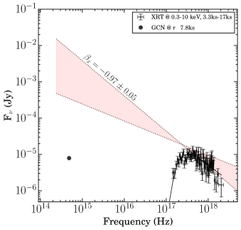
For GRB 201216C, similarly, we created a optical-X-ray SED from optical to X-ray frequencies and extrapolated our X-ray spectral index (@) to the lower frequency, see Figure 7, lower panel. The Galactic corrected r band magnitude lies much below the extrapolated X-ray power-law slope. Considering no spectral break and a spectral break between X-ray and optical frequencies in the SED, we estimated the intrinsic optical flux by extrapolating the X-ray spectral index at r-band frequency. By comparing the estimated optical flux to the observed VLT optical flux at 2.19 h Izzo et al. (2020), we determine the host extinction in the r-band mag, supporting the dark nature of the burst, consistent with the result of Rhodes et al. (2022).
4 Discussion
4.1 Bulk Lorentz factor and characteristic fireball radius of VHE detected GRBs
There are different ways to derive/put constraints on the bulk Lorentz factor of GRBs (Ghirlanda et al., 2018). In this section, we have derived the values of bulk Lorentz factor for VHE detected GRBs using three different methods using onset of the afterglow, using Liang correlation, and using prompt - relation.
Using onset of the afterglow: We have used equation 4 to calculate the bulk Lorentz factors for GRB 201015A, GRB 201216C, and the other four well-known VHE detected GRBs, GRB 160821B (this GRB has no firm detection, but an evidence of signal at VHE at the level of 3 ), GRB 180720B, GRB 190114C, and GRB 190829A. We noted that for the last four VHE GRBs, there is no early bump/peak observed in their optical afterglow light curves. For such cases, we assumed the earliest optical observations as upper limits for the peak time for the afterglow and constrained the lower limit on the bulk Lorentz factor for these bursts. The calculated values of using equation 4, and corresponding peak times are listed in the first column of Table 3, for both types of surrounding media. In addition, we also calculated the deceleration radius of the fireball at the peak time using the following equation taken from M2007:
| (5) |
The calculated values of deceleration radius are also listed in the first column of Table 3. Further, we also verified these parameters using various correlations between the bulk Lorentz factor and prompt emission properties, such as - , and - and noted the the values are consistent for the sub-sample of VHE detected GRBs (see Figure 16).
Using Liang correlation: Liang et al. 2010 (hereafter L2010) extensively searched for the onset of the afterglow in the X-ray and optical afterglow light curves using the published literature and Swift-XRT catalog. They found that twenty bursts in the optical and twelve bursts in the X-ray bands displayed the onset features in their corresponding afterglow light curves. In addition, L2010 also discovered tight correlations between the isotropic equivalent gamma-ray energy and the initial bulk Lorentz factor of the fireball. The correlation can be given as: .
For all the seven known VHE detected GRBs, we derive the bulk Lorentz factor using - correlation, and calculated values along with T90 are listed in the second column of Table 3. We also calculated the fireball radius at the end of the prompt emission using the following relation: R using t T90 in the equation. The calculated values of fireball radius given are also listed in the second column of Table 3.
Additionally, L2010 also studied the correlations between the characteristic bump/onset parameters, such as peak time, FWHM, isotropic gamma-ray energy, etc., and they found that most of these parameters are strongly correlated with each other. We also compare the properties of the observed bump in the early optical light curves of GRB 201015A and GRB 201216C with the known correlations. We noted that most of the characteristic parameters of the observed bump in the early optical light curves of GRB 201015A and GRB 201216C are consistent with the correlations studied by L2010, confirming the nature of the bumps due to the onset of forward shocks in the external ambient medium. However, GRB 201216C does not follow the correlation between and optical peak luminosity (), supporting the dark behavior of GRB 201216C (Rhodes et al., 2022). The correlations between the different parameters of the optical bumps of GRB 201015A and GRB 201216C, along with data taken from L2010 are shown in Figure 17 of the appendix.
Using Prompt - relation: In addition to the above methods, we also used the prompt - (minimum variability time scales) relation to calculate the lower bound on the bulk Lorentz factor () and to calculate emission radius during the prompt emission phase. We used the following relations between - and - derived by Golkhou et al. 2015 (hereafter G2015):
| (6) |
| (7) |
We calculated the minimum variability time scales for the VHE detected GRBs using the Bayesian block method on the prompt emission light curve in the energy range of 8-900 keV for Fermi-GBM and 15-350 keV for Swift-BAT, respectively. The Bayesian blocks utilize the statistically significant changes to bin the prompt emission light curves of these bursts. We determine the minimum bin size, and the minimal variability time scales are equal to half of the width of the smallest bin of Bayesian blocks (Vianello et al., 2018). The calculated values of , , and are listed in the third column of Table 3. We noted that the emission radius lies in the range of cm - cm for all the seven known VHE detected GRBs, consistent with the results of G2015. The calculated emission radius for these VHE detected GRBs is much larger than the typical emission radius of the photosphere, suggesting that the emission took place in an optically thin region away from the central engine (Caballero-García et al., 2022; Burgess et al., 2020).
4.2 Lorentz factor evolution and the possible jet composition
The evolution of the bulk Lorentz factor can provide insight into the jet composition, the prompt emission location, and the radiation physics of GRBs. The jet of GRBs can be matter dominated (originated due to photosphere) or Poynting flux dominated (originated due magnetic reconnection). However, a third hybrid jet composition (quasi-thermal component together with a non-thermal component) formed in the internal shocks, is possible. In such hybrid case, it is expected that the Lorentz factor remains almost constant during the prompt emission phase and decreases during the onset of afterglow (Lin et al., 2019). On the other hand, in the case of Poynting flux dominated jet (a part of the magnetic field energy dissipates to accelerate the GRB jet), the Lorentz factor measured during the onset of afterglow is expected to be larger than that measured during the prompt phase (Zhang & Zhang, 2014).
| VHE detected | M2007 | L2010 | G2015 | ||||||
|---|---|---|---|---|---|---|---|---|---|
| GRBs | (s) | (cm) | T90 (s) | (cm) | (s) | (cm) | |||
| 160821B | - | - | - | 0.5 | 69 8 | 1.181014 | 0.068 | 88.74 | 2.781013 |
| 180720B | 73 | 576 | 2.191017 | 49 | 506 66 | 4.551017 | 0.024 | 457.20 | 1.821014 |
| 190114C | 33.2 | 341 | 4.101016 | 25 | 407 41 | 1.741017 | 0.016 | 472.86 | 1.531014 |
| 190829A | - | - | - | 63 | 76 8 | 2.021016 | 0.210 | 47.74 | 2.671013 |
| 201015A | 184.64 | 204 | 8.161016 | 9.78 | 143 4 | 8.411015 | 92.07 | 4.811013 | |
| 201216C | 179.9 | 310 | 1.231017 | 29.9 | 513 68 | 2.241017 | 0.152 | 286.99 | 3.601014 |
| 221009A | 179 | 440 | 4.501017 | 327 | 757 | 9.71018 | 0.001 | 450.01 | 1.11013 |
In § 4.1, we have calculated the bulk Lorentz factor of the fireball for GRB 201015A and GRB 201216C at different epochs to examine the evolution of Lorentz factor and constrain the possible jet composition. Initially, we calculated the the bulk Lorentz factor values during the prompt emission phase using two different methods: the first one using the relation between the lower limit on bulk Lorentz factor and the minimum variability time scale (G2015). In the second method, we have used the tight correlation between the and total isotropic gamma-ray energy released during the prompt emission to calculate the bulk Lorentz factor (L2010). Finally, we calculated the bulk Lorentz factor values (for the different types of ambient medium) during the onset of forward shock emission using the observed early peak in the optical afterglow light curves (Sari & Piran, 1999; Molinari et al., 2007; Ghirlanda et al., 2018).
In the case of GRB 201015A, the measured values of at different epochs are following: 92.07 using G2015, 143 using L2010, and 204 for ISM-like medium using the onset of forward shock emission. The lower limit on the measured value of (using G2015) is consistent with that measured using the tight correlation between and . For GRB 201015A, the closure relations support a homogeneous medium (see § 3.2.3), also consistent with Giarratana et al. (2022). The value of the bulk Lorentz factor during the onset of the afterglow increases for an ISM-like ambient medium, support a Poynting flux dominated jet composition for GRB 201015A, although there is not a very large difference between the bulk Lorentz factor values at different epochs. In the case of GRB 201216C, the measured values of at different epochs are following: 286 using G2015, 513 using L2010, and 310 for wind-like medium using the onset of forward shock emission. For this GRB also, the lower limit on the (using G2015) is lower than that measured using tight correlation between the and . For GRB 201216C, the closure relations support a wind-like medium (see § 3.2.3), also consistent with Rhodes et al. (2022). The value of the bulk Lorentz factor during the onset of the afterglow decreases for a wind-like ambient medium, support a matter dominated jet composition for GRB 201216C.
4.3 Progenitors of GRB 201015A and GRB 201216C: Collapsar origin?
The recent discoveries of short GRBs (GRB 200826A, GRB 211227A) from the collapse of massive stars (Ahumada et al., 2021; Lü et al., 2022) and long GRB (GRB 211211A) from binary mergers (Rastinejad et al., 2022) challenge our understanding about progenitor systems of GRBs. In this section, we examine the possible progenitors of GRB 201015A and GRB 201216C. There are two possible models (collapsar and binary merger) for the progenitor of GRBs. According to the Collapsar model, the central engine (black hole or magnetar) forms after the death of a massive stellar object emits a jet that successfully penetrates the preexisting envelope around the progenitor star. If the jet does not have sufficient energy to breakout, it deposits all of its energy into the surrounding envelope to form a mildly relativistic cocoon around it. This process is known as shock breakout and it gives emission in gamma-rays, with a luminosity 2-3 orders less than typical long GRBs (Bromberg et al., 2011). Such subclass of GRBs with low isotropic gamma-ray luminosity (order of erg ) emitted during the prompt emission phase is assumed to have a different origin than normal long GRBs. In the VHE detected GRBs sample, GRB 190829A is a peculiar low-luminosity GRB with no shock breakout origin Chand et al. (2020). In addition, GRB 201015A also belongs to the low-luminosity family of GRBs with a supernova bump in the late optical light curve, which motivate us to test whether it has a collapsar or shock breakout origin.
In the case of collapsar origin, it is expected that the observed duration (T90) of the burst should be greater than the jet breakout time () from the surrounding envelope. Bromberg et al. (2011) suggested that if the ratio T90/ 1 and the jet failed to cross the envelope, in such case, the burst is expected to originate from the shock breakout. On the other hand, if T90/ 1 and the jet successfully crosses the envelope, the burst is expected to originate from the collapsar. We calculated the jet breakout time for GRB 201015A the following equation given by Bromberg et al. (2011): .
The jet breakout time depends on the isotropic equivalent luminosity, the observed opening angle, progenitor mass, and radiation efficiency. To calculate Tbreak for GRB 201015A, we assume the typical values of M = 15, = and (Bromberg et al., 2011). We obtained the ratio T90/ = 1.75 for GRB 201015A, which supports the collapsar origin of the burst. We also calculated the T90/Tbreak ratio for GRB 201216C considering = and with progenitor mass 12 and 25 (Rhodes et al., 2022) and found that T90/ lies in the range of 30–163, which confirms the collapsar origin of GRB 201216C.
4.4 Comparison of GRB 201015A and GRB 201216C with other VHE detected GRBs
In all the seven cases of VHE GRBs, VHE photons were detected during the afterglow phase, although, VHE photons may enrich the prompt emission of GRBs also. In the present section, we compared the afterglow results obtained for GRB 201015A and GRB 201216C (see § 3) with a sample of well-known VHE detected GRBs (MAGIC Collaboration et al., 2019a, b; Nava, 2021; Noda & Parsons, 2022; Fraija et al., 2019b). In addition to afterglow comparison, we also collected the prompt emission properties of VHE detected GRBs, listed in Table 1.
4.4.1 Comparison of X-ray and optical afterglow light curves of VHE detected GRBs
In the present section, we compared the X-ray and the optical (see Figure 14 of the appendix) afterglow luminosity light curves of GRB 201015A and GRB 201216C with other well-studied VHE detected GRBs (GRB 160821B, GRB 180720B, GRB 190114C, GRB 190829A, and GRB 221009A). In addition, we also included X-ray (if available) and optical (if available) light curves of a nearly complete sample of nearby and supernovae-connected GRBs (GRB 050525A/SN 2005nc ( = 0.606), GRB 081007A/SN 2008hw ( = 0.530), GRB 091127A/SN 2009nz ( = 0.490), GRB 101219B/SN 2010ma ( = 0.552), GRB 111209A/SN 2011kl ( = 0.677), GRB 130702A/SN 2013dx ( = 0.145), GRB 130831A/SN 2013fu ( = 0.479), GRB 060218/SN 2006aj ( = 0.033), GRB 120422A/SN 2012bz ( = 0.282), GRB 130427A/SN ( = 0.340), GRB 190114C/SN ( = 0.425), GRB 190829A/SN 2019oyw ( = 0.078), GRB 200826A/SN ( = 0.748)) for the comparison as most of VHE detected bursts are nearby and connected with supernovae. The comparison of X-ray afterglow light curves indicates that VHE detected GRB 180720B and GRB 201216C have extremely bright X-ray emission (just below the brightest X-ray emission observed from GRB 130427A at early epochs). GRB 221009A and GRB 190114C also have a very bright X-ray emission but less than those of GRB 180720B and GRB 201216C at early epochs. On the other hand, GRB 160821B, GRB 190829A, and GRB 201015A have a faint X-ray emission. The X-ray afterglow of GRB 201015A has a nearly comparable brightness with GRB 190829A. GRB 160821B, being a short burst, has the faintest X-ray light curve (after the steep decay phase) with respect to present VHE sample.
For the optical afterglow light curve comparison, we collected the R band light curve of VHE detected GRBs (other than GRB 221009A) from the literature (MAGIC Collaboration et al., 2019a; Misra et al., 2021; Gupta et al., 2021a; Fraija et al., 2019b; Jordana-Mitjans et al., 2020). For GRB 221009A, we collected the optical data from the GCN circulars121212https://gcn.gsfc.nasa.gov/other/221009A.gcn3. For a nearly complete sample of nearby and supernovae-connected GRBs, we obtained the optical data from Kumar et al. (2022a) and references therein. We noted that GRB 180720B has the highest optical luminosity at early epochs in comparison to the present sample (similar to the X-ray light curve) and the light curve displays a smooth power-law decay across the emission period (Fraija et al., 2019b). At later phases ( 0.2 days post burst), GRB 221009A seems to have the highest optical luminosity in comparison to the present sample. In the case of GRB 201216C, despite of the very bright X-ray emission, the optical light curve is one of the faintest with respect to present sample, typical to those observed in the case of dark GRBs. Further, we noted that GRB 201015A and GRB 201216C have a comparable optical luminous light curves. GRB 190114C (Gupta et al., 2021a), GRB 190829A (Hu et al., 2021), and GRB 201015A (Giarratana et al., 2022) had a late time bump in their optical light curve associated with their underlying supernovae explosions. In addition, we noted that GRB 201015A and GRB 201216C are the only the bursts with very early smooth bump (the onset of the forward shock) in their optical light curves with respect to present sample.
4.4.2 Possible origin of VHE emission from high and low luminosity bursts
The broadband afterglow observations of the VHE detected GRBs could not be explained by the typical external shock synchrotron model (MAGIC Collaboration et al., 2019b; H.E.S.S. Collaboration et al., 2021). The multi-wavelength modeling of the observed double bump SEDs of VHE detected GRBs demands an additional SSC/Inverse Compton component. VHE detected GRBs are expected to be luminous and nearby such as GRB 180720B, GRB 190114C, and GRB 221009A. However, some of the recent detection of VHE emission from low/intermediate-luminosity bursts (such as GRB 190829A, and GRB 201015A), open a new question about their possible progenitors and viewing geometry. The high luminosity GRBs are typically observed on-axis with narrow viewing, on the other hand, low-luminosity bursts are typically observed off-axis with wide viewing angle. Recently, some authors (Sato et al., 2022; Rhodes et al., 2022) used two different jet components (narrow and wide) model to explain the origin of the observed properties of high and low luminosity VHE detected GRBs. According to this model, the early broadband emission of the high luminosity GRBs are explained using narrow jet component with typical opening angle . On the other hand, the low luminosity GRBs are explained using wide jet component with typical opening angle (Sato et al., 2022). Sato et al. (2022) performed the broadband modeling of nearby and low-luminosity GRB 190829A using two-component jet model and noted that the prompt and afterglow emissions could not be described from the narrow jet component. The observed low/intermediate luminosity nature of GRB 190829A is explained by assuming that the viewing angle is greater than the opening angle of its narrow jet component (off-axis observations). GRB 201015A is also a nearby intermediate luminosity GRB and might have a very similar viewing geometry to GRB 190829A (viewing angle greater than the narrow jet opening angle). In the case of GRB 180720B, and GRB 190114C, the observed high luminosity nature of these GRBs are explained from emission within the narrow jet component (on-axis observations). The same applies to GRB 201216C, given its observed high luminosity.
The observed typical sub-TeV bump are explained either using SSC or external Inverse Compton (MAGIC Collaboration et al., 2019b; Abdalla et al., 2019). According to two component model, during the early phase, both the components (narrow and wide) of the jet have almost equal velocities. This negligible difference in the velocities helps to discard the possibility of the contribution from the external Inverse Compton during early phase (Sato et al., 2022). Therefore, the SSC emission mechanism is expected to explain the early VHE emission, for example GRB 190114C, and GRB 190829A MAGIC Collaboration et al. (2019b); H.E.S.S. Collaboration et al. (2021). In the case of GRB 180720B, VHE photons were observed several hours after the detection. Therefore, considering the two jets moving at different velocities, Inverse Compton significantly contributed to the observed VHE emission (Abdalla et al., 2019). In the case of GRB 201216C, considering the synchrotron process as a possible radiation mechanism at t 3 - s post burst at X-ray frequencies, we extrapolated the X-ray spectral index towards the GeV-TeV energies (for the spectral regime ), and estimated the expected flux density Jy, and Jy at 1 GeV and 0.1 TeV, respectively. Fermi-LAT could not detect the GeV emission from GRB 201216C during the interval T0 + 3500 s to T0 + 5500 s post burst. This is in agreement with the fact that the expected flux density at 1 GeV at t 3 - s post burst is below the sensitivity of Fermi-LAT instrument. Furthermore, from the observed peak in the early optical light curve of GRB 201216C, we calculated the initial Lorentz factor of the burst 300. With this Lorentz factor and , photons of maximum energy, 15 GeV, are allowed by synchrotron process Fraija et al. (2019b).
Similarly, for GRB 201015A expected flux density Jy, and Jy at 1 GeV and 0.1 TeV, respectively, is obtained at 3ks-5ks. A bulk Lorentz factor 200 is obtained from the observed peak in the optical light curve. With this Lorentz factor and , we estimated the maximum energy of synchrotron photons 14 GeV Fraija et al. (2019b).
Therefore, observed early VHE emission could not be explained using the synchrotron emission model. The previous discussion suggests that the early detection of VHE photons from GRB 201015A and GRB 201216C required that the ultra-relativistic outflow boosts the energy of low-energy synchrotron photons to the VHE energies via the SSC process.
5 Summary and Conclusion
In this work, we presented a detailed analysis of the prompt and afterglow emission of two VHE detected GRBs GRB 201015A and GRB 201216C and their comparison with a subset of similar bursts. In spite of showing prompt emission characteristics of other typical LGRBs, GRB 201015A is a low/intermediate luminosity whereas GRB 201216C is one of the high luminosity ones. Detailed time-resolved spectral analysis of Fermi observations of GRB 201216C suggests that the low energy spectral index () remained within the expected values of synchrotron slow and fast cooling limits supporting the synchrotron emission as a possible emission mechanism. Searches for the additional thermal component indicate that some of the Bayesian bins have a quasi-thermal component centered around the beginning or near the peaks of the light curve.
Further, we studied the evolution of spectral parameters and find a rare feature where and both showing flux tracking behavior (double tracking) throughout the duration of GRB 201216C as published recently (Gupta et al., 2021b), proposing the observed relation between and flux in terms of fireball cooling and expansion. In such a scenario, during the fireball expansion, the magnetic field reduces resulting in a lower intensity and . However, increased central engine activity during the bursting phase might increase the magnetic field, resulting in higher and/or intensity. If such a scenario is true, the magnetic field should be strongly correlated with (Gao et al., 2021). Interestingly, we found a strong correlation between (derived using empirical Band function) and the magnetic field (B) (derived using the physical Synchrotron model), supporting our results discussed above. On the other hand, strong correlation observed between -flux can be explained in terms of sub-photospheric heating in a flow of varying entropy (Ryde et al., 2019).
Our earliest optical observations of the afterglow of GRB 201015A using FRAM-ORM and BOOTES and GRB 201216C using FRAM-ORM robotic telescopes display a smooth bumps, consistent with the onset of afterglow in the framework of the external forward shock model (Sari & Piran, 1999). Using the observed optical peak, we determined the initial bulk Lorentz factors of GRB 201015A and GRB 201216C: = 204 for the ISM-like, and = 310 for wind-like ambient media, respectively. Further, we studied evolution of the Lorentz factors and constrain the possible jet compositions for both the bursts. Evolution of the Lorentz factors suggests a Poynting flux-dominated jet for GRB 201015A whereas for GRB 201216C, preference for an internal shock-dominated jet, consistent with time-resolved spectral analysis. Furthermore, we investigated the possible progenitors of GRB 201015A and GRB 201216C by constraining the time taken by the jet to break through the surrounding envelope () using the relation given by Bromberg et al. (2011), and taking the ratio of observed T90 to . We find that for both the bursts, this ratio is greater than one, supporting the collapsar as the possible progenitors of GRB 201015A and GRB 201216C. Also, late time optical follow-up observations of GRB 201015A reveal an associated supernova (Giarratana et al., 2022), additional evidence confirming the collapsar origin.
Finally, we compare the properties of GRB 201015A and GRB 201216C with other similar VHE detected GRBs. Our findings suggest that VHE emission is common both in high and low luminosity GRBs. Our study also suggests that SSC process is needed to explain the VHE emission of these bursts. Early follow-up observations of similar sources using robotic telescopes are very crucial not only to constrain the Lorentz factors/their evolution but also to decipher other yet least explored aspects of underlying physics like radiation mechanism, jet compositions, etc.
Acknowledgments
Authors are thankful to the anonymous referee for his/her positive and valuable comments. RG and SBP acknowledge the financial support of ISRO under AstroSat archival Data utilization program (DS2B-13013(2)/1/2021-Sec.2). AA acknowledges funds and assistance provided by the Council of Scientific & Industrial Research (CSIR), India with file no. 09/948(0003)/2020-EMR-I. AJCT acknowledges support from the Spanish Ministry project PID2020-118491GB-I00 and Junta de Andalucia grant P20_010168. YDH acknowledges support under the additional funding from the RYC2019-026465-I. MCG acknowledges support from the Ramón y Cajal Fellowship RYC2019-026465-I (funded by the MCIN/AEI /10.13039/501100011033 and the European Social Funding). This research has used data obtained through the HEASARC Online Service, provided by the NASA-GSFC, in support of NASA High Energy Astrophysics Programs. SBP thankfully acknowledge inclusion of the photometric calibration data of GRB 201015A taken with the 4Kx4K CCD Imager acquired as a part of the present analysis and extends sincere thanks to all the observing and support staff of the 3.6m DOT to maintain and run the observational facilities at Devasthal Nainital.
References
- Abbott et al. (2017) Abbott, B. P., Abbott, R., Abbott, T. D., et al. 2017, The Astrophysical Journal, 848, L13, doi: 10.3847/2041-8213/aa920c
- Abdalla et al. (2019) Abdalla, H., Adam, R., Aharonian, F., et al. 2019, Nature, 575, 464, doi: 10.1038/s41586-019-1743-9
- Ahumada et al. (2021) Ahumada, T., Singer, L. P., Anand, S., et al. 2021, Discovery and confirmation of the shortest gamma ray burst from a collapsar. https://arxiv.org/abs/2105.05067
- Amati (2006) Amati, L. 2006, Monthly Notices of the Royal Astronomical Society, 372, 233, doi: 10.1111/j.1365-2966.2006.10840.x
- Arnaud (1996) Arnaud, K. A. 1996, in Astronomical Society of the Pacific Conference Series, Vol. 101, Astronomical Data Analysis Software and Systems V, ed. G. H. Jacoby & J. Barnes, 17
- Astropy Collaboration et al. (2013) Astropy Collaboration, Robitaille, T. P., Tollerud, E. J., et al. 2013, A&A, 558, A33, doi: 10.1051/0004-6361/201322068
- Band et al. (1993) Band, D., Matteson, J., Ford, L., et al. 1993, ApJ, 413, 281, doi: 10.1086/172995
- Barthelmy et al. (2005) Barthelmy, S. D., Barbier, L. M., Cummings, J. R., et al. 2005, Space Sci. Rev., 120, 143, doi: 10.1007/s11214-005-5096-3
- Beardmore et al. (2020) Beardmore, A. P., Gropp, J. D., Kennea, J. A., et al. 2020, GRB Coordinates Network, 29061, 1
- Becker (2015) Becker, A. 2015, HOTPANTS: High Order Transform of PSF ANd Template Subtraction, Astrophysics Source Code Library, record ascl:1504.004. http://ascl.net/1504.004
- Bissaldi et al. (2020) Bissaldi, E., Omodei, N., Kocevski, D., et al. 2020, GRB Coordinates Network, 29076, 1
- Blandford & McKee (1976) Blandford, R. D., & McKee, C. F. 1976, Physics of Fluids, 19, 1130, doi: 10.1063/1.861619
- Bromberg et al. (2011) Bromberg, O., Nakar, E., & Piran, T. 2011, ApJ, 739, L55, doi: 10.1088/2041-8205/739/2/L55
- Burgess (2014) Burgess, J. M. 2014, MNRAS, 445, 2589, doi: 10.1093/mnras/stu1925
- Burgess et al. (2020) Burgess, J. M., Bégué, D., Greiner, J., et al. 2020, Nature Astronomy, 4, 174, doi: 10.1038/s41550-019-0911-z
- Burrows et al. (2005) Burrows, D. N., Hill, J. E., Nousek, J. A., et al. 2005, Space Sci. Rev., 120, 165, doi: 10.1007/s11214-005-5097-2
- Caballero-García et al. (2022) Caballero-García, M. D., Gupta, R., Pandey, S. B., et al. 2022, arXiv e-prints, arXiv:2205.07790. https://arxiv.org/abs/2205.07790
- Campana et al. (2020) Campana, S., Cusumano, G., Evans, P. A., et al. 2020, GRB Coordinates Network, 29064, 1
- Chand et al. (2020) Chand, V., Banerjee, A., Gupta, R., et al. 2020, ApJ, 898, 42, doi: 10.3847/1538-4357/ab9606
- de Ugarte Postigo et al. (2020a) de Ugarte Postigo, A., Kann, D. A., Blazek, M., et al. 2020a, GRB Coordinates Network, 28649, 1
- de Ugarte Postigo et al. (2020b) de Ugarte Postigo, A., Thöne, C. C., Martín, S., et al. 2020b, A&A, 633, A68, doi: 10.1051/0004-6361/201936668
- de Ugarte Postigo et al. (2022) de Ugarte Postigo, A., et al. 2022, GRB Coordinates Network. https://gcn.gsfc.nasa.gov/gcn3/32648.gcn3
- D’Elia et al. (2020) D’Elia, V., Ambrosi, E., Barthelmy, S. D., et al. 2020, GRB Coordinates Network, 28632, 1
- Dichiara et al. (2022) Dichiara, S., Gropp, J. D., Kennea, J. A., et al. 2022, GRB Coordinates Network. https://gcn.gsfc.nasa.gov/gcn3/32632.gcn3
- Evans et al. (2007) Evans, P. A., Beardmore, A. P., Page, K. L., et al. 2007, A&A, 469, 379, doi: 10.1051/0004-6361:20077530
- Evans et al. (2009) —. 2009, MNRAS, 397, 1177, doi: 10.1111/j.1365-2966.2009.14913.x
- Fong et al. (2015) Fong, W., Berger, E., Margutti, R., & Zauderer, B. A. 2015, ApJ, 815, 102, doi: 10.1088/0004-637X/815/2/102
- Fraija et al. (2019a) Fraija, N., Dichiara, S., Pedreira, A. C. C. d. E. S., et al. 2019a, ApJ, 879, L26, doi: 10.3847/2041-8213/ab2ae4
- Fraija et al. (2021) Fraija, N., Veres, P., Beniamini, P., et al. 2021, ApJ, 918, 12, doi: 10.3847/1538-4357/ac0aed
- Fraija et al. (2019b) Fraija, N., Dichiara, S., Pedreira, A. C. C. d. E. S., et al. 2019b, ApJ, 885, 29, doi: 10.3847/1538-4357/ab3e4b
- Frederiks et al. (2020) Frederiks, D., Golenetskii, S., Aptekar, R., et al. 2020, GRB Coordinates Network, 29084, 1
- Fukami et al. (2022) Fukami, S., Berti, A., Loporchio, S., et al. 2022, in 37th International Cosmic Ray Conference, 788, doi: 10.22323/1.395.0788
- Gao et al. (2015) Gao, H., Wang, X.-G., Mészáros, P., & Zhang, B. 2015, ApJ, 810, 160, doi: 10.1088/0004-637X/810/2/160
- Gao et al. (2021) Gao, H.-X., Geng, J.-J., & Huang, Y.-F. 2021, A&A, 656, A134, doi: 10.1051/0004-6361/202141647
- Ghirlanda et al. (2018) Ghirlanda, G., Nappo, F., Ghisellini, G., et al. 2018, A&A, 609, A112, doi: 10.1051/0004-6361/201731598
- Giarratana et al. (2022) Giarratana, S., Rhodes, L., Marcote, B., et al. 2022, arXiv e-prints, arXiv:2205.12750. https://arxiv.org/abs/2205.12750
- Goldstein et al. (2017) Goldstein, A., Veres, P., Burns, E., et al. 2017, The Astrophysical Journal, 848, L14, doi: 10.3847/2041-8213/aa8f41
- Golenetskii et al. (1983) Golenetskii, S. V., Mazets, E. P., Aptekar, R. L., & Ilinskii, V. N. 1983, Nature, 306, 451, doi: 10.1038/306451a0
- Golkhou et al. (2015) Golkhou, V. Z., Butler, N. R., & Littlejohns, O. M. 2015, ApJ, 811, 93, doi: 10.1088/0004-637X/811/2/93
- Gupta et al. (2021a) Gupta, R., Pandey, S. B., Castro-Tirado, A. J., et al. 2021a, in Revista Mexicana de Astronomia y Astrofisica Conference Series, Vol. 53, Revista Mexicana de Astronomia y Astrofisica Conference Series, 113–123, doi: 10.22201/ia.14052059p.2021.53.23
- Gupta et al. (2021b) Gupta, R., Oates, S. R., Pandey, S. B., et al. 2021b, MNRAS, 505, 4086, doi: 10.1093/mnras/stab1573
- Gupta et al. (2022a) Gupta, R., Bhushan Pandey, S., Kumar, A., et al. 2022a, arXiv e-prints, arXiv:2205.13940. https://arxiv.org/abs/2205.13940
- Gupta et al. (2022b) Gupta, R., Gupta, S., Chattopadhyay, T., et al. 2022b, MNRAS, 511, 1694, doi: 10.1093/mnras/stac015
- Gupta et al. (2022c) Gupta, R., Kumar, A., Pandey, S. B., et al. 2022c, Journal of Astrophysics and Astronomy, 43, 11, doi: 10.1007/s12036-021-09794-4
- H.E.S.S. Collaboration et al. (2021) H.E.S.S. Collaboration, Abdalla, H., Aharonian, F., et al. 2021, Science, 372, 1081, doi: 10.1126/science.abe8560
- Hjorth et al. (2003) Hjorth, J., Sollerman, J., Møller, P., et al. 2003, Nature, 423, 847, doi: 10.1038/nature01750
- Hu et al. (2020) Hu, Y. D., Fernandez-Garcia, E., Castro-Tirado, A. J., et al. 2020, GRB Coordinates Network, 28645, 1
- Hu et al. (2021) Hu, Y. D., Castro-Tirado, A. J., Kumar, A., et al. 2021, A&A, 646, A50, doi: 10.1051/0004-6361/202039349
- Huang et al. (2020) Huang, X.-L., Liang, E.-W., Liu, R.-Y., Cheng, J.-G., & Wang, X.-Y. 2020, ApJ, 903, L26, doi: 10.3847/2041-8213/abc330
- Huang et al. (2022) Huang, Y., Hu, S., Chen, S., et al. 2022, GRB Coordinates Network. https://gcn.gsfc.nasa.gov/gcn3/32677.gcn3
- Hunter (2007) Hunter, J. D. 2007, Computing in Science and Engineering, 9, 90, doi: 10.1109/MCSE.2007.55
- Izzo et al. (2020) Izzo, L., Malesani, D. B., & Kann, D. A. 2020, GRB Coordinates Network, 29066, 1
- Jelinek et al. (2020a) Jelinek, M., Strobl, J., Karpov, S., et al. 2020a, GRB Coordinates Network, 28664, 1
- Jelinek et al. (2020b) —. 2020b, GRB Coordinates Network, 29070, 1
- Jordana-Mitjans et al. (2020) Jordana-Mitjans, N., Mundell, C. G., Kobayashi, S., et al. 2020, ApJ, 892, 97, doi: 10.3847/1538-4357/ab7248
- Kargatis et al. (1994) Kargatis, V. E., Liang, E. P., Hurley, K. C., et al. 1994, ApJ, 422, 260, doi: 10.1086/173724
- Kennea et al. (2020) Kennea, J. A., Tagliaferri, G., Campana, S., et al. 2020, GRB Coordinates Network, 28635, 1
- Kobayashi & Zhang (2003) Kobayashi, S., & Zhang, B. 2003, ApJ, 582, L75, doi: 10.1086/367691
- Kouveliotou et al. (1993) Kouveliotou, C., Meegan, C. A., Fishman, G. J., et al. 1993, ApJ, 413, L101, doi: 10.1086/186969
- Kumar et al. (2022a) Kumar, A., Pandey, S. B., Gupta, R., et al. 2022a, New A, 97, 101889, doi: 10.1016/j.newast.2022.101889
- Kumar et al. (2022b) Kumar, A., Pandey, S. B., Singh, A., et al. 2022b, Journal of Astrophysics and Astronomy, 43, 27, doi: 10.1007/s12036-022-09798-8
- Kumar & Zhang (2015) Kumar, P., & Zhang, B. 2015, Physics Reports, 561, 1–109, doi: 10.1016/j.physrep.2014.09.008
- Lamb et al. (2019) Lamb, G. P., Tanvir, N. R., Levan, A. J., et al. 2019, ApJ, 883, 48, doi: 10.3847/1538-4357/ab38bb
- Li et al. (2019) Li, L., Geng, J.-J., Meng, Y.-Z., et al. 2019, ApJ, 884, 109, doi: 10.3847/1538-4357/ab40b9
- Liang et al. (2010) Liang, E.-W., Yi, S.-X., Zhang, J., et al. 2010, ApJ, 725, 2209, doi: 10.1088/0004-637X/725/2/2209
- Lin et al. (2019) Lin, D.-B., Lu, R.-J., Du, S.-S., et al. 2019, ApJ, 883, 187, doi: 10.3847/1538-4357/ab3a56
- Lipunov et al. (2020) Lipunov, V., Gorbovskoy, E., Kornilov, V., et al. 2020, GRB Coordinates Network, 28633, 1
- Lü et al. (2022) Lü, H.-J., Yuan, H.-Y., Yi, T.-F., et al. 2022, ApJ, 931, L23, doi: 10.3847/2041-8213/ac6e3a
- Lü et al. (2012) Lü, J., Zou, Y.-C., Lei, W.-H., et al. 2012, ApJ, 751, 49, doi: 10.1088/0004-637X/751/1/49
- MAGIC Collaboration et al. (2019a) MAGIC Collaboration, Acciari, V. A., Ansoldi, S., et al. 2019a, Nature, 575, 455, doi: 10.1038/s41586-019-1750-x
- MAGIC Collaboration et al. (2019b) —. 2019b, Nature, 575, 459, doi: 10.1038/s41586-019-1754-6
- Malacaria et al. (2020) Malacaria, C., Veres, P., Meegan, C., Bissaldi, E., & Fermi GBM Team. 2020, GRB Coordinates Network, 29073, 1
- Malesani et al. (2020) Malesani, D. B., de Ugarte Postigo, A., & Pursimo, T. 2020, GRB Coordinates Network, 28637, 1
- Markwardt et al. (2020) Markwardt, C. B., Barthelmy, S. D., Cummings, J. R., et al. 2020, GRB Coordinates Network, 28658, 1
- Meegan et al. (2009) Meegan, C., Lichti, G., Bhat, P., et al. 2009, The Astrophysical Journal, 702, 791, doi: 10.1088/0004-637X/702/1/791
- Minaev & Pozanenko (2020) Minaev, P. Y., & Pozanenko, A. S. 2020, MNRAS, 492, 1919, doi: 10.1093/mnras/stz3611
- Misra et al. (2021) Misra, K., Resmi, L., Kann, D. A., et al. 2021, MNRAS, 504, 5685, doi: 10.1093/mnras/stab1050
- Molinari et al. (2007) Molinari, E., Vergani, S. D., Malesani, D., et al. 2007, A&A, 469, L13, doi: 10.1051/0004-6361:20077388
- Nadella et al. (2020) Nadella, D., Waratkar, G., Vibhute, A., et al. 2020, GRB Coordinates Network, 29074, 1
- Nava (2021) Nava, L. 2021, Universe, 7, 503, doi: 10.3390/universe7120503
- Nava et al. (2012) Nava, L., Salvaterra, R., Ghirlanda, G., et al. 2012, MNRAS, 421, 1256, doi: 10.1111/j.1365-2966.2011.20394.x
- Noda & Parsons (2022) Noda, K., & Parsons, R. D. 2022, Galaxies, 10, 7, doi: 10.3390/galaxies10010007
- Norris et al. (1986) Norris, J. P., Share, G. H., Messina, D. C., et al. 1986, ApJ, 301, 213, doi: 10.1086/163889
- Oganesyan et al. (2019) Oganesyan, G., Nava, L., Ghirlanda, G., Melandri, A., & Celotti, A. 2019, Astronomy and Astrophysics, 628, A59, doi: 10.1051/0004-6361/201935766
- Pe’er (2015) Pe’er, A. 2015, Advances in Astronomy, 2015, 907321, doi: 10.1155/2015/907321
- Perna & Belczynski (2002) Perna, R., & Belczynski, K. 2002, The Astrophysical Journal, 570, 252, doi: 10.1086/339571
- Preece et al. (2000) Preece, R. D., Briggs, M. S., Mallozzi, R. S., et al. 2000, ApJS, 126, 19, doi: 10.1086/313289
- Rastinejad et al. (2022) Rastinejad, J. C., Gompertz, B. P., Levan, A. J., et al. 2022, arXiv e-prints, arXiv:2204.10864. https://arxiv.org/abs/2204.10864
- Ren et al. (2022) Ren, J., Wang, Y., & Zhang, L.-L. 2022, arXiv e-prints, arXiv:2210.10673. https://arxiv.org/abs/2210.10673
- Rhodes et al. (2022) Rhodes, L., van der Horst, A. J., Fender, R., et al. 2022, MNRAS, 513, 1895, doi: 10.1093/mnras/stac1057
- Ryde et al. (2019) Ryde, F., Yu, H.-F., Dereli-Bégué, H., et al. 2019, MNRAS, 484, 1912, doi: 10.1093/mnras/stz083
- Sari & Piran (1999) Sari, R., & Piran, T. 1999, ApJ, 520, 641, doi: 10.1086/307508
- Sari et al. (1998) Sari, R., Piran, T., & Narayan, R. 1998, The Astrophysical Journal, 497, L17–L20, doi: 10.1086/311269
- Sato et al. (2022) Sato, Y., Obayashi, K., Theodre Zhang, B., et al. 2022, arXiv e-prints, arXiv:2208.13987. https://arxiv.org/abs/2208.13987
- Scargle et al. (2013) Scargle, J. D., Norris, J. P., Jackson, B., & Chiang, J. 2013, The Astrophysical Journal, 764, 167, doi: 10.1088/0004-637x/764/2/167
- Shemi & Piran (1990) Shemi, A., & Piran, T. 1990, ApJ, 365, L55, doi: 10.1086/185887
- Stetson (1987) Stetson, P. B. 1987, PASP, 99, 191, doi: 10.1086/131977
- Suda et al. (2022) Suda, Y., Artero, M., Asano, K., et al. 2022, in 37th International Cosmic Ray Conference. 12-23 July 2021. Berlin, 797
- Tody (1986) Tody, D. 1986, in Society of Photo-Optical Instrumentation Engineers (SPIE) Conference Series, Vol. 627, Instrumentation in astronomy VI, ed. D. L. Crawford, 733, doi: 10.1117/12.968154
- Tody (1993) Tody, D. 1993, in Astronomical Society of the Pacific Conference Series, Vol. 52, Astronomical Data Analysis Software and Systems II, ed. R. J. Hanisch, R. J. V. Brissenden, & J. Barnes, 173
- Troja et al. (2019) Troja, E., Castro-Tirado, A. J., Becerra González, J., et al. 2019, MNRAS, 489, 2104, doi: 10.1093/mnras/stz2255
- Troja et al. (2022) Troja, E., Fryer, C. L., O’Connor, B., et al. 2022, arXiv e-prints, arXiv:2209.03363. https://arxiv.org/abs/2209.03363
- Ukwatta et al. (2020) Ukwatta, T. N., Barthelmy, S. D., Beardmore, A. P., et al. 2020, GRB Coordinates Network, 29080, 1
- Vianello (2018) Vianello, G. 2018, ApJS, 236, 17, doi: 10.3847/1538-4365/aab780
- Vianello et al. (2018) Vianello, G., Gill, R., Granot, J., et al. 2018, ApJ, 864, 163, doi: 10.3847/1538-4357/aad6ea
- Vianello et al. (2015) Vianello, G., Lauer, R. J., Younk, P., et al. 2015, arXiv e-prints, arXiv:1507.08343. https://arxiv.org/abs/1507.08343
- Vielfaure et al. (2020) Vielfaure, J. B., Izzo, L., Xu, D., et al. 2020, GRB Coordinates Network, 29077, 1
- Vinko & Wheeler (2022) Vinko, J., & Wheeler, J. C. 2022, The Astronomer’s Telegram, 15712, 1
- Willingale et al. (2013) Willingale, R., Starling, R. L. C., Beardmore, A. P., Tanvir, N. R., & O’Brien, P. T. 2013, MNRAS, 431, 394, doi: 10.1093/mnras/stt175
- Woosley (1993) Woosley, S. E. 1993, ApJ, 405, 273, doi: 10.1086/172359
- Yonetoku et al. (2004) Yonetoku, D., Murakami, T., Nakamura, T., et al. 2004, The Astrophysical Journal, 609, 935, doi: 10.1086/421285
- Zhang & Zhang (2014) Zhang, B., & Zhang, B. 2014, ApJ, 782, 92, doi: 10.1088/0004-637X/782/2/92
- Zhang et al. (2018) Zhang, B. B., Zhang, B., Castro-Tirado, A. J., et al. 2018, Nature Astronomy, 2, 69, doi: 10.1038/s41550-017-0309-8
- Zhang et al. (2021) Zhang, L.-L., Ren, J., Huang, X.-L., et al. 2021, ApJ, 917, 95, doi: 10.3847/1538-4357/ac0c7f
- Zhang et al. (2020) Zhang, Z. B., Jiang, M., Zhang, Y., et al. 2020, ApJ, 902, 40, doi: 10.3847/1538-4357/abb400
Appendix A Additional Figures
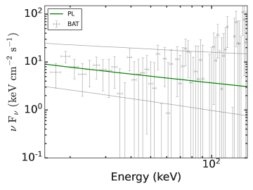
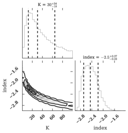
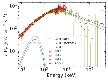
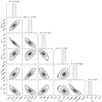
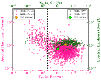
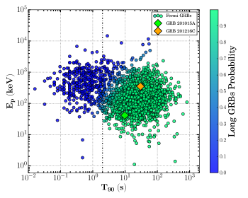
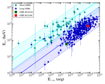
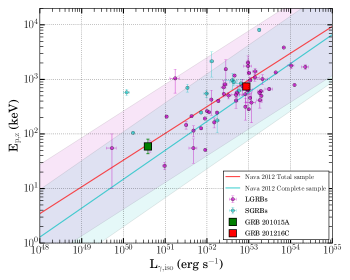
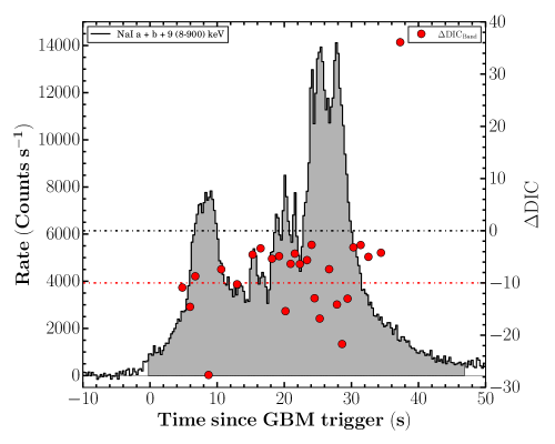
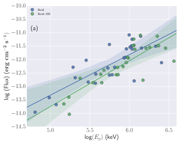
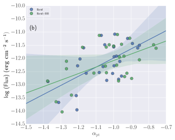
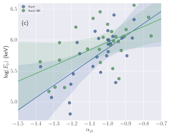
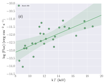
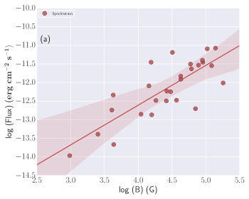
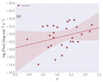
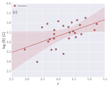
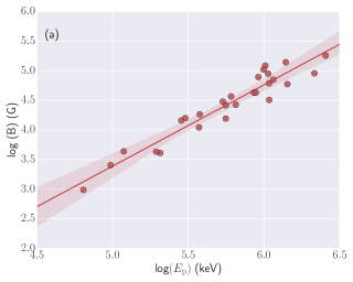
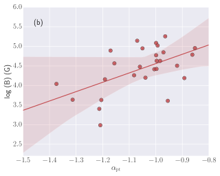
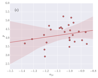
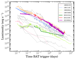
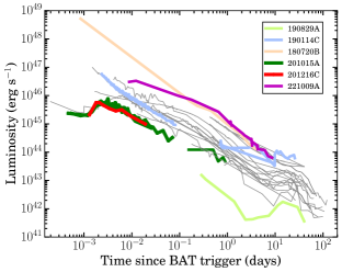
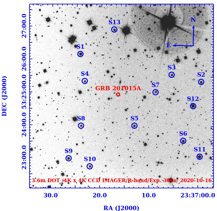
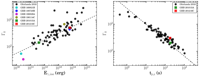
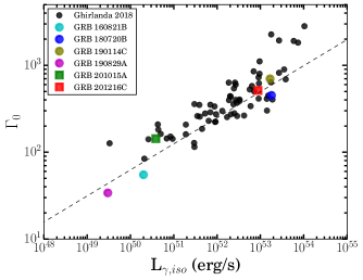
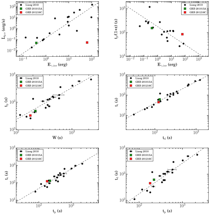
Appendix B Additional Tables
| Model | Spectral parameters | Statistics | |||||
| / () | () | Flux (erg ) | DIC | ||||
| Band | - | 4.29 | 7609.74 | - | |||
| Band+BB | 4.26 | 7502.07 | -107.67 | ||||
| CPL | - | - | 3.38 | 7684.57 | - | ||
| CPL+BB | - | 3.45 | 7558.00 | -126.57 | |||
| Synchrotron | B (G) | Flux (erg ) | DIC | ||||
| - | 4.11 | 7454.89 | - | ||||
| S | CPL | CPL+BB | CPL | CPL+BB | |||||||
| tstart-tstop | Flux | kT | Flux | DIC | DIC | DIC | |||||
| (s) | () | () | () | ||||||||
| 3.93-5.68 | 40.93 | 2.42 | 2.68 | 2394.02 | 2365.42 | -28.6 | |||||
| 5.68-6.23 | 35.83 | 5.2 | 5.73 | 665.66 | 637.12 | -28.54 | |||||
| 6.23-7.24 | 63.53 | 8.08 | 8.36 | 1739.16 | 1719.61 | -19.55 | |||||
| 7.24-10.19 | 120.81 | 7.21 | 7.43 | 3437.91 | 3396.15 | -41.76 | |||||
| 10.19-11.02 | 46.78 | 3.21 | 3.32 | 1256.32 | 1242.7 | -13.63 | |||||
| 11.02-14.90 | 77.15 | 2.15 | 2.19 | 3505.93 | 3491.02 | -14.91 | |||||
| 14.90-15.66 | 48.58 | 3.92 | 4.21 | 1227.59 | 1214.58 | -13.02 | |||||
| 15.66-17.28 | 59.96 | 2.35 | 2.61 | 2286.17 | 2267.03 | -19.14 | |||||
| 17.74-18.58 | 48.27 | 3.22 | 3.31 | 1236.56 | 1229.42 | -7.15 | |||||
| 18.58-19.87 | 73.73 | 5.27 | 5.44 | 2005.36 | 1995.71 | -9.65 | |||||
| 19.87-20.47 | 62.39 | 7.57 | 8.36 | 1052.87 | 1028.02 | -24.85 | |||||
| 20.47-21.42 | 61.86 | 4.06 | 4.36 | 1480.71 | 1468.67 | -12.04 | |||||
| 21.42-21.72 | 44.21 | 7.55 | 7.95 | 13.17 | 7.63 | -5.53 | |||||
| 21.72-22.92 | 61.99 | 3.25 | 3.28 | 1845.48 | 1837.52 | -7.96 | |||||
| 22.92-23.85 | 76.31 | 6.35 | 6.46 | 1581.2 | 1573.82 | -7.38 | |||||
| 23.85-24.28 | 76.51 | 1.17 | 1.19 | 638.32 | 634.18 | -4.14 | |||||
| 24.28-24.73 | 66.46 | 8.69 | 9.39 | 621.01 | 598.12 | -22.88 | |||||
| 24.73-25.83 | 123.46 | 1.24 | 1.33 | 2082.07 | 2047.75 | -34.32 | |||||
| 25.83-27.53 | 134.88 | 9.58 | 9.92 | 2664.38 | 2650.17 | -14.21 | |||||
| 27.53-28.15 | 97.35 | 1.28 | 1.36 | 1248.52 | 1229.01 | -19.51 | |||||
| 28.15-29.06 | 97.18 | 8.29 | 8.95 | 1679.26 | 1654.19 | -25.07 | |||||
| 29.06-29.79 | 69.43 | 4.71 | 5.06 | 1202.71 | 1182.16 | -20.56 | |||||
| 29.79-30.81 | 63.57 | 3.2 | 3.4 | 1659.75 | 1647.92 | -11.83 | |||||
| 30.81-31.95 | 50.74 | 2.29 | 2.35 | 1649.24 | 1645.29 | -3.95 | |||||
| 31.95-33.11 | 39.54 | 1.34 | 1.43 | 1644.47 | 1635.39 | -9.08 | |||||
| 33.11-35.71 | 43.68 | 1.01 | 1.16 | 2812.15 | 2795.55 | -16.6 | |||||
| 35.71-38.83 | 35.6 | 6.66 | 7.35 | 3034.54 | 3022.18 | -12.36 | |||||
| Band | Band+BB | Band | Band+BB | |||||||||
|---|---|---|---|---|---|---|---|---|---|---|---|---|
| tstart-tstop | Flux | Flux | DIC | DIC | ||||||||
| (s) | () | () | () | |||||||||
| 3.93-5.68 | 2.78 | 2.86 | 2391.24 | 2380.36 | -10.88 | |||||||
| 5.68-6.23 | 5.48 | 5.81 | 665.42 | 650.85 | -14.57 | |||||||
| 6.23-7.24 | 1.01 | 1.03 | 1720.89 | 1712.18 | -8.71 | |||||||
| 7.24-10.19 | 9.12 | 9.03 | 3412.17 | 3384.55 | -27.62 | |||||||
| 10.19-11.02 | 3.46 | 3.49 | 1254.32 | 1246.93 | -7.39 | |||||||
| 11.02-14.90 | 2.66 | 2.6 | 3496.97 | 3486.73 | -10.24 | |||||||
| 14.90-15.66 | 4.63 | 4.75 | 1222.70 | 1218.13 | -4.57 | |||||||
| 15.66-17.28 | 3.13 | 3.07 | 2277.67 | 2274.30 | -3.37 | |||||||
| 17.74-18.58 | 3.49 | 3.51 | 1234.22 | 1228.86 | -5.36 | |||||||
| 18.58-19.87 | 6.54 | 6.53 | 1997.41 | 1992.54 | -4.87 | |||||||
| 19.87-20.47 | 9.79 | 9.42 | 1042.53 | 1027.14 | -15.39 | |||||||
| 20.47-21.42 | 4.49 | 4.58 | 1477.02 | 1470.68 | -6.34 | |||||||
| 21.42-21.72 | 9.45 | 9.79 | 7.15 | 2.77 | -4.38 | |||||||
| 21.72-22.92 | 3.59 | 3.56 | 1842.93 | 1836.55 | -6.38 | |||||||
| 22.92-23.85 | 6.69 | 6.68 | 1580.47 | 1574.85 | -5.62 | |||||||
| 23.85-24.28 | 1.31 | 1.32 | 632.94 | 630.25 | -2.69 | |||||||
| 24.28-24.73 | 1.08 | 1.05 | 612.58 | 599.65 | -12.92 | |||||||
| 24.73-25.83 | 1.54 | 1.52 | 2056.01 | 2039.19 | -16.82 | |||||||
| 25.83-27.53 | 1.03 | 1.03 | 2658.61 | 2651.25 | -7.36 | |||||||
| 27.53-28.15 | 1.47 | 1.47 | 1241.25 | 1227.12 | -14.13 | |||||||
| 28.15-29.06 | 9.17 | 9.36 | 1674.67 | 1652.97 | -21.70 | |||||||
| 29.06-29.79 | 6.00 | 5.5 | 1192.50 | 1179.51 | -13.00 | |||||||
| 29.79-30.81 | 4.63 | 4.14 | 1645.06 | 1641.88 | -3.18 | |||||||
| 30.81-31.95 | 2.55 | 2.6 | 1644.99 | 1642.27 | -2.73 | |||||||
| 31.95-33.11 | 1.49 | 1.52 | 1640.42 | 1635.42 | -5.00 | |||||||
| 33.11-35.71 | 1.15 | 1.18 | 2808.19 | 2803.98 | -4.21 | |||||||
| 35.71-38.83 | 8.68 | 8.03 | 2984.82 | 3020.93 | 36.11 |
| tstart-tstop | S | Synchrotron | ||||
|---|---|---|---|---|---|---|
| (s) | B (G) | () | Flux | DIC | ||
| 3.93-5.68 | 40.93 | 3.04 | 1061.27 | |||
| 5.68-6.23 | 35.83 | 6.07 | 495.69 | |||
| 6.23-7.24 | 63.52 | 1.06 | 268.10 | |||
| 7.24-10.19 | 120.80 | 8.87 | 3220.77 | |||
| 10.19-11.02 | 46.78 | 3.75 | 1135.13 | |||
| 11.02-14.90 | 77.15 | 2.58 | 3337.24 | |||
| 14.90-15.66 | 48.57 | 4.88 | -1025.49 | |||
| 15.66-17.28 | 59.95 | 2.93 | 976.25 | |||
| 17.74-18.58 | 48.27 | 3.82 | 1114.54 | |||
| 18.58-19.87 | 73.72 | 6.71 | 1662.13 | |||
| 19.87-20.47 | 62.38 | 9.67 | -617.38 | |||
| 20.47-21.42 | 61.86 | 4.8 | 1357.23 | |||
| 21.42-21.72 | 44.21 | 1.01 | -1935.17 | |||
| 21.72-22.92 | 61.99 | 3.79 | 1789.03 | |||
| 22.92-23.85 | 76.31 | 7.29 | 1566.58 | |||
| 23.85-24.28 | 76.51 | 1.38 | 262.16 | |||
| 24.28-24.73 | 66.46 | 1.06 | -545.52 | |||
| 24.73-25.83 | 123.46 | 1.52 | 1984.83 | |||
| 25.83-27.53 | 134.88 | 1.12 | 2643.94 | |||
| 27.53-28.15 | 97.34 | 1.55 | 1192.78 | |||
| 28.15-29.06 | 97.18 | 9.80 | 1629.70 | |||
| 29.06-29.79 | 69.43 | 5.62 | -6121.04 | |||
| 29.79-30.81 | 63.56 | 4.39 | -11527.37 | |||
| 30.81-31.95 | 50.73 | 2.62 | 1527.57 | |||
| 31.95-33.11 | 39.54 | 1.53 | -310.89 | |||
| 33.11-35.71 | 43.67 | 1.16 | 2521.27 | |||
| 35.71-38.83 | 35.60 | 8.61 | -3405.36 | |||
| Model | Spectral parameters | ||||
|---|---|---|---|---|---|
| / () | () | Flux (erg ) | |||
| Band | - | (6.50 4.08) | |||
| Band+BB | (6.48 4.07) | ||||
| CPL | - | - | (5.50 3.45) | ||
| CPL+BB | - | (5.81 3.63) | |||
| Synchrotron | B (G) | Flux (erg ) | |||
| - | (6.71 4.21) | ||||
| Model | log (Flux)-log () | log (Flux)- | log ()- | log (Flux)-k | ||||
| r | p | r | p | r | p | r | p | |
| Band | 0.79 | 7.19 | 0.60 | 9.67 | 0.65 | 2.11 | - | - |
| Band+BB | 0.83 | 7.75 | 0.53 | 4.13 | 0.56 | 2.39 | 0.72 | 2.51 |
| log (Flux)-log (B) | log (Flux)- | log (B)- | ||||||
| r | p | r | p | r | p | |||
| Synchrotron | 0.80 | 5.43 | 0.31 | 1.10 | 0.54 | 3.53 | ||
| log ()-log (B) | log (B)- | - | ||||||
| r | p | r | p | r | p | |||
| Band-Synchrotron | 0.96 | 5.14 | 0.55 | 3.23 | 0.24 | 2.31 | ||
| ID | U | B | V | R | I |
|---|---|---|---|---|---|
| 1 | 17.750.14 | 16.810.02 | 15.630.00 | 14.940.01 | 14.290.04 |
| 2 | 17.580.14 | 17.190.02 | 16.340.01 | 15.820.01 | 15.350.04 |
| 3 | 17.950.14 | 17.720.02 | 17.000.01 | 16.550.01 | 16.140.04 |
| 4 | 18.460.14 | 18.060.02 | 17.190.01 | 16.660.01 | 16.140.04 |
| 5 | 17.500.14 | 17.280.02 | 16.590.01 | 16.150.01 | 15.750.04 |
| 6 | 17.160.14 | 16.790.02 | 16.000.01 | 15.530.01 | 15.100.04 |
| 7 | 18.110.14 | 17.860.02 | 17.060.01 | 16.550.01 | 16.110.04 |
| 8 | 18.300.14 | 17.760.02 | 16.890.01 | 16.340.01 | 15.860.04 |
| 9 | 17.180.14 | 16.770.02 | 15.940.01 | 15.430.01 | 14.980.04 |
| 10 | 17.790.14 | 17.400.02 | 16.540.01 | 16.020.01 | 15.550.04 |
| 11 | 15.900.14 | 15.690.02 | 15.070.00 | 14.690.01 | 14.360.04 |
| 12 | 18.250.14 | 16.600.02 | 15.140.00 | 14.330.01 | 13.540.04 |
| 13 | 17.830.14 | 17.490.02 | 16.630.01 | 16.040.01 | 15.490.04 |
| time (s) | Exp time (s) | filter | Telescope | Magnitude | Reference |
| 46.65 | 20 | C | FRAM-ORM | 17.49 0.19 | Present work |
| 72.57 | 20 | C | FRAM-ORM | 17.71 0.22 | Present work |
| 100.22 | 20 | C | FRAM-ORM | 17.61 0.20 | Present work |
| 126.14 | 20 | C | FRAM-ORM | 17.37 0.18 | Present work |
| 152.92 | 20 | C | FRAM-ORM | 16.86 0.10 | Present work |
| 178.84 | 20 | C | FRAM-ORM | 16.73 0.09 | Present work |
| 204.76 | 20 | C | FRAM-ORM | 16.67 0.09 | Present work |
| 230.68 | 20 | C | FRAM-ORM | 16.72 0.09 | Present work |
| 256.60 | 20 | C | FRAM-ORM | 16.73 0.10 | Present work |
| 283.39 | 20 | C | FRAM-ORM | 16.96 0.12 | Present work |
| 309.31 | 20 | C | FRAM-ORM | 16.74 0.10 | Present work |
| 335.23 | 20 | C | FRAM-ORM | 16.63 0.09 | Present work |
| 361.15 | 20 | C | FRAM-ORM | 16.90 0.11 | Present work |
| 387.07 | 20 | C | FRAM-ORM | 16.67 0.09 | Present work |
| 412.99 | 20 | C | FRAM-ORM | 16.79 0.10 | Present work |
| 438.91 | 20 | C | FRAM-ORM | 16.77 0.11 | Present work |
| 464.83 | 20 | C | FRAM-ORM | 16.75 0.10 | Present work |
| 490.75 | 20 | C | FRAM-ORM | 16.93 0.12 | Present work |
| 516.67 | 20 | C | FRAM-ORM | 17.01 0.13 | Present work |
| 542.59 | 20 | C | FRAM-ORM | 17.09 0.14 | Present work |
| 605.66 | 98 | C | FRAM-ORM | 17.40 0.09 | Present work |
| 709.34 | 98 | C | FRAM-ORM | 17.64 0.09 | Present work |
| 813.88 | 98 | C | FRAM-ORM | 17.65 0.09 | Present work |
| 917.56 | 98 | C | FRAM-ORM | 17.95 0.12 | Present work |
| 1022.11 | 98 | C | FRAM-ORM | 18.19 0.15 | Present work |
| 40.60 | 11 | C | BOOTES-1B | 17.49 0.47 | Present work |
| 103.68 | 30 | C | BOOTES-1B | 17.68 0.52 | Present work |
| 162.43 | 15 | C | BOOTES-1B | 16.59 0.29 | Present work |
| 194.40 | 10 | C | BOOTES-1B | 16.41 0.35 | Present work |
| 221.18 | 10 | C | BOOTES-1B | 16.58 0.38 | Present work |
| 247.10 | 10 | C | BOOTES-1B | 16.54 0.37 | Present work |
| 273.88 | 10 | C | BOOTES-1B | 16.20 0.30 | Present work |
| 304.12 | 14 | C | BOOTES-1B | 17.04 0.49 | Present work |
| 329.18 | 10 | C | BOOTES-1B | 16.96 0.31 | Present work |
| 340.41 | 10 | C | BOOTES-1B | 16.69 0.25 | Present work |
| 351.64 | 10 | C | BOOTES-1B | 16.71 0.25 | Present work |
| 362.88 | 10 | C | BOOTES-1B | 17.12 0.34 | Present work |
| 374.97 | 10 | C | BOOTES-1B | 17.09 0.32 | Present work |
| 386.20 | 10 | C | BOOTES-1B | 16.55 0.23 | Present work |
| 398.30 | 10 | C | BOOTES-1B | 16.57 0.23 | Present work |
| 408.67 | 10 | C | BOOTES-1B | 16.97 0.29 | Present work |
| 420.76 | 10 | C | BOOTES-1B | 16.89 0.28 | Present work |
| 432.00 | 10 | C | BOOTES-1B | 17.07 0.34 | Present work |
| 444.09 | 10 | C | BOOTES-1B | 16.78 0.26 | Present work |
| 455.32 | 10 | C | BOOTES-1B | 17.09 0.33 | Present work |
| 467.42 | 10 | C | BOOTES-1B | 17.19 0.36 | Present work |
| 477.79 | 10 | C | BOOTES-1B | 16.90 0.28 | Present work |
| 500.25 | 30 | C | BOOTES-1B | 18.20 0.64 | Present work |
| 535.68 | 30 | C | BOOTES-1B | 17.39 0.30 | Present work |
| 569.37 | 30 | C | BOOTES-1B | 16.98 0.23 | Present work |
| 604.80 | 30 | C | BOOTES-1B | 16.99 0.24 | Present work |
| 650.59 | 50 | C | BOOTES-1B | 17.51 0.29 | Present work |
| 707.61 | 50 | C | BOOTES-1B | 17.07 0.22 | Present work |
| 764.64 | 50 | C | BOOTES-1B | 17.50 0.29 | Present work |
| 851.90 | 100 | C | BOOTES-1B | 17.75 0.27 | Present work |
| 966.81 | 100 | C | BOOTES-1B | 17.70 0.28 | Present work |
| 1080.86 | 100 | C | BOOTES-1B | 17.87 0.30 | Present work |
| 1195.77 | 100 | C | BOOTES-1B | 17.89 0.31 | Present work |
| 1368.57 | 200 | C | BOOTES-1B | 18.22 0.50 | Present work |
| 1656.28 | 300 | C | BOOTES-1B | 18.08 0.21 | Present work |
| 2016.57 | 300 | C | BOOTES-1B | 18.60 0.26 | Present work |
| 2399.32 | 300 | C | BOOTES-1B | 18.72 0.16 | Present work |
| 2928.09 | 600 | C | BOOTES-1B | 19.24 0.21 | Present work |
| 3889.72 | 900 | C | BOOTES-1B | 19.01 0.24 | Present work |
| 5011.20 | 900 | C | BOOTES-1B | 19.92 0.32 | Present work |
| 6096.38 | 840 | C | BOOTES-1B | 19.63 0.27 | Present work |
| 72316.80 | 300 | I | DOT | 21.88 0.09 | Present work |
| 52099.20 | 300 | R | DOT | 22.14 0.08 | Present work |
| 73008.00 | 300 | R | DOT | 21.94 0.12 | Present work |
| 52790.40 | 300 | V | DOT | 22.70 0.08 | Present work |
| 73267.20 | 300 | V | DOT | 22.63 0.09 | Present work |
| 74217.60 | 300 | B | DOT | 23.31 0.10 | Present work |
| time (s) | Exposure (s) | Filter | Telescope | Magnitude | Reference |
|---|---|---|---|---|---|
| 47.410 | 20 | C | FRAM-ORM | 18.339 0.295 | Present work |
| 73.770 | 20 | C | FRAM-ORM | 18.38 | Present work |
| 112.40 | 45 | C | FRAM-ORM | 19.101 0.421 | Present work |
| 154.26 | 20 | C | FRAM-ORM | 18.036 0.251 | Present work |
| 180.23 | 20 | C | FRAM-ORM | 18.034 0.253 | Present work |
| 218.19 | 46 | C | FRAM-ORM | 18.269 0.252 | Present work |
| 293.39 | 98 | C | FRAM-ORM | 18.563 0.247 | Present work |
| 398.52 | 98 | C | FRAM-ORM | 18.775 0.299 | Present work |
| 526.91 | 150 | C | FRAM-ORM | 18.665 0.239 | Present work |
| 813.95 | 467 | C | FRAM-ORM | 19.226 0.227 | Present work |
| 1643.47 | 21x60 | R | FRAM-ORM | 19.927 0.346 | Present work |
| 7884.00 | 3x40 | r | VLT | 21.81 0.05 | Izzo et al. (2020) |
| GRB 201015A | |||||||
| Time interval (s) | Spectral regime | Medium | |||||
| 3300 - 4800 | - | -1.07 | 2.720.44 | ISM | |||
| (1.0 - 180) | -1.38 | 2.930.38 | ISM | ||||
| GRB 201216C | |||||||
| Time interval (s) | Spectral regime | Medium | |||||
| 2900 - 17000 | - | -0.97 | 2.420.48 | wind | |||