Prolog for Verification, Analysis and Transformation Tools

Prolog’s non-determinism is of course very convenient when modelling non-deterministic specification languages. Operational semantic rules can often be translated to Prolog clauses. Take, for example, these two inference rules for a prefix operator $\rightarrow$ and an interleaving operator $\|$ in a process algebra inspired by CSP, where $X\stackrel{{\scriptstyle a}}{{\leadsto}}X^{\prime}$ means that the process $X$ can execute the action $a$ and then behave like the process $X^{\prime}$:

These rules can be encoded in Prolog as follows, where trans/3 encodes the ternary semantics relation $\leadsto$:

  trans(’->’(A,Y),A,Y).
  trans(’||’(X,Y),A,’||’(X2,Y)) :- trans(X,A,X2).
  trans(’||’(X,Y),A,’||’(X,Y2)) :- trans(Y,A,Y2).

We can then determine that the process $a\rightarrow stop\|b\rightarrow stop$ can perform two possible actions:

| ?- trans(’||’(’->’(a,stop),’->’(b,stop)),A,R).
A = a,
R = ’||’(stop,(b->stop)) ? ;
A = b,
R = ’||’((a->stop),stop) ? ;
no

We can also compute the two possible traces of length two:

| ?- trans(’||’(’->’(a,stop),’->’(b,stop)),A1,_R1), trans(_R1,A2,R2).
A1 = a,
A2 = b,
R2 = ’||’(stop,stop) ? ;
A1 = b,
A2 = a,
R2 = ’||’(stop,stop) ?
yes

It is quite straightforward to perform exhaustive model checking for such specifications in Prolog, in particular if we have access to tabling (aka memoization) to detect repeated reachable states (or processes), see, e.g., [35, 28].

However, Prolog’s non-determinism also comes in handy for deterministic imperative languages, when moving from interpretation to analysis. Here is an excerpt of an interpreter for a subset of the Java Bytecode, which I use in my lectures. Every instruction in the Java Bytecode consists of an opcode (one byte), followed by its arguments. Java Bytecode uses an operand stack to store arguments to operators and to push results of operators. For example, the imul opcode removes the topmost (integer) values from the stack an pushes the result of the multiplication back onto the stack.¹¹1Java Bytecode is thus also zero-address-code, as such instructions do not take arguments: they implicitly know where the operands are and where the result should stored.

The code fragment below shows the code for the iconst opcode to push a constant onto the operator stack, iop to perform a binary arithmetic operation on the two topmost stack elements, dup to duplicate the topmost value on the stack, return to stop a method (and return void), and a conditional if1 which jumps to a given label if an operator (applied to the topmost stack element and a provided constant) returns true.

Every instruction in the Java Bytecdoe consists of an opcode (one byte), followed by its arguments. As mentioned above, imul and iadd take no arguments. However, these opcodes are converted for our interpreter into the generic iop instruction (which obviously does not exist as such in the Java virtual machine) with the operator as argument. A similar grouping of opcodes has been performed for the conditional instruction, e.g., the bytecode instruction ifle 25 gets translated into the Prolog term if1(<=,0,25) for our interpreter. Similarly, opcodes like iconst_2 take no arguments, but in the Prolog representation below this is represented for simplicity as the Prolog term iconst(2). The Java Bytecode object program is represented by instr(PC,Opcode,Size) facts, where PC is the position (in bytes) of the opcode, Opcode the Prolog term describing the opcode, and Size the size in bytes of the opcode (which is needed to determine the position in bytes of the next opcode). This is a small artificial program, which computes 2*2 and then decrements the value until it reaches 0:

    instr(0,iconst(2),1).
    instr(1,iconst(2),1).
    instr(2,iop(*),1).
    instr(3,iconst(-1),1).
    instr(4,iop(+),1).
    instr(5,dup,1).
    instr(6,if1(’>’,0,3),3).
    instr(9,return,0).

The core of the interpreter contains the following clauses.

    interpreter_loop(PC,In,Out) :-
       instr(PC,Opcode,Size),
       NextPC is PC+Size,
       format(’> ~w  ~w  --> ~w~n’,[PC,In,Opcode]),
       ex_opcode(Opcode,NextPC,In,Out).
    ...
    ex_opcode(iconst(Const),NextPC,In,Out) :-
        push(In,Const,Out2),
        interpreter_loop(NextPC,Out2,Out).
    ex_opcode(dup,NextPC,In,Out) :-
        top(In,Top),
        push(In,Top,Out2),
        interpreter_loop(NextPC,Out2,Out).
    ex_opcode(if1(OP,Cst,Label),NextPC,In,Out) :-
        pop(In,RHSVAL1,In2),
        if_then_else(OP,RHSVAL1,Cst,Label,NextPC,In2,Out).
    ex_opcode(iop(OP),NextPC,In,Out) :-
        pop(In,RHSVAL1,In1),
        pop(In1,RHSVAL2,In2),
        ex_op(OP,RHSVAL1,RHSVAL2,Res),
        push(In2,Res,Out2),
        interpreter_loop(NextPC,Out2,Out).
    ex_opcode(return,_,Env,Env).
    ...

    if_then_else(OP,Arg1,Arg2,_TrueLabel,FalseLabel,In,Out) :-
        false_op(OP,Arg1,Arg2),
        interpreter_loop(FalseLabel,In,Out).
    if_then_else(OP,Arg1,Arg2,TrueLabel,_FalseLabel,In,Out) :-
        true_op(OP,Arg1,Arg2),
        interpreter_loop(TrueLabel,In,Out).

    ex_op(*,A1,A2,R) :- R is A1 * A2.
    ex_op(+,A1,A2,R) :- R is A1 + A2.
    ex_op(-,A1,A2,R) :- R is A1 - A2.

    true_op(<=,A1,A2) :- A1 =< A2.
    true_op(>,A1,A2) :- A1 > A2.
    false_op(<=,A1,A2) :- A1 > A2.
    false_op(>,A1,A2) :- A1 =< A2.

    pop(env([X|S],Vars),Top,R) :- !, Top=X,R=env(S,Vars).
    pop(E,_,_) :- print(’*** Could not pop from stack: ’),print(E),nl,fail.

    top(env([X|_],_),X).

    push(env(S,Vars),X,env([X|S],Vars)).

We can execute the interpreter for the above bytecode and an initial empty environment (the environment contains as first argument the stack and as second argument values for local variables, which we do not use here):

| ?- interpreter_loop(0,env([],[]),Out).
> 0  env([],[])  --> iconst(2)
> 1  env([2],[])  --> iconst(2)
> 2  env([2,2],[])  --> iop(*)
> 3  env([4],[])  --> iconst(-1)
> 4  env([-1,4],[])  --> iop(+)
> 5  env([3],[])  --> dup
> 6  env([3,3],[])  --> if1(>,0,3)
> 3  env([3],[])  --> iconst(-1)
> 4  env([-1,3],[])  --> iop(+)
> 5  env([2],[])  --> dup
> 6  env([2,2],[])  --> if1(>,0,3)
> 3  env([2],[])  --> iconst(-1)
> 4  env([-1,2],[])  --> iop(+)
> 5  env([1],[])  --> dup
> 6  env([1,1],[])  --> if1(>,0,3)
> 3  env([1],[])  --> iconst(-1)
> 4  env([-1,1],[])  --> iop(+)
> 5  env([0],[])  --> dup
> 6  env([0,0],[])  --> if1(>,0,3)
> 9  env([0],[])  --> return
Out = env([0],[]) ?
yes

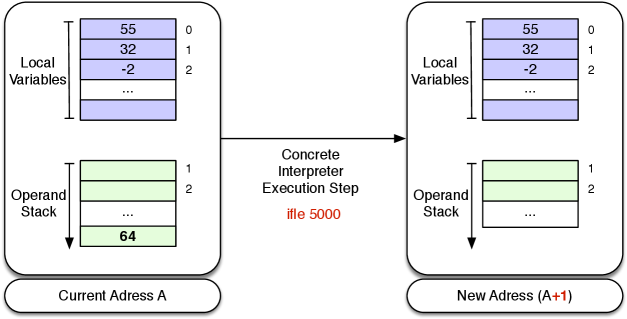
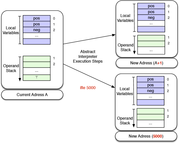
As you can see, the above interpreter is deterministic: when given a state and an opcode it will compute just one solution for the successor state after execution of the opcode. In Prolog one can easily transform such an interpreter into an analysis tool, for either data flow analysis [2] or abstract interpretation [12]. In that case the Prolog program becomes non-deterministic. For example, to transform the above interpreter into an abstract interpreter, one has to define abstract operations, such as an abstract multiplication or an abstract “less or equal” test, over some abstract domain. The abstract domain here contains the following abstract values:

• •

  pos to stand for the positive integers

• •

  neg to denote the negative integers

• •

  0 to denote the single value 0

• •

  top to denote all integers

The bottom value is not needed here in the Prolog interpreter; it is represented implicitly by Prolog failure of the interpreter.

    ex_op(*,0,_,0).
    ex_op(*,pos,X,X).
    ex_op(*,neg,0,0).
    ex_op(*,neg,pos,neg).
    ex_op(*,neg,neg,pos).
    ex_op(*,neg,top,top).
    ex_op(*,top,0,0).
    ex_op(*,top,X,top) :- X\=0.

    ex_op(+,0,X,X).
    ex_op(+,pos,0,pos).
    ex_op(+,pos,pos,pos).
    ex_op(+,pos,neg,top).
    ex_op(+,pos,top,top).
    ex_op(+,neg,0,neg).
    ex_op(+,neg,pos,top).
    ex_op(+,neg,neg,neg).
    ex_op(+,neg,top,top).
    ex_op(+,top,_,top).

    true_op(<=,X,X).
    true_op(<=,top,X) :- X \= top.
    true_op(<=,neg,X) :- X \= neg.
    true_op(<=,0,pos).
    true_op(<=,0,top).
    true_op(<=,pos,top).

    true_op(>,_,top).
    true_op(>,_,neg).
    true_op(>,pos,0).
    true_op(>,top,0).
    true_op(>,pos,pos).
    true_op(>,top,pos).

    false_op(<=,A1,A2) :- true_op(>,A1,A2).
    false_op(>,A1,A2)  :- true_op(<=,A1,A2).

For example, both the call test_op(<=,pos,pos) and false_op(<=,pos,pos) succeeds, and the if_then_else predicate becomes non-deterministic. This is illustrated in Figures 2 and 2 for an opcode ifle 5000, which would be encoded if1(<=,0,5000) in our Prolog interpreter.

To run our interpreter, we first need to use an abstract version of our bytecode program:

    instr(0,iconst(pos),1).
    instr(1,iconst(pos),1).
    instr(2,iop(*),1).
    instr(3,iconst(neg),1).
    instr(4,iop(+),1).
    instr(5,dup,1).
    instr(6,if1(’>’,0,3),3).
    instr(9,return,0).

We can now run the same query as above. This time there are infinitely many solutions (paths) through our program. We show the first three:

 | ?- interpreter_loop(0,env([],[]),R).
> 0  env([],[])  --> iconst(pos)
> 1  env([pos],[])  --> iconst(pos)
> 2  env([pos,pos],[])  --> iop(*)
> 3  env([pos],[])  --> iconst(neg)
> 4  env([neg,pos],[])  --> iop(+)
> 5  env([top],[])  --> dup
> 6  env([top,top],[])  --> if1(>,0,3)
> 9  env([top],[])  --> return
R = env([top],[]) ? ;
> 3  env([top],[])  --> iconst(neg)
> 4  env([neg,top],[])  --> iop(+)
> 5  env([top],[])  --> dup
> 6  env([top,top],[])  --> if1(>,0,3)
> 9  env([top],[])  --> return
R = env([top],[]) ? ;
> 3  env([top],[])  --> iconst(neg)
> 4  env([neg,top],[])  --> iop(+)
> 5  env([top],[])  --> dup
> 6  env([top,top],[])  --> if1(>,0,3)
> 9  env([top],[])  --> return
R = env([top],[]) ?

To transform the interpreter into a terminating abstract interpreter one would still need to store visited program points and corresponding abstract environments and perform the least upper bound of all abstract environments for any given program point (this could be done in the interpreter_loop predicate).

You may have noticed that in the above concrete interpreter, the ifthenelse predicate was not using Prolog negation \+ or the Prolog if-then-else ( Tst -> Thn ; Els), but used a predicate true_op for a successful comparison operator and false_op for a failed comparison. Indeed, the use of the Prolog negation would have prevented the transition from the concrete to the abstract interpreter.

In fact, is rarely a good idea to use Prolog negation to represent negation of the language being analysed. The reason is that Prolog’s built-in negation is not logical negation but so-called “negation-as-failure”. This negation can be given a logical description only when its arguments contain no logical variables at the moment it is called. To understand this issue let us examine a simpler program:

    int(0).
    int(s(X)) :- int(X).

Below are three queries, to this program:

     ?- \+ int(a).   /* succeeds */
     ?- \+ int(X), X=a.  /* fails */
     ?- X=a, \+ int(X).  /* succeeds */

As you can see in the last two queries, conjunction is not commutative here and the Prolog negation is not declarative, i.e., it cannot be described within logic (where conjunction is commutative). More importantly, you can see that the query int(X) fails: we cannot use Prolog’s negation to find values which make a predicate false. This is what we required in the abstract interpreter above: find values which lead to a comparison operator to fail and lead to alternate paths through the bytecode program.

To safely use negation (inside an interpreter) there are basically four solutions. The first is to always ensure that there are no variables when we call the Prolog negation. This may be difficult to achieve in some circumstances; and generally means we can use the interpreter in only one specific way. For our abstract interpreter above, this means that we cannot use the interpreter to find values and computation paths which lead to a comparison operator to fail.

The second solution is to delay negated goals until they become ground. This can be achieved using the built-in predicate when/2 of Prolog. The call when(Cond,Call) waits until the condition Cond becomes true, at which point Call is executed. While Call can be any Prolog goal, Cond can only use: nonvar(X), ground(X), ?=(X,Y), as well as combinations thereof combined with conjunction (,) and disjunction (;). With this built-in we can implement a safe version of negation, which will ensure that the Prolog negation is only called when no variables are left inside the negated call:

  safe_not(P) :- when(ground(P), \+(P)).

A disadvantage of this approach are refutations which lead to a so-called floundering goal, where all goals suspend. In that case, one does not know whether the query is a logical consequence of the program or not. The Gödel programming language [18] supported such a safe version of negation. For program analysis tools, however, we again have the problem that we cannot use this kind of negation to find values for variables.

A third solution is to move to another negation, e.g., constructive negation, or well-founded or stable model semantics and the associated negation. This is available, e.g., in answer-set programming [30] but not in the mainstream Prolog systems.

Finally, the best solution is to circumvent this problem all together, and use no negation at all. Here we do this by explicitly writing a predicate for negated formulas. This is what we have done above, in the form of the predicates true_op and false_op. Below is an illustration of this approach for a small interpreter for propositional logic:

    int(const(true)).
    int(and(X,Y)) :- int(X), int(Y).
    int(or(X,Y)) :- int(X) ; int(Y).
    int(not(X)) :- neg_int(X).

    neg_int(const(false)).
    neg_int(and(X,Y)) :- neg_int(X) ; neg_int(Y).
    neg_int(or(X,Y)) :- neg_int(X),neg_int(Y).
    neg_int(not(X)) :- int(X).

This interpreter now works as expected for negation and partially instantiated queries:

    | ?- int(not(const(X))).
    X = false ? ;
    no

This interpreter thus actively searches for solutions to the negated formulas. This technique is used within the ProB system to handle negation in the B specification language. Observe, that had we used Prolog’s negation to define the negation in our object programs as

    int(not(X)) :- \+ int(X).

Unification is often useful for looking up information in a program database and to model semantics rules. For example, in our Java bytecode interpreter above, we can look for conditional jumps to a certain position by unifying with the instruction database:

    | ?- instr(FromPC,if1(_,_,ToPC),_).
    FromPC = 6,
    ToPC = 3 ?
    yes

Sometimes unification is not just useful but essential, e.g., when implementing type inference. Here is a small demo of Hindley-Milner style [31], written in Prolog with DCGs (Definite Clause Grammars [33]). DCGs were initially developed for parsing but are also useful for threading environments in interpreters and in this case type checkers. Note that these two DCG clauses

    t(a,E,E).
    t(b(A,B),In,Out) :- t(A,In,Env),t(B,Env,Out).

We now encode type inference for a small language containing operations (union, intersect) and predicates(in_set) on sets , arithmetic operations (plus) and predicates (gt), as well as logical conjunction (and) and generic equality (eq).

The operators are polymorphic. For example, eq can be applied to integers and sets of values. Similarly, union can be applied to sets of values, but in any given set all values must have the same type. The predicate type(V,Type,In,Out holds if the value V has type Type given the initial type environment In. The output environment may contain additional variables which are henceforth defined.

    type([],set(_)) --> !, [].
    type(union(A,B),set(R)) --> !,type(A,set(R)), type(B,set(R)).
    type(intersect(A,B),set(R)) --> !,type(A,set(R)), type(B,set(R)).
    type(plus(A,B),integer) --> !,type(A,integer), type(B,integer).
    type(in_set(A,B),predicate) --> !,type(A,TA), type(B,set(TA)).
    type(gt(A,B),predicate) --> !,type(A,integer), type(B,integer).
    type(and(A,B),predicate) --> !,type(A,predicate),type(B,predicate).
    type(eq(A,B),predicate) --> !,type(A,TA),type(B,TA).
    type(Nr,integer) --> {number(Nr)},!.
    type([H|T],set(TH)) --> !,type(H,TH), type(T,set(TH)).
    type(ID,TID) --> {identifier(ID)},\+ defined(id(ID,_)),!,
                      add((id(ID,TID))). % creates fresh variable
    type(ID,TID) --> {identifier(ID)},defined(id(ID,TID)),!.
    type(Expr,T,Env,_) :-
                  format(’Type error for ~w (expected: ~w, Env: ~w)~n’,[Expr,T,Env]),fail.

    defined(X,Env,Env) :- member(X,Env).
    add(X,Env,[X|Env]).

    identifier(ID) :- atom(ID), ID \= [].

    type(Expr,Result) :- type(Expr,Result,[],Env), format(’Typing env: ~w~n’,[Env]).

Note that the identifier predicate uses Prolog’s negation implicitly in the form of the \= operator. This is, however, not an issue as the arguments are all ground.

Observe how, e.g., the rule for the union operator requires that the result and each argument (A and B) is of a set type, but it uses unification of the shared variable R to ensure that all elements in all sets have the same type (namely R).

We can use this small program to perform type inference on the following formula

We can correctly determine the types of all variables in a single pass:

    | ?- type(and(eq(union([z],[x,y]),u),gt(z,v)),R).
    Typing env: [id(v,integer),id(u,set(integer)),id(y,integer),id(x,integer),id(z,integer)]
    R = predicate ?
    yes

In some cases, the type inference algorithm will not return a ground type. E.g., here we compute the type of all variables in the formula $x=\emptyset\cup\emptyset$:

    | ?- type(eq(x,union([],[])),R).
    Typing env: [id(x,set(_1631))]
    R = predicate ?
    yes

We see that $x$ is a set, but we do not know what type its elements are. The program can also be used to generate type error messages:

    | ?- type(and(eq(x,1),eq([],x)),R).
    Type error for x (expected: set(_2167), Env: [id(x,integer)])
    no

A more complex version of this interpreter is used successfully for type inference for the B specification language within the ProB validation tool.

While the logical foundations of Prolog — Horn clauses — are very elegant the full Prolog languages contains “darker” areas and features which can only be understood and given meaning when taking the operational semantics of Prolog into account. If you look closely at the example in Section 2.3 above, we used the cut (written as !), combined with a catch-all error clause at the end which always matches, to be able to detect typing errors. The cut here is used to prevent generating type error messages upon backtracking (as the catch-all clause on its own would always be applicable).

In [22] I wrote:

“Sometimes it is good to view Prolog as a dynamic language, and not feel guilty about using the non-ground representation or dynamically asserting or retracting facts. In many circumstances taking these shortcuts will lead in much shorter and faster code, and it is not clear whether the effort in attempting to write a declarative version would be worthwhile.”

When writing verification or analysis tools in Prolog, it is often a good idea to have a declarative core, where all predicates $p$ of arity $n$ satisfy for all terms $a_{\_}1,\ldots,a_{\_}n$ and bindings $\theta$:

• •

  $\forall\theta$. $p(a_{\_}1,...,a_{\_}n),\theta$ $\equiv$ $\theta,p(a_{\_}1,...,a_{\_}n)$ (binding-insensitive)

• •

  $p(a_{\_}1,...,a_{\_}n),\mathit{fail}$ $\equiv$ $\mathit{fail},p(a_{\_}1,...,a_{\_}n)$ (side-effect free)

Here $G\equiv H$ means that $G$ and $H$ have the same meaning. Usually, this means the same sets of computed answers us

For the infrastructure code (e.g., command-line interface, input-output), it is fine or even mandatory to use impure features of Prolog. For the core of a tool it is also sometimes advisable to use impure features, albeit in a limited fashion. We should strive to keep the predicates declarative in the absence of error messages. E.g., as shown in the type-inference program, we can use the non-declarative cut combined with a catch-all to generate error messages, but the cut did not affect regular type inference.

Co-routines are a mechanism to influence the selection rule of Prolog: via when or block annotations one can suspend predicate calls until a certain condition is met.²²2A suspended goal is a co-routine; the concept for logic programming dates back to MU Prolog [32]. Co-routines can often help to make predicates more declarative, ensuring that they can be used in multiple directions Sometimes it is even possible to use non-declarative features to write a declarative predicate. This is not really surprising, the declarative predicates of the finite domain constraint logic programming library CLP(FD) [10] of SICStus Prolog [36] are partially implemented in the low-level C-language.

Below is the implementation of a declarative addition predicate. We use both co-routines and non-declarative features to ensure that the predicate can be used in multiple directions, is commutative (but still less powerful than addition in CLP(FD)).

    :- block plus(-,?,-), plus(?,-,-), plus(-,-,?).
    plus(X,Y,R) :- ( var(X) -> X is R-Y
                     ; var(Y) -> Y is R-X
                     ; otherwise -> R is X+Y
                    ).

We have that plus(1,1,X) yields X=2, while, e.g., plus(X,1,4) yields X=3 as solution. The block declarations ensure that the predicate plus delays until at least two of its arguments are known. We can thus even solve the equations $x+y=z\wedge z+1=x\wedge x+10=20$.

     | ?- plus(X,Y,Z), plus(Z,1,X), plus(X,10,20).
    X = 10,
    Y = -1,
    Z = 9 ? ;
    no

The first two calls to plus will initially be suspended, while the third call plus(X,10,20) will be executed, instantiating X to 10. This will unblock the second call plus(Z,1,X), instantiating Z to 9, which in turn will unblock the first call to plus.

I would like to thank Laurent Fribourg for his useful feedback on an earlier version of the article.

References

- [1]
- [2] Alfred V. Aho, Monica S. Lam, Ravi Sethi & Jeffrey D. Ullman (2007): Compilers. Principles, Techniques, and Tools (Second Edition). Addison Wesley.
- [3] Elvira Albert, Puri Arenas, Samir Genaim, Germán Puebla & Damiano Zanardini (2007): Cost Analysis of Java Bytecode. In Rocco De Nicola, editor: ESOP, LNCS 4421, Springer-Verlag, pp. 157–172. Available at http://dx.doi.org/10.1007/978-3-540-71316-6_12.
- [4] Elvira Albert, Samir Genaim & Miguel Gómez-Zamalloa (2007): Heap space analysis for java bytecode. In Greg Morrisett & Mooly Sagiv, editors: ISMM, ACM, pp. 105–116. Available at http://doi.acm.org/10.1145/1296907.1296922.
- [5] Elvira Albert, Miguel Gómez-Zamalloa, Laurent Hubert & Germán Puebla (2007): Verification of Java Bytecode Using Analysis and Transformation of Logic Programs. In Michael Hanus, editor: Proceedings PADL 2007, LNCS 4354, Springer-Verlag, pp. 124–139. Available at http://dx.doi.org/10.1007/978-3-540-69611-7_8.
- [6] K. R. Apt & F. Turini (1995): Meta-logics and Logic Programming. MIT Press.
- [7] Joe Armstrong (2007): A history of Erlang. In Barbara G. Ryder & Brent Hailpern, editors: HOPL, ACM, pp. 1–26. Available at http://doi.acm.org/10.1145/1238844.1238850.
- [8] Jonathan Bowen (1999): Animating the Semantics of VERILOG using Prolog. Technical Report UNU/IIST Technical Report no. 176, United Nations University, Macau.
- [9] Randy Bryant (1992): Symbolic Boolean Manipulation with Ordered Binary-Decision Diagrams. ACM Computing Surveys 24(3), pp. 293–318, 10.1145/42282.46161.
- [10] Mats Carlsson, Greger Ottosson & Björn Carlson (1997): An Open-Ended Finite Domain Constraint Solver. In Hugh Glaser Glaser, Pieter H. Hartel & Herbert Kuchen, editors: Proceedings PLILP’97, LNCS 1292, Springer-Verlag, pp. 191–206. Available at https://doi.org/10.1007/BFb0033845.
- [11] W. Chen & D. S. Warren (1996): Tabled Evaluation with Delaying for General Logic Programs. Journal of the ACM 43(1), pp. 20–74, 10.1016/0304-3975(89)90088-1.
- [12] Patrick Cousot & Radhia Cousot (1992): Abstract Interpretation and Application to Logic Programs. The Journal of Logic Programming 13(2 & 3), pp. 103–179, 10.1016/0743-1066(92)90030-7.
- [13] Berndt Farwer & Michael Leuschel (2004): Model checking object Petri nets in Prolog. In: Proceedings PPDP ’04, ACM Press, New York, NY, USA, pp. 20–31, 10.1145/1013963.1013970.
- [14] Thom Frühwirth (2009): Constraint Handling Rules. Cambridge University Press, 10.1017/CBO9780511609886.
- [15] Miguel Gómez-Zamalloa, Elvira Albert & Germán Puebla (2007): Improving the Decompilation of Java Bytecode to Prolog by Partial Evaluation. Electr. Notes Theor. Comput. Sci. 190(1), pp. 85–101. Available at http://dx.doi.org/10.1016/j.entcs.2007.02.062.
- [16] Sergey Grebenshchikov, Nuno P. Lopes, Corneliu Popeea & Andrey Rybalchenko (2012): Synthesizing software verifiers from proof rules. In Jan Vitek, Haibo Lin & Frank Tip, editors: ACM SIGPLAN Conference on Programming Language Design and Implementation, PLDI ’12, Beijing, China - June 11 - 16, 2012, ACM, pp. 405–416, 10.1145/2254064.2254112. Available at http://dl.acm.org/citation.cfm?id=2254064.
- [17] Patricia Hill & John Gallagher (1998): Meta-programming in logic programming. In D. M. Gabbay, C. J. Hogger & J. A. Robinson, editors: Handbook of Logic in Artificial Intelligence and Logic Programming, 5, Oxford Science Publications, Oxford University Press, pp. 421–497.
- [18] Patricia Hill & John W. Lloyd (1994): The Gödel Programming Language. MIT Press.
- [19] Pieter Hintjens (2013): ZeroMQ: Messaging for Many Applications. O’Reilly Media, Inc.
- [20] Bishoksan Kafle, John P. Gallagher & Pierre Ganty (2018): Tree dimension in verification of constrained Horn clauses. Theory Pract. Log. Program. 18(2), pp. 224–251, 10.1017/S1471068418000030.
- [21] Philipp Körner & Jens Bendisposto (2018): Distributed Model Checking Using ProB. In Aaron Dutle, César A. Muñoz & Anthony Narkawicz, editors: NASA Formal Methods - 10th International Symposium, NFM 2018, Newport News, VA, USA, April 17-19, 2018, Proceedings, Lecture Notes in Computer Science 10811, Springer, pp. 244–260, 10.1007/978-3-319-77935-5_18.
- [22] Michael Leuschel (2008): Declarative Programming for Verification: Lessons and Outlook. In: Proceedings PPDP’2008, ACM Press, pp. 1–7, 10.1145/1389449.1389450.
- [23] Michael Leuschel & Jens Bendisposto (2010): Directed Model Checking for B: An Evaluation and New Techniques. In Jim Davies, Leila Silva & Adenilso da Silva Simão, editors: Formal Methods: Foundations and Applications - 13th Brazilian Symposium on Formal Methods, SBMF 2010, Natal, Brazil, November 8-11, 2010, Revised Selected Papers, Lecture Notes in Computer Science 6527, Springer, pp. 1–16, 10.1007/978-3-642-19829-8_1.
- [24] Michael Leuschel & Michael Butler (2003): ProB: A Model Checker for B. In Keijiro Araki, Stefania Gnesi & Dino Mandrioli, editors: FME 2003: Formal Methods, LNCS 2805, Springer-Verlag, pp. 855–874, 10.1007/978-3-540-45236-2_46.
- [25] Michael Leuschel & Michael J. Butler (2008): ProB: an automated analysis toolset for the B method. STTT 10(2), pp. 185–203. Available at http://dx.doi.org/10.1007/s10009-007-0063-9.
- [26] Michael Leuschel & Marc Fontaine (2008): Probing the Depths of CSP-M: A new FDR-compliant Validation Tool. In: Proceedings ICFEM 2008, LNCS, Springer-Verlag, pp. 278–297, 10.1007/978-3-540-88194-0_18.
- [27] Michael Leuschel & Helko Lehmann (2000): Coverability of Reset Petri Nets and other Well-Structured Transition Systems by Partial Deduction. In John Lloyd, editor: Proceedings of the International Conference on Computational Logic (CL’2000), LNAI 1861, Springer-Verlag, London, UK, pp. 101–115, 10.1007/3-540-44957-4_7.
- [28] Michael Leuschel & Thierry Massart (2000): Infinite State Model Checking by Abstract Interpretation and Program Specialisation. In Annalisa Bossi, editor: Proceedings LOPSTR’99, LNCS 1817, Venice, Italy, pp. 63–82, 10.1007/10720327_5.
- [29] Michael Leuschel, Thierry Massart & Andrew Currie (2001): How to Make FDR Spin: LTL Model Checking of CSP by Refinement. In J. N. Oliviera & P. Zave, editors: FME’2001, LNCS 2021, Springer-Verlag, Berlin, Germany, pp. 99–118, 10.1007/3-540-45251-6_6.
- [30] Victor W. Marek & Miroslaw Truszczynski (1999): Stable Models and an Alternative Logic Programming Paradigm. In Krzysztof R. Apt, Victor W. Marek, Mirek Truszczynski & David Scott Warren, editors: The Logic Programming Paradigm - A 25-Year Perspective, Artificial Intelligence, Springer, pp. 375–398, 10.1007/978-3-642-60085-2_17.
- [31] Robin Milner (1978): A Theory of Type Polymorphism in Programming. Journal of Computer and System Sciences 17, pp. 348–375, 10.1016/0022-0000(78)90014-4.
- [32] Lee Naish (March 1982 (Revised July 1983)): An introduction to MU-Prolog. Technical Report 82/2, Department of Computer Science, University of Melbourne, Melbourne, Australia.
- [33] Fernando C. N. Pereira & David H. D. Warren (1980): Definite Clause Grammars for Language Analysis - A Survey of the Formalism and a Comparison with Augmented Transition Networks. Artif. Intell. 13(3), pp. 231–278, 10.1016/0004-3702(80)90003-X.
- [34] Y. S. Ramakrishna, C. R. Ramakrishnan, I. V. Ramakrishnan, Scott A. Smolka, Terrance Swift & David S. Warren (1997): Efficient Model Checking Using Tabled Resolution. In O. Grumberg, editor: Proceedings CAV’97, LNCS 1254, Springer-Verlag, pp. 143–154, 10.1007/3-540-63166-6_16.
- [35] C. R. Ramakrishnan, I. V. Ramakrishnan, Scott A. Smolka, Yifei Dong, Xiaoqun Du, Abhik Roychoudhury & V. N. Venkatakrishnan (2000): XMC: A Logic-Programming-Based Verification Toolset. In: Proceedings of CAV 2000, pp. 576–580, 10.1007/10722167_48.
- [36] Sweden SICS, Kista: SICStus Prolog User’s Manual. Available at http://www.sics.se/sicstus.