Projection pursuit adaptation on polynomial chaos expansions
Abstract
The present work addresses the issue of accurate stochastic approximations in high-dimensional parametric space using tools from uncertainty quantification (UQ). The basis adaptation method and its accelerated algorithm in polynomial chaos expansions (PCE) were recently proposed to construct low-dimensional approximations adapted to specific quantities of interest (QoI). The present paper addresses one difficulty with these adaptations, namely their reliance on quadrature point sampling, which limits the reusability of potentially expensive samples. Projection pursuit (PP) is a statistical tool to find the “interesting” projections in high-dimensional data and thus bypass the curse-of-dimensionality. In the present work, we combine the fundamental ideas of basis adaptation and projection pursuit regression (PPR) to propose a novel method to simultaneously learn the optimal low-dimensional spaces and PCE representation from given data. While this projection pursuit adaptation (PPA) can be entirely data-driven, the constructed approximation exhibits mean-square convergence to the solution of an underlying governing equation and is thus subject to the same physics constraints. The proposed approach is demonstrated on a borehole problem and a structural dynamics problem, demonstrating the versatility of the method and its ability to discover low-dimensional manifolds with high accuracy with limited data. In addition, the method can learn surrogate models for different quantities of interest while reusing the same data set.
keywords:
Surrogate modeling, polynomial chaos expansion, projection pursuit, high-dimensional models, dimension reduction, data-driven1 Introduction
Recent developments in sensing have enabled highly resolved characterization of physical systems, justifying the drive for computational models of increasingly higher resolution and constantly pushing computational resources to the limit of hardware capacity. This computational bottleneck challenge is further exacerbated when uncertainty is acknowledged, which, at least conceptually, necessitates the simultaneous contemplation of a number of plausible realities. Allowing uncertainty to infiltrate computational models, however, can serve, with the proper perspective, to alleviate the computational burden, allowing consistency between numerical accuracy, statistical confidence, and experimental paucity. Response prediction can thus be achieved with the help of statistical surrogate models, which we achieve in the present paper by augmenting machine learning (ML) paradigms with an uncertainty quantification (UQ) dimension. Typically, these surrogate models are trained on replicas obtained by evaluating the physical model over a set of input parameters. Each of these evaluations will typically involve an expensive high-fidelity model, which is typically described by a large number of parameters. This combination of high resolution and high parameterization continues to challenge the accuracy of surrogate modeling. Similarly, in a big data set, the data of various control variables are generated such that comprehensive information on the quantity of interest (QoI) is considered in the predictive model. Usually, the number of data required for prediction with good accuracy increases with the number of parameters. Surrogate modeling in high-dimensional parameter space is thus ubiquitous, remaining at the forefront of predictive science.
UQ is a tool to characterize the uncertainty in specific responses or outputs, given that the input parameters of the system are uncertain [1, 2, 3, 4, 5, 6, 7]. Generally, the uncertainties in the input parameters are represented by random variables that are characterized by their probability distributions. Usually, the supports of the parameters are first provided. This information is sometimes complemented by marginal distributions for each parameter. Only on rare occasions is joint information on the input parameters available at the outset. Such information may be weaved into the statistical model following data-driven updating. In all cases, the output is computed over a set of input parameters that, in principle, spans the support of their joint probability measure in parameter space. In a standard UQ setting, the probabilistic model of the output can be quantified by propagating the uncertainties from the input space through the computational model. Surrogate models, on the other hand, aim to construct a mapping from input parameters to output variables. The ensuing representation can be used as a surrogate to efficiently map the support of the input parameters into the support and distribution of the quantities of interest. In the literature, it is not uncommon to use UQ models as an efficient surrogate for further analyses that require repeated evaluation of the computational model, for example, in [8, 9, 10, 11]. The quality of these surrogates is clearly paramount. Polynomial chaos representations [1] can be shown to be faithful mathematical representations that converge in the mean-square sense to the true solution of the underlying governing stochastic equations.
For high-dimensional UQ problems, the standard Monte Carlo (MC) sampling has the attractive feature that its convergence is independent of the number of random parameters, thus can avoid the curse-of-dimensionality. However, it has slow convergence in general, and the rate is dependent on the complexity of the solution being sought. Thus the development of UQ methods such as polynomial chaos expansion (PCE) [1, 12], generalized polynomial chaos expansion (gPCE) [13, 14], Gaussian processes [15, 16, 17], probability density evolution methods [18, 19, 7, 6], manifold methods [20, 21, 22], Wiener path integral technique[23, 24], and others. PCE expands the QoI on a set of multivariate Hermite polynomial bases where the approximation has a mean-squared sense convergence with respect to the maximum order or degree of the polynomial bases. Its solid mathematical foundation, accuracy, simplicity in application, and convergence property gained much attention from science and engineering applications [1, 12, 2, 4]. However, the number of PCE terms in the expansion grows factorially with the parameters’ dimension and the maximum polynomial order, leading to the curse-of-dimensionality. In a more common non-intrusive implementation, the PCE coefficients associated with each term are computed as a multi-dimensional integral, where the dimension is equal to the parameters’ dimension. One can typically use numerical quadrature [25, 26] to avoid excessive computation arising from the model evaluation to compute the PCE coefficients. Sparse quadrature [27, 28, 29, 26] can reduce the cost without sacrificing accuracy. Another family of methods, for example, least angle regression [30, 31], and compressive sensing [32, 33, 34], propose a sparse representation by expanding QoI on a selection of significant polynomial bases. These methods attenuate the computational burden but still face challenges if the dimension is excessively large or the computational model is expensive. Active subspace [35, 36] is a dimension reduction technique that finds the important directions with the greatest variability by an eigendecomposition of the covariance matrix of the gradient. In practice, the gradient of the QoI usually takes much work to obtain. The basis adaptation method [37] in the framework of PCE is another dimension reduction technique that finds directions adapted to low-dimensional or scalar QoI. The idea is based on rotating the Gaussian input variables with a proper rotation matrix so that the QoI can be represented in a low-dimensional space. The construction of the rotation matrix requires the first-order PCE coefficients, which can be obtained by a first-order pilot PCE. Basis adaptation has been applied to practical engineering problems [38, 39] that reduce the dimension to only a few. This method can have slow convergence, resulting in relatively high reduced dimensions. Thus, the authors developed the accelerated basis adaptation method [40]. The basis adaptation method requires the construction of low-dimensional adapted PCEs, where the PCE coefficients are usually computed via sparse quadrature to reduce computational cost. In addition, the method is adapted to scalar or low-dimensional QoIs.
In ML, dimension reduction techniques, for example, feature selection [41, 42], matrix factorization [43, 44], manifold learning [45, 46], and autoencoder methods [47, 48], have been able to increase the performance when the dimension of the data is high. Among these, the principal component analysis (PCA) is arguably the most widely used method, useful for discovering components that have ranked importance and can capture the data’s salient structure. Projection pursuit (PP) [49, 50, 51] is another dimension reduction technique used to find the most “interesting” projections in high-dimensional data that can overcome the curse-of-dimensionality. The low-dimensional interesting projections are found by maximizing a so-called projection index stage-wisely. Different definitions of projection index lead to specific methods, for example, PCA and discriminant analysis. PP has received attention in ML in the recent two decades. For example, in [52], new projection indices were proposed to provide low-dimensional projections for efficient supervised classification. For the classification of complex data, a projection pursuit constructive neural network was proposed to discover the simplest models in [53]. Based on the Jensen-Shannon divergence, a supervised projection pursuit was proposed in [54] for better classification and visualization and proved superior to PCA. In [55], PP was used to develop a novel recurrent neural network for discriminant analysis. These works all belong to the scope of the classification. The combination of statistics and ML methods to improve the prediction performance is not unusual, for example, the Bayesian neural networks [56, 57, 58]. One of the extended ideas of PP is the projection pursuit regression (PPR) [59]. In PPR, the response surface is approximated by a sum of univariate smooth functions of linear combinations, represented by projections of the input parameters (or predictors). The projections in PPR are found in a forward stage-wise strategy until new projections cannot improve the approximation significantly. Since the number of projections can be taken arbitrarily large, with a proper choice of smooth functions, the PPR model is able to approximate any continuous function in the space spanned by the parameters [60]. Such a PPR model is thus a universal approximator. PPR has been applied to many practical applications, for example, in [61, 62, 63, 64].
The basis adaptation in PCE and the PPR have many shared features. They find the important or interesting directions in the input parameter space adapted to the output. The rotation matrix in adaptation corresponds to the projections in PPR. In contrast, the PCE of the adapted variables in adaptation corresponds to the smooth functions of the projected variables. However, these two methods are different in several aspects. The rotation matrix in adaptation is constructed based on a first-order PCE, and the directions are mutually orthogonal. At the same time, the projections in PPR are found one at a time, and no restrictions are applied among the projections. In addition, the functional links input parameters to output response in adaptation are Hermite polynomial bases, while in PPR, one must find proper smooth functions suited for the application. Also, the PCE coefficients in adaptation are usually found by sparse numerical quadrature (requiring the evaluation of the model on specific parameters) to reduce the computational cost. In contrast, the projections and smooth functions in PPR are discovered based on given data. Then, the advantages of these two methods can be summarized as follows: (1) the adaptation method uses Hermite polynomial bases that can represent any variable in the parameters space, and it has mean-squared convergence to the maximum polynomial order; (2) the PPR model can find projections and smooth functions simultaneously in a data-driven manner without querying the model.
In this paper, we integrate the basis adaptation method in PCE and the PPR model to take advantage of both methods. Specifically, we use PCEs as smooth functions in the PPR model. In a naive integration, the PCEs work as univariate functions on each projected variable. To take advantage of the completeness and convergence properties of the multivariate Hermite polynomial bases, we will maintain the orthogonality of the projections and use a multivariate PCE on all the projected variables in the approximation. Switching from an additive of many univariate models to a multivariate model, in general, will be less cost-efficient. However, the purpose is to find a low-dimensional representation of the output; thus, the number of projections considered is supposed to be small. In such circumstances, seeking a more accurate multivariate representation is reasonable. We refer to the integrated multivariate model as the projection pursuit adaptation (PPA) model. Note that the projections construct the rotation matrix in the PPA model; thus, the multivariate PCE on the projected variables can be transformed back to the original physical space for interpretation purposes. The proposed model will be compared with the basis adaptation and the PPR methods. The paper is organized as follows: Section 2 introduces the basis adaptation method, including the accelerated algorithm, in the framework of PCE; Section 3 first introduces the detailed procedure of the PPR, then derives the integrated PPA model with a detailed procedure also given; the applications on a borehole model and a space structure are shown in Section 4; conclusions are finally presented in Section 5.
2 Basis adaptation on polynomial chaos expansions
2.1 Polynomial chaos expansions
Consider a probability space with the sample space, the -algebra on , and the probability measure. Let be a set of independent standard Gaussian variables on . Then, the closed linear span (this allows for the case where ) of defines a Gaussian Hilbert space, denoted as . Denoting the space of second order random variables on by , an inner product on can be introduced as
| (1) |
where is the mathematical expectation with respect to the probability measure . Let be a -dimensional multi-index with its length defined as , be multivariate Hermite polynomials, and be the normalized Hermite polynomials, then is a complete orthonormal basis on . We also let denote the -algebra generated by . Then we can represent any random variable as the following polynomial chaos expansion (PCE) [1]
| (2) |
In Eq (2), is the PCE coefficient associated with the basis .
In a computational context, a truncated PCE is usually employed where the maximum order of the polynomials is specified. Suppose the maximum order of the PCE is , then the order PCE of can be written as,
| (3) |
where is the subset of indices of maximum length (i.e., ). The above expression, converges to in the mean-squared sense [65] as . With abuse of notation, we will henceforth use to denote . The total number of PCE terms in Eq (3) is
| (4) |
which grows factorially with the dimension of the parameter space and the maximum order . In a non-intrusive implementation of the PCE [1, 25, 26], the PCE coefficients are computed by projecting on the space spanned by the Hermite polynomial basis (referred to as the original space) as
| (5) |
The projection can be calculated by, for example, the sampling-based Monte Carlo Simulation (MCS). In this setting, a set of samples is evaluated. These samples are then used to estimate the PCE coefficients by minimizing the squared norm of the residual
| (6) |
The optimization problem can be solved by Ordinary Least Squares (OLS). Other methods to choose the sampling set could result in a weighted least squares problem. To obtain a stable and accurate estimation of the PCE coefficients, the number of required samples is typically of order , and in some cases [66]. With the factorial increased with respect to and , the required computation effort becomes prohibitive when the dimension of parameters is high.
Eq (5) can also be approximated using numerical quadrature [26], where the physical model must be evaluated at specific quadrature points. Usually, the required samples could reduce a lot compared to MC samples. The sparse quadrature rules [28, 29, 27] can reduce the required quadrature points by adopting a sparse sampling algorithm. Other methods propose sparse PCE representations where only the dominant PCE terms are considered in the expansion [30, 32, 33, 67]. These methods partially attenuate the computation burden. However, the challenge of the curse-of-dimensionality remains as the underlying physical problem is mixed with high-dimensionality and a complex computational model.
2.2 Basis adaptation
2.2.1 Rotation
Basis adaptation is a dimension reduction technique for PCE in which the Gaussian input variables are rotated by a proper rotation matrix such that the QoI can be represented on a low-dimensional space.
Consider a rotation matrix such that , and let be the rotated variables defined as
| (7) |
where are the first components, and are the remaining components of . Then, instead of expanding with respect to the original variable , we can equivalently represent by the rotated variables as
| (8) |
Same as in the original space, the PCE coefficients can be computed by projecting on the space spanned by (referred to as the rotated space) as
| (9) |
Define
| (10) |
Then, by the equivalence of Eq (3) and Eq (8), we have
| (11) |
The above equation provides the foundation to transfer a PCE model from one representation to another and can be used to compare expansions with respect to different Gaussian variables.
2.2.2 Classical Gaussian adaptation
The rotation changes the variables the QoI expands on without changing the quality of the overall PCE, and without affecting the requisite computational burden. The idea of basis adaptation is to find a proper rotation matrix such that the probabilistic information of the QoI is concentrated on a low-dimensional space to achieve dimension reduction. Therefore, the construction of the rotation matrix becomes crucial.
The rotation matrix is constructed purely based on a first-order PCE expansion on the original space in classical Gaussian adaptation. If the first-order pilot PCE that requires a limited number of model evaluations is constructed, then the rotation matrix is created such that
| (12) |
where is a -dimensional multi-index with one at the th location and zeros elsewhere, then is the set of first-order PCE coefficients or Gaussian coefficients in the original space. Eq (12) defines the first row of the rotation matrix , with which the first rotated variable captures the complete Gaussian components of the QoI. Next, the other rows of are defined based on the sensitivity of the original variables. The sensitivities of the original variables are quantified by the absolute values of their Gaussian coefficients. As a result, the second row of is defined such that is the most sensitive variable of ; the third row of is defined such that is the second most sensitive variable of ; and so on. Finally, a Gram-Schmidt procedure is applied to to make it a rotation matrix. The complete procedure to construct the rotation matrix for the classical basis adaptation is summarized in Algorithm 1.
| (13) |
The Gaussian components are typically the most important information in many applications. Therefore, the first rotated variable conveys the key information of the QoI. Since the other rotated variables are initially constructed as the most sensitive variables in the original space in descending order, the rotated variables have a descending order of importance to the QoI, motivating the seeking of a reduced representation of the QoI by the first several rotated variables. The rows of the rotation matrix are sometimes referred to as the adaptation or adapted directions.
Suppose the first rotated variables are adequate to represent the QoI, , then we can write
| (14) |
where denotes the sub-matrix of the first rows of ; is a set of -dimensional multi-indices. We will refer to Eq (14) as the -dimensional adapted PCE, or simply -dimensional adaptation. The PCE coefficient can be calculated by projecting on the space spanned by the Hermite polynomial basis (referred to as the reduced rotated space) as
| (15) |
Regardless of the methods used to compute Eq (15), the physical model must be evaluated on the original variables instead of . Thus, the following approximation is employed
| (16) |
That is, when projecting back to the original coordinates, we assume that . The assumption introduces negligible errors when the first components of are adequate to capture the probabilistic information of the QoI.
The reduced dimension remains to be determined. A systematic way starts with , where we construct an -dimensional adaptation. Then, is sequentially increased. The procedure is stopped when the difference between two adaptations with successive dimensions is within a pre-specified tolerance. The measure of the difference between two adaptations, such as and dimensional adaptations, can be quantified by the distance of either their PCE coefficients or the associated Kernel Density Estimate (KDE) of the probability density functions (PDF) of the QoI. In the former, the -dimensional adaptation is projected to the -dimensional space, leading to a representation in the -dimensional space (same idea as presented in Eq (11)). The projected PCE coefficients can then be compared to the ones of the -dimensional adaptation. In the latter, many MC samples are first generated based on the constructed - and -dimensional adaptations independently. These MC samples are then used to construct two KDE estimations of the PDF of the QoI, which are then compared to find a quantified difference.
In many applications, the classical basis adaptation can identify low-dimensional spaces adapted to the QoI, for example, [38, 39]. In [40], the authors proposed accelerated basis adaptation methods that can further enhance the accuracy of the reduced dimension . The accelerated algorithm reduces the dimension when the classical adaptation still requires middle-to-high dimensions.
2.2.3 Accelerated adaptation
In [40], two acceleration methods of basis adaptation are proposed. The first method corrects the low-order information of the adapted PCE by utilizing the first-order pilot PCE constructed in the first step of adaptation, see Algorithm 1. The second method updates the rotation matrix by accounting for the information from higher dimensions and high-order adaptations while the dimension is sequentially increased. We will introduce the ideas behind these two methods briefly. For a detailed algorithm, please refer to [40].
Suppose the first-order pilot PCE in the original space is constructed as
| (17) |
Denoting the vector of Gaussian coefficients as , then the -dimensional adaptation of order up to one can be expanded as
| (18) |
To measure the difference in the zero and first-order expansions, the PCE (18) can be projected to the original space to obtain the associated PCE coefficients as
| (19) |
where denotes the component of the rotation matrix . When , the projected coefficients can be computed explicitly as
| (20) |
Defining , then the errors of the Gaussian coefficients are quantified as
| (21) |
We see that the arithmetic errors are proportional to the exact Gaussian coefficients , implying that more significant errors appear in the terms with greater Gaussian coefficients. However, greater Gaussian coefficients imply greater sensitivities in the variable, and greater errors in the terms with greater sensitivity introduce more significant errors in the PCE. As dimension of the adaptation increases, the errors in Gaussian coefficients decrease and will recover to the exact values when . In order to eliminate the errors in the zero and first-order information of the adapted PCE, the authors proposed to correct the zero and first-order PCE coefficients on the adapted space by the exact zero and first-order PCE coefficients on the original space. The idea is accomplished by projecting Eq (17) to the -dimensional adapted space and obtaining the projected coefficients as
| (22) |
These coefficients are the exact zero and first-order PCE coefficients in the -dimensional adapted space and can be used to correct the coefficients in Eq (18). Then, the zero and first-order information are guaranteed to be accurate.
For the second method, we noticed that with the increased in the adaptation, the QoI could be better represented by the adapted PCE. In addition, the -dimensional adapted PCE retains the information of the first rotated variables up to order . However, the rotation matrix in the classical adaptation only considers the first-order information and remains constant even when more probabilistic information becomes available. The second method in [40] proposed to update the rotation matrix as is sequentially increased. Specifically, suppose the -dimensional adaptation from the rotation matrix is available. In that case, the best one-dimensional adaptation close to the -dimensional adaptation is discovered from an updated rotation matrix . The one-dimensional adaptation by can be written as
| (23) |
where is the new adapted variable by . To compute the PCE coefficients of the new one-dimensional adaptation, one would usually require to evaluate the physical model on some parameters. To avoid the additional computation, the evaluation is instead performed on the -dimensional adapted PCE by , the best available model. For any choice of , one can easily construct the one-dimensional adapted PCE of the QoI. Then, an optimization procedure can be employed to find the best that minimizes the difference between the one-dimensional adaptation by and the -dimensional adaptation by . This method can be combined with the first method that always corrects the zero and first-order PCE coefficients in the adapted PCEs. The combined method is named the sequentially optimized adaptation (SOA) with its workflow in Figure 1. Please refer to [40] for details.
The basis adaptation is a great tool for dimension reduction in UQ. However, when it comes to computing the adapted PCE coefficients, for example, by Eq (15), we typically use sparse quadrature rules to reduce the number of evaluations while having good accuracy at the same time. In this setting, the model must be evaluated at specific quadrature points. We will next introduce a novel data-driven method that can simultaneously find the optimal rotation matrix and the PCE coefficients.
3 Projection pursuit adaptation
3.1 Projection pursuit regression
Projection pursuit (PP) intends to find the most “interesting” projections in high-dimensional data. These projections are discovered such that they reveal the most information embedded in the data. Therefore, the projections of PP and the adaptation directions by the basis adaptation method have the same purpose but are discovered with different algorithms. The advantages and disadvantages of these two methods are worth exploring. In the sense of adapting input to output, the projection pursuit regression (PPR) was introduced [59], where the projections and the functions from input space to output space are built simultaneously.
In a general supervised learning setting, assume we have a data set with and . Let , be -dimensional known vectors. Then the PPR model seeks to approximate as follows
| (24) |
where is a set of univariate smooth functions. This model aims to find such that the approximation fits the data in some optimal sense. Specifically, the following optimization problem is solved to fit such a model with the given data
| (25) |
In this optimization problem, the number of required projections, , is determined by a stage-wise greedy algorithm where we add a pair of at each stage and stop the procedure if additional information cannot improve the model fitting significantly. For example, suppose we are in stage and want to find the optimal . Let the previously found parameters, be fixed, then the residual of the th data point is obtained as
| (26) |
Then, the optimal can be found by solving the following optimization problem
| (27) |
When the total residual of the data is converged, we stop the procedure.
An alternative to the greedy procedure is to iteratively update the pairs for through backfitting. While this approach could result in significantly fewer terms in the model, the computation cost is increased, and the improvement in predictions is insignificant [60]. In addition, the same performance can usually be achieved by adding more terms to the model. Therefore, we will focus on the stage-wise greedy procedure.
The optimization problem (27) remains to be solved in each stage. The solution can be obtained by an alternating optimization procedure, where the optimization switches between and until converge. Specifically, if the vector is given, then the argument of is a one-dimensional variable. The problem becomes finding the optimal such that the residual is minimized. This can be done by the regression method. On the other hand, assuming is given, one needs to find the optimal to minimize the residual. This can be done by a Gauss-Newton search, a quasi-Newton method that keeps only the zero and first derivatives in a Taylor expansion. Let be the current estimate of , then we can write the following Taylor expansion
| (28) |
Substituting Eq (28) into Eq (27) (with given) leads to
| (29) |
The optimization problem (29) can be solved by the weighted least squares regression with target , regressors , weight , and no bias term. Let denote the diagonal matrix with entries , be the vector with entries , and use the full data matrix , then is found by solving the following
| (30) |
With an updated , we find new projections and refit to minimize the residual. Then can be updated again with the new . We repeat the alternating procedure until pair is converged.
Although there is no restriction to the smooth functions , it is better if the functions are once differentiable. PCE is a good fit here where each smooth function is a univariate PCE with respect to the projected variable . In this case, the variables that can be arbitrarily distributed (based on prior knowledge or from the data) need to be first transformed to standard Gaussian distributions via, for example, inverse transform sampling or Rosenblatt transformation [68]. Then, with a given , finding the optimal is equivalent to finding the PCE coefficients of . One of the benefits of using PCEs as smooth functions is that the order of the PCE is adjustable, and we can gradually increase the polynomial orders until convergence is reached. Based on the flexibility of PCE, can be arbitrarily large to approximate any function in , and the computational cost lies in constructing univariate PCEs.
Note that there is no restriction on the projection in the optimization problem (30), and each projection is discovered based on the current residual. The initial guess of and the data determine where the “optimal” value land. Therefore, there are chances that the weighted least squares find the local optima and stop the stage-wise procedure when the local optima suggest there is not much room for improvement. In addition, there is no restriction on the projections. No coupling effects are considered among the projections since the smooth function only considers information on the th projected variable. One of the advantages of such construction is that are univariate functions and are easy to compute with given projections and a given number of samples.
3.2 Integration of projection pursuit and basis adaptation
In the basis adaptation method, we already discovered that many scalar QoI could be represented in a low-dimensional space ([39, 38, 40, 69]). So the question is how to find the optimal low-dimensional space and the PCE on that space. The PPR method is an excellent tool for achieving that in a data-driven setting.
However, the original construction considers univariate representations in PPR with PCE employed as smooth functions. Therefore, it does not take advantage of the good mean-squared convergence property and the ability to represent any variable in the parameter space of the multivariate PCE construction. Accordingly, we will explore using multivariate PCE as a smooth function in PPR. In addition, the projections in this effort are assumed to be orthonormal, which has control of the exploring space of the next projection based on the current projections. Therefore, in this case, the projections are equivalent to the rows of the rotation matrix, and the smooth function is equivalent to multivariate PCE in the basis adaptation method. Hence, we refer to this method as the projection pursuit adaptation (PPA).
Let , with each row representing a projection and with the projections being mutually orthogonal. Also let denote the projected variables such that
| (31) |
The PPA method seeks the following model
| (32) |
where is -dimensional PCE. We want to find such that the approximation fits the data well. Unlike PPR, where the regression model is an additive of many univariate functions, the PPA seeks an -dimensional multivariate model. Same as in PPR, the following optimization problem is solved
| (33) |
We will use a stage-wise greedy strategy to solve the optimization problem. In the th stage, for example, the previously computed projections are unchanged, and we want to get the optimal that is appended to . While for the smooth function, the optimal -dimensional is computed independently of the previous information in . That is, the stage-wise greedy strategy finds optimal at each stage. Like PPR, and are computed by an alternating optimization procedure, in which the optimization switches between and until they converge. We can discover the optimal -dimensional PCE by regression if is given. While for a given , we calculate the optimal that is appended to the previously computed . The reason for not updating the whole matrix at each stage is to avoid excessive computation and propose a convenient Gauss-Newton search algorithm for optimization. With a fixed , the following problem remains to be solved
| (34) |
which is similar to Eq (27) with fixed. However, the function here is a multivariate function. In order to use the Gauss-Newton search, let be the current estimate of , the following multi-dimensional Taylor expansion is applied
| (35) |
where denotes the gradient of ; ; . In (35), for are the known previously obtained projections. Although the Taylor expansion is multi-dimensional, we avoid the gradient operations, thus replacing a multi-dimensional regression with a one-dimensional regression by updating only the th projection. Substituting (35) to (34) leads to the following optimization problem
| (36) |
Again, the optimization problem (36) can be solved by the weighted least squares regression with target , regressors , weight , and no bias term. Let denote the diagonal matrix with entries , and be the vector with entries , then can be found by a solution to the following optimization problem
| (37) |
Once is computed, we apply a Gram-Schmidt procedure to all the projections to maintain orthogonality among them. Then, with the updated , we find new projections of and refit to minimize the residual. Then can be updated again with the new . We repeat the alternating procedure until pair is converged.
The detailed PPA procedure is summarized in Algorithm 2.
The PPA method always finds the optimal -dimensional PCE adapted to the output or the QoI, starting from . The optimal model is in the sense of optimal directions and optimal PCE. Same as in basis adaptation, the dimension is sequentially increased, resulting in PCE models that can better approximate the data. The procedure is stopped when adding a new projection cannot reduce the residual significantly.
Generally, fitting a multi-dimensional PCE model is much more expensive than fitting multiple univariate PCEs. However, the goal is to propose a representation of the actual model on a low-dimensional manifold. If the reduced dimension is small enough, the increase in computational cost is usually acceptable. In addition, the procedure here is entirely data-driven; no additional model evaluations are required to find the projections and the PCE coefficients.
4 Applications
4.1 Borehole model
The PPA method is first applied on a borehole model (the same model as in [40]) to make a comparison with the classical basis adaptation and the accelerated basis adaptation,
| (38) |
which models the water flow through a borehole drilled from the ground surface through two aquifers. In this model we assume the radius of the borehole is (m). The other parameters are randomized and listed in Table 1.
| Variable | Distribution | Description |
|---|---|---|
| Lognormal() | Radius of influence (m) | |
| Uniform(63070, 115600) | Transmissivity of upper aquifer (m2/yr) | |
| Uniform(990, 1110) | potentiometric head of upper aquifer (m) | |
| Uniform(63.1, 116) | transmissivity of lower aquifer (m2/yr) | |
| Uniform(700, 820) | potentiometric head of lower aquifer (m) | |
| Uniform(1120, 1680) | length of borehole (m) | |
| Uniform(9855, 12045) | hydraulic conductivity of borehole (m/yr) |
The QoI is the water flow rate of the borehole (m3/yr).
A previous UQ exploration [40] of the borehole model showed that an accurate probability density function (PDF) of the water flow rate could be obtained through (i) MCS of 3000 samples; (ii) classical basis adaptation of dimension 5 that requires 995 samples evaluated at specific Gauss quadrature points; (iii) accelerated basis adaptation of dimension 3 that required 308 samples evaluated on quadrature points. The maximum PCE order is in the last two methods, which is verified to be adequate.
We now apply the data-driven PPA method to learn the adapted projections and the PCE model with respect to the projected variables with a different number of MC samples . Using the same maximum PCE order , we learn the converged optimally adapted projections and the corresponding optimal PCE models. Then we can generate many MC samples based on the resulting PCE models and estimate the PDF of the QoI by the KDE. A reference PDF is generated from 100,000 MC simulations of the borehole model by KDE for comparison. For any two vectors and , we define the relative difference of with respect to as the following
| (39) |
where represents the norm. Then, compared to the reference PDF, we can compute the relative error of the PDFs generated from PPA with a different number of MC samples. The results are shown in Figure 3.


We see that the relative errors are smaller than 5% when the MC samples are greater than 80 and converge with 150 MC samples. Therefore, we show the PDF comparison when 80 MC samples are used to learn the PPA model in Figure 3. In the figure, three PDFs are compared, the reference PDF, the PDF generated by the data, and the PDF by the PPA model. Clearly, the PPA PDF is close to the reference, with a relative error of 3.8%. In comparison, the PDF generated directly by the data has a large discrepancy from the reference, with an error of 23.7%.
While for evaluating lower order statistics, the accuracy of this PPA model using 80 MC samples is adequate, other evaluations, such as reliability and failure probabilities, could require more samples. It is clear from Figure (3) that 150 MC samples are sufficient for convergence, from which convergence in distribution, relevant for tail analysis, follows.
To check the accuracy of the PPA model, Figures 5 and 5 present a comparison of PDFs and CDFs obtained from the reference model, the 150 data, and the PPA model generated from the 150 data.


The first observation is that the resulting PDF of the PPA method is even closer to the reference compared to the case of using 80 MC samples. The relative difference between the PPA model and the reference decreases to 1.9%. The accuracy improvement in the left tail region is noticeable. The second observation is that the PDF generated directly from the data differs from the reference, especially in the left tail region. From the CDF figure, the curve associated with the data is far from the reference, while the result from PPA is consistent with the reference.
Since the PPA method is developed based on the PPR method, a comparison of these two techniques is conducted. PCEs are used as smooth functions in PPR, leading to an additive model of many univariate PCEs. We apply the PPR method on the 150 MC samples to obtain a converged model with the same stopping criterion as the PPA method. Then, the PPR model is compared to the PPA model. The resulting PDFs and CDFs are shown in Figures 7 and 7.


We see that the PPR model also has improved over the data and is consistent with the reference overall. However, it misses the left and right tail regions, and the PDF peak at around 70 m3/yr water flow rate. The relative error of the PPR model is 7.7% compared to 1.9% of the PPA model. The tail regions usually correspond to reliability or failure probability and thus are important in engineering. The CDF comparison presents no clear separation between PPA and PPR. However, we can still see a difference if we examine the right tail. For example, for PPR, while for PPA, suggesting that these two models could make different conclusions regarding the reliability and failure probability.
Compared to MCS, where 3000 samples are required for a converged PDF, we use only 150 samples in PPA to construct a model with the same accuracy. The massive computation saving is because (i) the QoI can be represented on a low-dimensional manifold; (ii) the PPA method can discover the low-dimensional manifold and the function that maps the parameter space to the output space. In this application, the PPA reduced the dimension from 7 to 4, and the number of PCE terms of order 3 has reduced from 120 to 35. Moreover, the number of MC samples required to compute the PCE coefficients accurately will reduce significantly. However, even if we use the accelerated basis adaptation method where the dimension could be reduced to 3, the number of sparse quadrature points is 308, which is still two times greater than 150. In addition, the model is evaluated on specific quadrature points in accelerated basis adaptation to save cost, which in many applications might not be available.
The PPA model can not only be used for UQ but can also be used in model prediction. In the latter, the PPA model can serve as a surrogate model to predict QoI with different input parameters. The PPA model essentially constructed a nonlinear mapping from input space to output space based on the given data. For any given input parameter, the prediction of the associated output value can be obtained by querying from the PPA model. We call the data used to construct the PPA model training data, which in this case, is the 150 MC samples. To check the accuracy of the PPA model in prediction, we generate 100 MC samples that are different from the training data. We can predict the QoI on these 100 samples using the PPA model. The comparison of the prediction and the reference model on the test set is shown in Figure 8.


From the left figure, the PPA prediction (in orange) is close to the reference (in blue) on the majority of the test data. From the right figure, the scatter dots of prediction against the test set are closely aligned in the unit slope line, meaning that the predictions are close to the reference. The relative difference of the 100 test data is 2.0%, which is close to the relative error of the PPA PDF compared to the reference PDF. The results suggest that the prediction is accurate.
To check the robustness of the PPA method, we generated 100 sets of MC samples, each containing 150 samples. Within each set, we apply the PPA method to find a converged PCE model and generate many MC samples and compute the associated KDE estimation of the PDF. The PDFs from these sets are plotted in Figure 10, where the reference PDF in thick black is also presented.


Although generated with different MC samples, the PDFs are all close to the reference. To quantify the difference, we computed the relative errors of these 100 PDFs with respect to the reference. The histogram of the relative errors is shown in Figure 10. The mean value and standard deviation of the relative errors are 0.026 and 0.0092, respectively. All the relative errors are less than 5%, and most of the errors are less than 3%. This means that the variation in the accuracy of the PDF estimation is small when different MC samples are used in the PPA method.
4.2 Structural Dynamics
The second application considers a space structure subjected to impulse load in the direction. The computational model is shown in Figure 11.


The model can be separated into upper and lower parts connected by a three-point mounting pedestal. The upper part is open and is subjected to impulse load with the time history shown in Figure 11. The lower part contains an outer shell, a solid shock absorption block, and essential components that can be seen in the middle figure of Figure 11. The effects of the impulse loading are transferred from the upper part to the lower parts through the three-point mounting pedestals. Therefore, they can affect the functionality of the essential components in the lower part. In this application, we are particularly interested in one essential part maximum acceleration and maximum velocity responses. The time history of the acceleration and velocity of the essential part is shown in Figure 12.


4.2.1 Uncertainty quantification and prediction
The maximum acceleration and velocity can be directly read from the response histories in a deterministic setting. However, the material properties of the model are almost inevitably subjected to variations, especially for some special materials. The randomness of the materials can affect the results a lot. Therefore, in this application, some material properties are randomized, see Table 2.
| Variable | Distribution | Mean | Coefficient of variation |
|---|---|---|---|
| Modulus of elasticity of 3 major components of the upper parts | Lognormal | psi | 10% |
| Stiffness of the 3 point mounting pedestals | Lognormal | lbs/in | 20% |
| Modulus of elasticity of 18 components in the lower part | Lognormal | 14 with 1.0×10⁷ psi; 2 with 9.76×10⁷ psi; 1 with 2.93×10⁷ psi; 1 with 8829.0 psi | 20% |
Note that the randomization here differs from the model in [40]. In this space model, many structural components are modeled in two parts, a solid element part and a shell element part that wraps around the solid part. In this paper, we randomized the shell and solid elements, while in [40], only shell elements are randomized. However, a shared random germ is used for a single structure component, leading to a random dimension of 24, the same as in [40].
In the first calculation, the QoI is the maximum acceleration along the time. Several methods can be applied to solve the forward UQ problem. Since the dimension is relatively high, a MCS requires hundreds of thousands of samples to reach a converged result. If a 3rd order PCE model is to be built, we can use a level 3 sparse Smolyak quadrature to reduce the cost; however, even in this case, the required quadrature points are , which is still too expensive to compute. Therefore, we considered using basis adaptation and accelerated basis adaptation to solve the forward UQ problem. A first-order pilot PCE is first built from 49 level 1 quadrature points. Then, the rotation matrix adapted to the QoI is built for the classical adaptation and can be utilized to construct adaptations with sequentially increased dimensions. We update the rotation matrix for the accelerated algorithm whenever new information is fed into the model. The generated PDFs of the classical basis adaptation are shown in Figure 14, where we see that it converges at dimension 7. The required quadrature points are 2731. In contrast, the generated PDFs of the accelerated basis adaptation are shown in Figure 14, where we see that it converges at dimension 6. The required quadrature points are 1708. Then, for these two methods, the total model evaluation on the specific quadrature points is 2780 and 1757, respectively. The required samples are much fewer than PCE and MC methods.


When model evaluation on specific quadrature points is unavailable, the above method will require much more MC samples to get accurate PCE models. However, the number of samples in practice is usually limited, and no more samples can be generated. Therefore, we can apply the PPA method introduced in this paper to use the available data to solve the forward UQ problem.
As in the borehole model, we first use increasing MC samples in the data set to train converged PPA models. Then, once the PPA models were obtained, we generated many MC samples based on the model and compared the resulting PDF with the reference PDF obtained from the accelerated basis adaptation method. The relative errors of the PPA model obtained from different numbers of MC samples are shown in Figure 16.


In this model, the relative errors are smaller than 5% when the MC samples are greater than 700 and converge with 1100 MC samples. The number of MC samples required to obtain a converged PPA model is much greater than in the borehole model. Note that in practice, the reference PDF might not be available. In that case, one could compare the PDFs of the PPA model with different MC samples to check if they converge. For most engineering applications, the accuracy of the PPA model with 700 MC samples is good enough. The PDF comparison, in this case, is shown in Figure 16. We see that the PPA PDF is close to the reference with a relative error of 3.5%, while the PDF generated directly by the data has apparent discrepancies from the reference, the error of which is 10.3%.
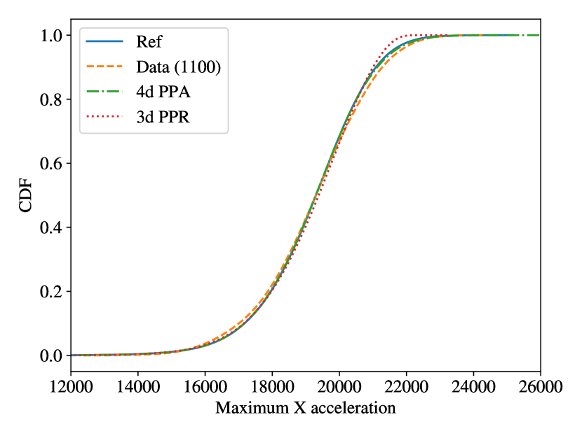
To perform precise analyses, we will choose 1100 MC samples for further analysis. Figures 18 and 18 compare PDFs and CDFs obtained from different models.


We see that the resulting PDF of the PPA method is even closer to the reference than the case of using 700 MC samples. The relative difference between the PPA PDF and the reference PDF has been reduced to 1.9%. The accuracy is improved in all support of the QoI. In addition, the PDF generated directly from the data is different from the reference, especially in the left tail region. Also, comparing the PDF generated from 1100 data in Figure 18 and the PDF generated from 700 data in Figure 16, the data increase only slightly improves the PDF, implying a slow convergence of the MCS. From the CDF figure, the curve associated with the data slightly deviates from the reference, while the result from PPA almost overlaps with the reference.
For this model, we also present the comparison to the PPR model, the additive of univariate PCE models. The same 1100 MC samples are used for PPA and PPR. The results of PDFs and CDFs are shown in Figures 20 and 20.

We see that the PPR model has improved in the left half of the PDF compared to the data. However, it gives unsatisfactory predictions in the right tail regions. The relative error of the PPR model is 11.2% compared to 1.8% of the PPA model. From the CDF comparison, we can also clearly see that the PPR model gives inaccurate reliability information on the right tail.
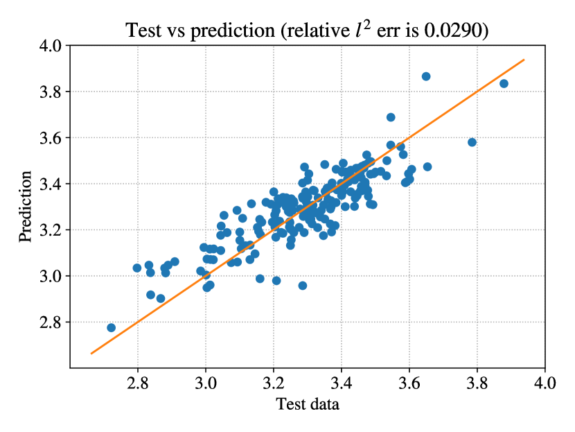
In the case where the PPA model serves as a surrogate model to predict QoI with different input parameters, we generate 200 MC samples that are different from the training data. We can predict the QoI on these 200 samples using the PPA model. The comparison of the prediction and the reference model on the test set is shown in Figure 21.


From the left figure, the PPA prediction is close to the reference on most of the test data. From the right figure, although several data have relatively worse predictions, the scatter dots of prediction against the test set are closely aligned in the unit slope line, meaning that the predictions are close to the reference. The relative difference of the 200 test data is 3.08%, which is close to the relative error of the PPA PDF compared to the reference PDF. The results suggest that the prediction is accurate.
We see that the PPA model has reduced the dimension from 24 to 4 with only 1100 MC samples. The accuracy of the PPA model is comparable to the models proposed by basis adaptation and accelerated basis adaptation methods. The latter two methods adopted the sparse quadrature rule to compute the PCE coefficients and reduce computational costs. Even in that case, the required quadrature points are 2780 and 1757, respectively, which is still greater than 1100. Another observation is that the reduced dimension discovered by PPA is less than that of the basis adaptation methods, which suggests that the low-dimensional manifold found by PPA is better at revealing the probabilistic information of the QoI.
4.2.2 Multi-QoI capability
Another valuable feature of the data-driven essence of PPA is that the data can be reused for different QoIs. One of the limitations of the basis adaptation methods is that each rotation matrix is associated with a scalar QoI. If the QoI is changed, the whole procedure must be repeated to discover a low-dimensional space for the new QoI. This means that new model evaluations are required to compute the PCE coefficients of the newly adapted model. In the PPA, however, the data we are starting from can be reused to train a new model associated with any new QoI. The only additional computation lies in the training process, which is usually much easier, especially when a low-dimensional manifold is discovered. To test its capability, we use the same data and try to train a model for the maximum velocity of the space structure.
In this case, we are not showing the results from basis adaptation and accelerated basis adaptation. However, the accelerated basis adaptation method provides a reference model of the maximum velocity from a 6-dimensional PCE.
Starting from 100 MC samples in the data set, we gradually increase more MC samples. First, a converged PPA model is trained for each data set expressed in PCE. Then, we generate many MC samples based on the PPA model and obtain its PDF by KDE. Finally, the PDFs of the PPA from the data with different samples are compared to the reference PDF. Then, a convergence curve of the relative error can be obtained; see Figure 23.


For the maximum velocity, the PPA model has an error close to 5% when the number of samples in the training data set is 800. Again, in most engineering applications, the accuracy is already enough. The PDF comparison, in this case, is shown in Figure 23. Clearly, the PDF generated by the PPA model is close to the reference with an error of 5.4%, while the PDF generated from the data directly has an error of 19.2%, a large discrepancy from the reference.
To perform precise analyses, we chose 1200 MC samples in the data set (where the PPA model is converged) for further analysis. The PDF and CDF comparisons of different models are shown in Figures 25 and 25.


We see that the PDF obtained from the PPA model is even closer to the reference than when 800 data are used. The relative error has decreased from 5.4% to 2.7%. However, for the PDF obtained from the data, the error barely changes from the 800 data case to the 1200 data case. A significant discrepancy still exists even if the number of samples has increased. This signifies the slow convergence of the traditional MC methods. From Figure 25, we also see that the CDF of the PPA model is consistent with the reference, while the CDF from the data is far from the reference.
Again, we can use the PPA model as a surrogate to predict QoI with different input parameters. For example, we generate 200 MC samples that differ from the training data as the test set. We can predict the QoI on these 200 samples using the PPA model. The comparison of the prediction and the reference model on the test set is shown in Figure 26.

From the left figure, the PPA prediction is close to the reference on most of the test data. This can be seen more evident in the right figure, where the scatter dots of prediction against the test set are closely aligned in the unit slope line, meaning that the predictions are close to the reference. The relative difference of the 200 test data is 2.9%, which is close to the relative error of the PPA PDF compared to the reference PDF. The results suggest that the prediction is accurate.
5 Conclusions
The paper proposed a novel, highly accurate, and efficient surrogate model for high-dimensional computational models and high-dimensional data. Specifically, we proposed a data-driven projection pursuit adaptation method (PPA) that can discover optimal low-dimensional space and polynomial chaos expansions (PCE) to represent the quantity of interest (QoI) accurately. The method has the following significances. First, the dimension reduction capability and optimal PCE representation are based on a-priori-specified data. No additional model evaluations are required. Second, the method can discover even a lower-dimensional localization than other techniques, using even less data. Third, the required data are independent samples, which have less restriction and are relatively easier to obtain than, for example, quadrature points. Lastly, the method has the multi-QoI capability as the same data set can be reused to learn different representations for different QoIs.
The method is developed for uncertainty quantification (UQ) and prediction. In UQ, the basis adaptation method in PCE and its accelerated algorithm present the potential to serve as a general dimension reduction technique. Although versatile, sparse quadrature is often used to construct the PCE models to reduce the computational cost, which requires evaluating the physical model on specific quadrature points. The projection pursuit regression (PPR) model approximates the response for high-dimensional data by a sum of smooth functions of some projected variables. The optimal projections and the smooth functions are found simultaneously from the given data. However, the convergence and capability to represent any variable in the admissible space in PPR depend on the choice of smooth functions. In this paper, we combine the advantages of these two methods and propose the novel PPA method for surrogate modeling of high-dimensional models or data. Specifically, we use multivariate PCE as a smooth function and approximate the response by a multivariate PCE on the projected variables. A stage-wise greedy strategy determines the number of projections, where we simultaneously compute the optimal projection and the optimal multivariate PCE at each stage and stop the procedure if additional information does not improve the approximation significantly. The PPA model inherits the convergence property and the capability to represent any variable in the admissible space from PCE. The applications of a borehole model and a space structure model demonstrate that the PPA model can find low-dimensional spaces to represent the responses accurately. In addition, the number of samples required to obtain accurate results in PPA is even less than the accelerated basis adaptation, where the latter uses sparse quadrature points. The space structure example also shows that the method can be applied to multiple QoIs using the same data set.
Acknowledgments
We acknowledge support through ONR Grant No. N00014-21-1-2475 with Dr. Eric Marineau as Program Manager. Financial support is also acknowledged by the United States Department of Energy through Framework, Algorithms, and Scalable Technologies for Mathematics (FASTMATH) SciDac Institute under Grant No. DE-SC0021307 with Dr. Ceren Susut ad Program Manager.
References
- Ghanem and Spanos [1991] R. Ghanem, P. D. Spanos, Stochastic Finite Elements: A Spectral Approach, Springer-Verlag, 1991.
- Ghanem and Red-Horse [1999] R. Ghanem, J. Red-Horse, Propagation of probabilistic uncertainty in complex physical systems using a stochastic finite element approach, Physica D: Nonlinear Phenomena 133 (1999) 137–144.
- Sudret [2007] B. Sudret, Uncertainty propagation and sensitivity analysis in mechanical models–contributions to structural reliability and stochastic spectral methods, Habilitationa diriger des recherches, Université Blaise Pascal, Clermont-Ferrand, France 147 (2007) 53.
- Najm [2009] H. N. Najm, Uncertainty quantification and polynomial chaos techniques in computational fluid dynamics, Annual review of fluid mechanics 41 (2009) 35–52.
- Soize [2017] C. Soize, Uncertainty quantification, Springer, 2017.
- Chen et al. [2017] J. Chen, X. Zeng, Y. Peng, Probabilistic analysis of wind-induced vibration mitigation of structures by fluid viscous dampers, Joural of Sound and Vibration 409 (2017) 287–305.
- Zeng et al. [2017] X. Zeng, Y. Peng, J. Chen, Serviceability-based damping optimization of randomly wind-excited high-rise buildings, The structural design of tall and special buildings 26 (2017) e1371.
- Marzouk et al. [2007] Y. M. Marzouk, H. N. Najm, L. A. Rahn, Stochastic spectral methods for efficient Bayesian solution of inverse problems, Journal of Computational Physics 224 (2007) 560–586.
- Marzouk and Najm [2009] Y. M. Marzouk, H. N. Najm, Dimensionality reduction and polynomial chaos acceleration of Bayesian inference in inverse problems, Journal of Computational Physics 228 (2009) 1862–1902.
- Marzouk and Xiu [2009] Y. Marzouk, D. Xiu, A stochastic collocation approach to Bayesian inference in inverse problems (2009).
- Sudret et al. [2017] B. Sudret, S. Marelli, J. Wiart, Surrogate models for uncertainty quantification: An overview, in: 2017 11th European conference on antennas and propagation (EUCAP), IEEE, 2017, pp. 793–797.
- Ghanem [1999] R. Ghanem, Ingredients for a general purpose stochastic finite elements implementation, Computer Methods in Applied Mechanics and Engineering 168 (1999) 19–34.
- Xiu and Karniadakis [2002a] D. Xiu, G. E. Karniadakis, The Wiener–Askey polynomial chaos for stochastic differential equations, SIAM journal on scientific computing 24 (2002a) 619–644.
- Xiu and Karniadakis [2002b] D. Xiu, G. E. Karniadakis, Modeling uncertainty in steady state diffusion problems via generalized polynomial chaos, Computer methods in applied mechanics and engineering 191 (2002b) 4927–4948.
- MacKay et al. [1998] D. J. MacKay, et al., Introduction to gaussian processes, NATO ASI series F computer and systems sciences 168 (1998) 133–166.
- Seeger [2004] M. Seeger, Gaussian processes for machine learning, International journal of neural systems 14 (2004) 69–106.
- Bilionis and Zabaras [2012] I. Bilionis, N. Zabaras, Multi-output local gaussian process regression: Applications to uncertainty quantification, Journal of Computational Physics 231 (2012) 5718–5746.
- Li and Chen [2009] J. Li, J. Chen, Stochastic Dynamics of Structures, John Wiley & Sons, 2009.
- Chen et al. [2016] J. Chen, J. Yang, J. Li, A GF-discrepancy for point selection in stochastic seismic response analysis of structures with uncertain parameters, Structural Safety 59 (2016) 20–31.
- Soize and Ghanem [2021] C. Soize, R. Ghanem, Probabilistic learning on manifolds constrained by nonlinear partial differential equations for small datasets, Computer Methods in Applied Mechanics and Engineering 380 (2021) 113777.
- Zhang et al. [2021] H. Zhang, J. Guilleminot, L. J. Gomez, Stochastic modeling of geometrical uncertainties on complex domains, with application to additive manufacturing and brain interface geometries, Computer Methods in Applied Mechanics and Engineering 385 (2021) 114014.
- Giovanis and Shields [2020] D. G. Giovanis, M. D. Shields, Data-driven surrogates for high dimensional models using gaussian process regression on the grassmann manifold, Computer Methods in Applied Mechanics and Engineering 370 (2020) 113269.
- Kougioumtzoglou and Spanos [2012] I. Kougioumtzoglou, P. Spanos, An analytical wiener path integral technique for non-stationary response determination of nonlinear oscillators, Probabilistic Engineering Mechanics 28 (2012) 125–131.
- Psaros et al. [2019] A. F. Psaros, I. Petromichelakis, I. A. Kougioumtzoglou, Wiener path integrals and multi-dimensional global bases for non-stationary stochastic response determination of structural systems, Mechanical Systems and Signal Processing 128 (2019) 551–571.
- Babuška et al. [2007] I. Babuška, F. Nobile, R. Tempone, A stochastic collocation method for elliptic partial differential equations with random input data, SIAM Journal on Numerical Analysis 45 (2007) 1005–1034.
- Le Maitre and Knio [2010] O. Le Maitre, O. M. Knio, Spectral methods for uncertainty quantification: with applications to computational fluid dynamics, Springer Science & Business Media, 2010.
- Smolyak [1963] S. A. Smolyak, Quadrature and interpolation formulas for tensor products of certain classes of functions, Doklady Akademii Nauk 4 (1963) 240–243.
- Gerstner and Griebel [1998] T. Gerstner, M. Griebel, Numerical integration using sparse grids, Numerical algorithms 18 (1998) 209–232.
- Novak and Ritter [1999] E. Novak, K. Ritter, Simple cubature formulas with high polynomial exactness, Constructive approximation 15 (1999) 499–522.
- Blatman and Sudret [2010] G. Blatman, B. Sudret, An adaptive algorithm to build up sparse polynomial chaos expansions for stochastic finite element analysis, Probabilistic Engineering Mechanics 25 (2010) 183–197.
- Blatman and Sudret [2011] G. Blatman, B. Sudret, Adaptive sparse polynomial chaos expansion based on least angle regression, Journal of Computational Physics 230 (2011) 2345–2367.
- Doostan and Owhadi [2011] A. Doostan, H. Owhadi, A non-adapted sparse approximation of PDEs with stochastic inputs, Journal of Computational Physics 230 (2011) 3015–3034.
- Sargsyan et al. [2014] K. Sargsyan, C. Safta, H. N. Najm, B. J. Debusschere, D. Ricciuto, P. Thornton, Dimensionality reduction for complex models via Bayesian compressive sensing, International Journal for Uncertainty Quantification 4 (2014) 63–93.
- Hampton and Doostan [2015] J. Hampton, A. Doostan, Compressive sampling of polynomial chaos expansions: Convergence analysis and sampling strategies, Journal of Computational Physics 280 (2015) 363–386.
- Constantine et al. [2014] P. G. Constantine, E. Dow, Q. Wang, Active subspace methods in theory and practice: applications to kriging surfaces, SIAM Journal on Scientific Computing 36 (2014) A1500–A1524.
- Constantine [2015] P. G. Constantine, Active Subspaces: Emerging Ideas for Dimension Reduction in Parameter Studies, volume 2, SIAM, 2015.
- Tipireddy and Ghanem [2014] R. Tipireddy, R. Ghanem, Basis adaptation in homogeneous chaos spaces, Journal of Computational Physics 259 (2014) 304–317.
- Thimmisetty et al. [2017] C. Thimmisetty, P. Tsilifis, R. Ghanem, Homogeneous chaos basis adaptation for design optimization under uncertainty: Application to the oil well placement problem, Ai Edam 31 (2017) 265–276.
- Ghauch et al. [2019] Z. G. Ghauch, V. Aitharaju, W. R. Rodgers, P. Pasupuleti, A. Dereims, R. G. Ghanem, Integrated stochastic analysis of fiber composites manufacturing using adapted polynomial chaos expansions, Composites Part A: Applied Science and Manufacturing 118 (2019) 179–193.
- Zeng et al. [2021] X. Zeng, J. Red-Horse, R. Ghanem, Accelerated basis adaptation in homogeneous chaos spaces, Computer Methods in Applied Mechanics and Engineering 386 (2021) 114109.
- Cai et al. [2018] J. Cai, J. Luo, S. Wang, S. Yang, Feature selection in machine learning: A new perspective, Neurocomputing 300 (2018) 70–79.
- Murphy [2012] K. P. Murphy, Machine learning: a probabilistic perspective, MIT press, 2012.
- Howley et al. [2005] T. Howley, M. G. Madden, M.-L. O’Connell, A. G. Ryder, The effect of principal component analysis on machine learning accuracy with high dimensional spectral data, in: International Conference on Innovative Techniques and Applications of Artificial Intelligence, Springer, 2005, pp. 209–222.
- Reddy et al. [2020] G. T. Reddy, M. P. K. Reddy, K. Lakshmanna, R. Kaluri, D. S. Rajput, G. Srivastava, T. Baker, Analysis of dimensionality reduction techniques on big data, IEEE Access 8 (2020) 54776–54788.
- McInnes et al. [2018] L. McInnes, J. Healy, J. Melville, Umap: Uniform manifold approximation and projection for dimension reduction, arXiv preprint arXiv:1802.03426 (2018).
- Lin and Zha [2008] T. Lin, H. Zha, Riemannian manifold learning, IEEE Transactions on Pattern Analysis and Machine Intelligence 30 (2008) 796–809.
- Han et al. [2018] K. Han, Y. Wang, C. Zhang, C. Li, C. Xu, Autoencoder inspired unsupervised feature selection, in: 2018 IEEE international conference on acoustics, speech and signal processing (ICASSP), IEEE, 2018, pp. 2941–2945.
- Baldi [2012] P. Baldi, Autoencoders, unsupervised learning, and deep architectures, in: Proceedings of ICML workshop on unsupervised and transfer learning, JMLR Workshop and Conference Proceedings, 2012, pp. 37–49.
- Friedman and Tukey [1974] J. H. Friedman, J. W. Tukey, A projection pursuit algorithm for exploratory data analysis, IEEE Transactions on computers 100 (1974) 881–890.
- Huber [1985] P. J. Huber, Projection pursuit, The annals of Statistics (1985) 435–475.
- Friedman [1987] J. H. Friedman, Exploratory projection pursuit, Journal of the American statistical association 82 (1987) 249–266.
- Lee et al. [2005] E.-K. Lee, D. Cook, S. Klinke, T. Lumley, Projection pursuit for exploratory supervised classification, Journal of Computational and graphical Statistics 14 (2005) 831–846.
- Grochowski and Duch [2008] M. Grochowski, W. Duch, Projection pursuit constructive neural networks based on quality of projected clusters, in: International Conference on Artificial Neural Networks, Springer, 2008, pp. 754–762.
- Barcaru [2019] A. Barcaru, Supervised projection pursuit–a dimensionality reduction technique optimized for probabilistic classification, Chemometrics and Intelligent Laboratory Systems 194 (2019) 103867.
- Grear et al. [2021] T. Grear, C. Avery, J. Patterson, D. J. Jacobs, Molecular function recognition by supervised projection pursuit machine learning, Scientific reports 11 (2021) 1–15.
- Olivier et al. [2021] A. Olivier, M. D. Shields, L. Graham-Brady, Bayesian neural networks for uncertainty quantification in data-driven materials modeling, Computer Methods in Applied Mechanics and Engineering 386 (2021) 114079.
- Yang et al. [2021] L. Yang, X. Meng, G. E. Karniadakis, B-pinns: Bayesian physics-informed neural networks for forward and inverse pde problems with noisy data, Journal of Computational Physics 425 (2021) 109913.
- Leibig et al. [2017] C. Leibig, V. Allken, M. S. Ayhan, P. Berens, S. Wahl, Leveraging uncertainty information from deep neural networks for disease detection, Scientific reports 7 (2017) 1–14.
- Friedman and Stuetzle [1981] J. H. Friedman, W. Stuetzle, Projection pursuit regression, Journal of the American statistical Association 76 (1981) 817–823.
- Hastie et al. [2009] T. Hastie, R. Tibshirani, J. H. Friedman, J. H. Friedman, The elements of statistical learning: data mining, inference, and prediction, volume 2, Springer, 2009.
- Qianjian and Jianguo [2011] G. Qianjian, Y. Jianguo, Application of projection pursuit regression to thermal error modeling of a cnc machine tool, The International Journal of Advanced Manufacturing Technology 55 (2011) 623–629.
- Ferraty et al. [2013] F. Ferraty, A. Goia, E. Salinelli, P. Vieu, Functional projection pursuit regression, Test 22 (2013) 293–320.
- Durocher et al. [2015] M. Durocher, F. Chebana, T. B. Ouarda, A nonlinear approach to regional flood frequency analysis using projection pursuit regression, Journal of Hydrometeorology 16 (2015) 1561–1574.
- Cui et al. [2017] H.-Y. Cui, Y. Zhao, Y.-N. Chen, X. Zhang, X.-Q. Wang, Q. Lu, L.-M. Jia, Z.-M. Wei, Assessment of phytotoxicity grade during composting based on eem/parafac combined with projection pursuit regression, Journal of hazardous materials 326 (2017) 10–17.
- Janson et al. [1997] S. Janson, et al., Gaussian Hilbert Spaces, Cambridge University Press, 1997.
- Cohen and Migliorati [2017] A. Cohen, G. Migliorati, Optimal weighted least-squares methods, The SMAI journal of computational mathematics 3 (2017) 181–203.
- Schwab and Gittelson [2011] C. Schwab, C. J. Gittelson, Sparse tensor discretizations of high-dimensional parametric and stochastic PDEs, Acta Numerica 20 (2011) 291–467.
- Rosenblatt [1952] M. Rosenblatt, Remarks on a multivariate transformation, The annals of mathematical statistics 23 (1952) 470–472.
- Tsilifis and Ghanem [2017] P. Tsilifis, R. G. Ghanem, Reduced Wiener chaos representation of random fields via basis adaptation and projection, Journal of Computational Physics 341 (2017) 102–120.