This paper was converted on www.awesomepapers.org from LaTeX by an anonymous user.
Want to know more? Visit the Converter page.

Projection based adiabatic elimination of bipartite open quantum systems

Ibrahim Saideh Laboratoire Matériaux et Phénomènes Quantiques, Université Paris Diderot, CNRS UMR 7162, 75013, Paris, France. Université Paris-Saclay, 91405 Orsay, France    Daniel Finkelstein-Shapiro Division of Chemical Physics, Lund University, Box 124, 221 00 Lund, Sweden    Camille Noûs Cogitamus Laboratory [email protected]    Tõnu Pullerits Division of Chemical Physics, Lund University, Box 124, 221 00 Lund, Sweden    Arne Keller Laboratoire Matériaux et Phénomènes Quantiques, Université Paris Diderot, CNRS UMR 7162, 75013, Paris, France. Université Paris-Saclay, 91405 Orsay, France [email protected]
Abstract

Adiabatic elimination methods allow the reduction of the space dimension needed to describe systems dynamics which exhibits separation of time scale. For open quantum system, it consists in eliminating the fast part assuming it has almost instantaneously reached its steady-state and obtaining an approximation of the evolution of the slow part. These methods can be applied to eliminate a linear subspace within the system Hilbert space, or alternatively to eliminate a fast subsystems in a bipartite quantum system. In this work, we extend an adiabatic elimination method used for removing fast degrees of freedom within a open quantum system (Phys. Rev. A 2020, 101, 042102) to eliminate a subsystem from an open bipartite quantum system. As an illustration, we apply our technique to a dispersively coupled two-qubit system and in the case of the open Rabi model.

I Introduction

Adiabatic elimination is a method whereby the fast degrees of freedom of a system are removed while retaining an effective description of the slow degrees of freedom. This simplification can be very useful to obtain tractable and intuitive equations when only a coarse-grained or long times description is desired Haken (1975, 1977); Lax (1967); Cohen-Tannoudji (1992); Paulisch et al. (2014); Brion et al. (2007); You et al. (2003); Nagy et al. (2010); Douglas et al. (2015), depending on if the target system has a conservative Paulisch et al. (2014); Sinatra et al. (1995); Brion et al. (2007) or a dissipative Azouit et al. (2016, 2017a); Azouit (2017); Azouit et al. (2017b); Sarlette et al. (2020); Mirrahimi and Rouchon (2009); Reiter and Sørensen (2012); Kessler (2012) evolution. There are two classes of manifolds on which adiabatic elimination has been applied, i) those that consist of levels within a subsystem, for example the excited states of an atom, and ii) those that consist of a separate subsystem, such as ancillary qubits or measuring devices. For a slow and fast parts described by Hilbert spaces (A)\mathcal{H}^{(A)} and (B)\mathcal{H}^{(B)}, the first case corresponds to the Hilbert space =(A)(B)\mathcal{H}=\mathcal{H}^{(A)}\oplus\mathcal{H}^{(B)} (direct sum) while the second case corresponds to the Hilbert space =(A)(B)\mathcal{H}=\mathcal{H}^{(A)}\otimes\mathcal{H}^{(B)} (tensor product). Adiabatic elimination is useful in developing protocols for dissipative state preparation in ion traps Lin et al. (2013); Albert et al. (2019), reservoir engineering Pastawski et al. (2011) and the description of measurement devices Černotík et al. (2015). The simplicity of the resulting equations can also be computationally advantageous in the study of quantum phase transitions where the size of the system is cumbersomly large Minganti et al. (2018).

There are several approaches to obtain effective operators, ranging from perturbative expansions of the Liouville operator Reiter and Sørensen (2012); Kessler (2012), the corresponding Kraus maps Mirrahimi and Rouchon (2009); Azouit et al. (2016, 2017a, 2017b); Azouit (2017), the resolvent Finkelstein-Shapiro et al. (2020), or using stochastic methods Černotík et al. (2015). Eliminating a fast subsystem (that forms a tensor product with the slow subsystem) is typically done with a partial trace over the fast subsystem. This can result in a set of hierarchical equations that allows error estimation and correcting the approximation as the slow and fast timescales get closer. Importantly, the expansion can be built to preserve the Lindblad structure and as a consequence the physicality of the map Azouit et al. (2017a); Lesanovsky and Garrahan (2013); Marcuzzi et al. (2014). The procedure for eliminating sublevels within a subsystem (direct sum with the slow subsystem) is best carried out with Feshbach projections Reiter and Sørensen (2012); Finkelstein-Shapiro et al. (2020). However, as the fast-slow separation breaks down, or when incoherent pumping channels exist, the population of the fast subsystem becomes non-negligible (i.e. there can be a finite fraction of population in the excited states). When this happens, the exact time evolution of the slow part becomes non-trace preserving. The loss of trace can be corrected using contour integral methods Finkelstein-Shapiro et al. (2020). It would be however advantageous to have a method that can handle both classes of fast manifolds. This is more important considering that systems from atomic physics are inspiring a number of chemical versions that have much more complicated Hamiltonians and it would be ideal to transform them into effective operators for a direct comparison to the atomic physics counterparts Castellini et al. (2018); Finkelstein-Shapiro et al. ; Ribeiro et al. (2018).

In this work, we extend the methodology developed in Ref. Finkelstein-Shapiro et al. (2020) to bipartite open quantum systems whose dynamics are described by a Lindblad operator Lindblad (1976); Gorini et al. (1976). We use the projection operator method suggested by Knezevic and Berry Knezevic and Ferry (2002) in order to derive equations for a slow subsystem AA coupled to a fast subsystem BB. The paper is organized as follows. We first recall the main results of Ref Finkelstein-Shapiro et al. (2020). We then apply it to the general bipartite case to obtain a recipe for describing the slow subsystem. Finally, we illustrate the method in the case of a spin dispersively coupled to a second highly dissipative driven spin and to describe the dynamics of the open Rabi model.

II Theory

II.1 Adiabatic elimination through projectors techniques

Let ρ(t)\rho(t) be the density operator on the Hilbert space \mathcal{H} describing the quantum state of the system at time tt. We suppose that the evolution of ρ(t)\rho(t) is generated by a Lindblad operator \mathcal{L}: ρ˙(t)=ρ(t)\dot{\rho}(t)=\mathcal{L}\rho(t). We define the Hilbert space \mathbfcal{H} of operator OO on \mathcal{H}, equipped with the scalar product tr[O1O2]\text{tr}\left[O_{1}^{\dagger}O_{2}\right]. We first recall the main results presented in Ref Finkelstein-Shapiro et al. (2020) related to projector techniques. Let 𝒫\mathcal{P} the projector such that ρs(t)=𝒫ρ(t)\rho_{s}(t)=\mathcal{P}\rho(t) is the the slow part of the system and write 𝒬=𝟙𝒫\mathcal{Q}=\openone-\mathcal{P}, where 𝟙\openone is the identity operator on \mathbfcal{H}. Let 𝒢(z)=(z)1\mathcal{G}(z)=(z-\mathcal{L})^{-1} be the resolvent of the Lindblad operator \mathcal{L}. Operators like 𝒫,𝒬,\mathcal{P},\mathcal{Q},\mathcal{L} or 𝒢\mathcal{G} are operators on \mathbfcal{H}. They are sometimes called super-operators. They are here denoted with calligraphic letter, to distinguish them from operators on \mathcal{H} (belonging to \mathbfcal{H}), like the density matrix ρ\rho.

We define the effective Lindblad operator eff(z)\mathcal{L}_{\text{eff}}(z), such that 𝒫𝒢(z)𝒫=(zeff(z))1\mathcal{P}\mathcal{G}(z)\mathcal{P}=(z-\mathcal{L}_{\text{eff}}(z))^{-1}. The effective Lindblad operator eff(z)\mathcal{L}_{\text{eff}}(z) can be written as :

eff(z)=𝒫𝒫+𝒫𝒬𝒢0(z)𝒬𝒫,\mathcal{L}_{\text{eff}}(z)=\mathcal{P}\mathcal{L}\mathcal{P}+\mathcal{P}\mathcal{L}\mathcal{Q}\mathcal{G}_{0}(z)\mathcal{Q}\mathcal{L}\mathcal{P}, (1)

where

𝒬𝒢0(z)𝒬=(z𝒬𝒬)1.\mathcal{Q}\mathcal{G}_{0}(z)\mathcal{Q}=(z-\mathcal{Q}\mathcal{L}\mathcal{Q})^{-1}. (2)

For any ρ(t=0)\rho(t=0), such that 𝒬ρ(t=0)=0\mathcal{Q}\rho(t=0)=0, the slow dynamics inside 𝒫\mathcal{P}\mathbfcal{H} can be obtained with the inverse Laplace transform as:

ρs(t)=12πiDdzezt𝒫G(z)𝒫ρs(t=0),\rho_{s}(t)=\frac{1}{2\pi i}\int_{D}\mathrm{d}ze^{zt}\mathcal{P}G(z)\mathcal{P}\rho_{s}(t=0), (3)

where ρs(t=0)=𝒫ρ(t=0)\rho_{s}(t=0)=\mathcal{P}\rho(t=0) and the integral on the complex plane is performed on a straight line D={z;z=a>0}D=\left\{z\in\mathbb{C};\Re{z}=a>0\right\}. At this point no approximation has been made. Eq. (3) gives the exact dynamics inside 𝒫\mathcal{P}\mathbfcal{H}, as long as the initial condition is also inside 𝒫\mathcal{P}\mathbfcal{H}, that is 𝒬ρ(t=0)=0\mathcal{Q}\rho(t=0)=0. Because eff(z)\mathcal{L}_{\text{eff}}(z) captures the effect of the dynamics in 𝒬\mathcal{Q}\mathbfcal{H}, it is a nonlinear superoperator, in the sense that (zeff(z))ν=0(z-\mathcal{L}_{\text{eff}}(z))\vec{\nu}=0 is a nonlinear eigenvalue problem.

The approximation of a slow dynamics of 𝒫ρ(t)\mathcal{P}\rho(t), with respect to the fast dynamics of 𝒬ρ(t)\mathcal{Q}\rho(t) is equivalent to considering the dynamics inside 𝒫\mathcal{P}\mathbfcal{H} in the vicinity of the stationary state reached in the limit tt\rightarrow\infty. In this long time limit only the z0z\rightarrow 0 limit will contribute to the inverse Laplace transform of Eq. (3). We thus approximate eff(z)\mathcal{L}_{\text{eff}}(z) to the lowest relevant order:

eff(z)0+z1++znn\mathcal{L}_{\text{eff}}(z)\simeq\mathcal{L}_{0}+z\mathcal{L}_{1}+\cdots+z^{n}\mathcal{L}_{n} (4)

where 0=eff(z=0)\mathcal{L}_{0}=\mathcal{L}_{\text{eff}}(z=0) and n=1n!ddzeff(z)|z=0\mathcal{L}_{n}=\frac{1}{n!}\left.\frac{\mathrm{d}}{\mathrm{d}z}\mathcal{L}_{\text{eff}}(z)\right|_{z=0}. Using the expression of eff(z)\mathcal{L}_{\text{eff}}(z) given by Eq. (1) allows to express 0\mathcal{L}_{0} and n\mathcal{L}_{n} as:

0\displaystyle\mathcal{L}_{0} =𝒫𝒫𝒫𝒬(𝒬𝒬)1𝒬𝒫\displaystyle=\mathcal{P}\mathcal{L}\mathcal{P}-\mathcal{P}\mathcal{L}\mathcal{Q}(\mathcal{Q}\mathcal{L}\mathcal{Q})^{-1}\mathcal{Q}\mathcal{L}\mathcal{P}
n\displaystyle\mathcal{L}_{n} =𝒫𝒬(𝒬𝒬)(n+1)𝒬𝒫.\displaystyle=-\mathcal{P}\mathcal{L}\mathcal{Q}\left(\mathcal{Q}\mathcal{L}\mathcal{Q}\right)^{-(n+1)}\mathcal{Q}\mathcal{L}\mathcal{P}. (5)

In this work, we consider the approximation given by Eq. (4) with n1n\leq 1 only, which is a standard approximation for most of the effective operators that are calculated explicitly. The systematic study of higher order approximations (n>1n>1) will be considered in a future work. Within the approximation given by Eq. (4), with n=1n=1, the inverse Laplace transform of Eq. (3) can be computed explicitly. We obtain:

ρs(t)=exp[(11)10t](11)1ρs(t=0)\rho_{s}(t)=\exp\left[(1-\mathcal{L}_{1})^{-1}\mathcal{L}_{0}t\right](1-\mathcal{L}_{1})^{-1}\rho_{s}(t=0) (6)

The stationary state ρf\rho_{f} of this dynamics, reached at t+t\rightarrow+\infty, is in the kernel of 0\mathcal{L}_{0}. We note that although the dynamics described by Eq. (6) is an approximation, the final reached stationary state ρf\rho_{f} is the exact one.

To conclude, after the adiabatic elimination of the fast part, the generator of the slow dynamics is approximatively given by (11)10(1-\mathcal{L}_{1})^{-1}\mathcal{L}_{0}, ρ˙(t)=(11)10ρ(t)\dot{\rho}(t)=(1-\mathcal{L}_{1})^{-1}\mathcal{L}_{0}\rho(t), where 0\mathcal{L}_{0} and 1\mathcal{L}_{1} can in principle be computed using Eq. (5). The hard part in these equations is the evaluation of the inverse (𝒬𝒬)1(\mathcal{Q}\mathcal{L}\mathcal{Q})^{-1}, which in the most general case, as we will see later, can only be achieved through a perturbative expansion.

Theses results are very general, and require only the definition of a projector 𝒫\mathcal{P} and that the initial state fulfills the condition 𝒬ρ(t=0)=0\mathcal{Q}\rho(t=0)=0. We note that 𝒫\mathcal{P} doesn’t have to be hermitian, that is the projection does not need to be orthogonal.

In Ref. Finkelstein-Shapiro et al. (2020), this formalism was applied to the case where the slow and fast degrees of freedom correspond to a partition of the underlying Hilbert space in two complementary sub-spaces, that is =(A)(B)\mathcal{H}=\mathcal{H}^{(A)}\oplus\mathcal{H}^{(B)}. In the next section we will adapt this general formalism to the bipartite case where =(A)(B)\mathcal{H}=\mathcal{H}^{(A)}\otimes\mathcal{H}^{(B)}.

II.2 Adiabatic elimination in a bipartite system

We suppose that the state of the bipartite system at time tt is described by a density operator ρ(AB)(t)\rho^{(AB)}(t) acting on the Hilbert space =(A)(B)\mathcal{H}=\mathcal{H}^{(A)}\otimes\mathcal{H}^{(B)}. We consider that the dynamics of subsystem AA is very slow compared to the dynamics of subsystem BB. We suppose that the exact stationary state in \mathbfcal{H} is unique and that it is a product state ρf=ρaρb\rho_{f}=\rho_{a}\otimes\rho_{b}, where ρa𝒜\rho_{a}\in\mathbfcal{H}^{(A)} and ρb\rho_{b}\in\mathbfcal{H}^{(B)} with 𝒜\mathbfcal{H}^{(i)},i=A,B, the Hilbert space of operators on (i)\mathcal{H}^{(i)}. As the the dynamics of BB subsystem is very fast, we suppose that it is a good approximation to consider that at t=0t=0, ρ(AB)(t=0)=ρ0(A)ρb\rho^{(AB)}(t=0)=\rho^{(A)}_{0}\otimes\rho_{b}. In other word, we consider that BB reaches its steady state instantaneously in the time scale of the subsystem AA. We thus define 𝒫\mathcal{P} as

𝒫ρ(AB)(t)=trB[ρ(AB)(t)]ρb,\mathcal{P}\rho^{(AB)}(t)=\text{tr}_{B}\left[\rho^{(AB)}(t)\right]\otimes\rho_{b}, (7)

where trB[]\text{tr}_{B}\left[\right] denotes the partial trace over BB. The reduced density operator ρ(A)(t)\rho^{(A)}(t) in 𝒜\mathbfcal{H}^{(A)} can then be obtained as ρ(A)(t)=trB[𝒫ρ(AB)(t)]\rho^{(A)}(t)=\text{tr}_{B}\left[\mathcal{P}\rho^{(AB)}(t)\right].

For the purpose of simplifying some expressions and calculations, it will be useful to use the operator-vector isomorphism Havel (2003) which maps each element of \mathbfcal{H} to a vector in \mathcal{H}\otimes\mathcal{H} as follows. An operators such as |ab|\lvert a\rangle\langle b\rvert\in\mathbfcal{H} is mapped to the vector |b¯|a\lvert\overline{b}\rangle\otimes\lvert a\rangle in the \mathcal{H}\otimes\mathcal{H} Hilbert space, where |b¯\lvert\overline{b}\rangle is the complex conjugate of |b\lvert b\rangle. Consequently, any n×nn\times n density matrix ρ\rho\in\mathbfcal{H} is mapped to a column vector ||ρ\lvert\lvert\rho\rangle\rangle\in\mathcal{H}\otimes\mathcal{H}, with n2n^{2} elements, by stacking the columns of the ρ\rho matrix. Under this isomorphism, super-operators on \mathbfcal{H} are mapped to operators on \mathcal{H}\otimes\mathcal{H}. In particular, the super-operator 𝒪\mathcal{O} performing the operation ρO1ρO2\rho\rightarrow O_{1}\rho O_{2}^{\dagger}, with O1O_{1} and O2O_{2} operators in \mathbfcal{H}, is mapped to ||ρO¯2O1||ρ\lvert\lvert\rho\rangle\rangle\rightarrow\overline{O}_{2}\otimes O_{1}\lvert\lvert\rho\rangle\rangle, where O¯\overline{O} denotes the complex conjugate of OO; that is O¯=(O)T\overline{O}=\left(O^{\dagger}\right)^{T}, where OO^{\dagger} is the adjoint and OTO^{T} is the transpose of OO. In this way, the scalar product tr[ρ1ρ2]\text{tr}\left[\rho_{1}^{\dagger}\rho_{2}\right] between two operators ρ1\rho_{1} and ρ2\rho_{2} in \mathbfcal{H} is equal to the usual scalar product ρ1|ρ2\langle\langle\rho_{1}\rvert\rho_{2}\rangle\rangle in \mathcal{H}\otimes\mathcal{H}. Some useful remarks can be made. The identity operator 𝟙\openone in \mathbfcal{H} is mapped to the maximally entangled state

||𝟙=𝕜|𝕜|𝕜\lvert\lvert\openone\rangle\rangle=\sum_{k}\lvert k\rangle\otimes\lvert k\rangle (8)

in \mathcal{H}\otimes\mathcal{H}, where {|k}\left\{\lvert k\rangle\right\} is an orthonormal basis of \mathcal{H}. We also note that the usual density matrix normalization tr[ρ]=1\text{tr}\left[\rho\right]=1 does not correspond to the normalization induced by the scalar product tr[ρ2]=1\text{tr}\left[\rho^{2}\right]=1 (except in the case of a pure state). Using the previous remark, we have that tr[ρ]=tr[𝟙ρ]=1\text{tr}\left[\rho\right]=\text{tr}\left[\openone\rho\right]=1 is mapped to 𝟙|ρ=𝟙\langle\langle\openone\rvert\rho\rangle\rangle=1. For our bipartite case, =(A)(B)\mathcal{H}=\mathcal{H}^{(A)}\otimes\mathcal{H}^{(B)}. Therefore, an operator in \mathbfcal{H} as |a1a2||b1b2|\lvert a_{1}\rangle\langle a_{2}\rvert\otimes\lvert b_{1}\rangle\langle b_{2}\rvert, where |ai(bi)(A)((B))(i=1,2)\lvert a_{i}(b_{i})\rangle\in\mathcal{H}^{(A)}(\mathcal{H}^{(B)})(i=1,2), is mapped to |a2¯|a1|b2¯|b1\lvert\overline{a_{2}}\rangle\otimes\lvert a_{1}\rangle\otimes\lvert\overline{b_{2}}\rangle\otimes\lvert b_{1}\rangle. The partial trace over (B)\mathcal{H}^{(B)}, trB[ρ]𝒜\text{tr}_{B}\left[\rho\right]\in\mathbfcal{H}^{(A)} is mapped to 𝟙(𝔹)|ρ(𝔸)(𝔸)\langle\langle\openone^{(B)}\rvert\rho\rangle\rangle\in\mathcal{H}^{(A)}\otimes\mathcal{H}^{(A)}, where |𝟙(𝔹)=𝕜|𝕜|𝕜\lvert\openone^{(B)}\rangle=\sum_{k}\lvert k\rangle\otimes\lvert k\rangle in (B)(B)\mathcal{H}^{(B)}\otimes\mathcal{H}^{(B)}, where {|k}\left\{\lvert k\rangle\right\} is now an orthonormal basis of (B)\mathcal{H}^{(B)}.

Consequently, the operator 𝒫ρ(AB)\mathcal{P}\rho^{(AB)}\in\mathbfcal{H} is mapped to the vector 𝟙(𝔹)|ρ(𝔸𝔹)||ρ𝕓\langle\langle\openone^{(B)}\rvert\rho^{(AB)}\rangle\rangle\otimes\lvert\lvert\rho_{b}\rangle\rangle\in\mathcal{H}\otimes\mathcal{H}. The projector 𝒫\mathcal{P} acting on \mathcal{H}\otimes\mathcal{H} can thus be written as:

𝒫=𝟙(𝟚𝔸)𝒫(𝟚𝔹) with 𝒫(𝟚𝔹)=||ρ𝕓𝟙(𝔹)||\mathcal{P}=\openone^{(2A)}\otimes\mathcal{P}^{(2B)}\text{ with }\mathcal{P}^{(2B)}=\lvert\lvert\rho_{b}\rangle\rangle\langle\langle\openone^{(B)}\rvert\rvert (9)

where 𝟙(𝟚𝔸)\openone^{(2A)} is the identity operator on (A)(A)\mathcal{H}^{(A)}\otimes\mathcal{H}^{(A)}. The operator 𝒬=𝟙𝒫\mathcal{Q}=\openone-\mathcal{P} simply reads as:

𝒬=𝟙(𝟚𝔸)𝒬(𝟚𝔹) with 𝒬(𝟚𝔹)=𝟙(𝟚𝔹)𝒫(𝟚𝔹),\mathcal{Q}=\openone^{(2A)}\otimes\mathcal{Q}^{(2B)}\text{ with }\mathcal{Q}^{(2B)}=\openone^{(2B)}-\mathcal{P}^{(2B)}, (10)

where 𝟙(𝟚𝔹)\openone^{(2B)} is the identity operator on (B)(B)\mathcal{H}^{(B)}\otimes\mathcal{H}^{(B)}.

In general, the Lindblad operator of the system can be split in 3 terms as follows:

=A𝟙(𝟚𝔹)+𝟙(𝟚𝔸)𝔹+𝔸𝔹\mathcal{L}=\mathcal{L}_{A}\otimes\openone^{(2B)}+\openone^{(2A)}\otimes\mathcal{L}_{B}+\mathcal{L}_{AB} (11)

where A(B)\mathcal{L}_{A(B)} is a Lindblad operator acting on the A(B)A(B) part only. The decomposition of \mathcal{L} with the help of 𝒫\mathcal{P} and 𝒬\mathcal{Q} reads:

𝒫𝒫\displaystyle\mathcal{P}\mathcal{L}\mathcal{P} =A𝒫B+𝒫AB𝒫\displaystyle=\mathcal{L}_{A}\otimes\mathcal{P}_{B}+\mathcal{P}\mathcal{L}_{AB}\mathcal{P} (12)
𝒫𝒬\displaystyle\mathcal{P}\mathcal{L}\mathcal{Q} =𝒫(AB)𝒬\displaystyle=\mathcal{P}\mathcal{L}_{(AB)}\mathcal{Q} (13)
𝒬𝒫\displaystyle\mathcal{Q}\mathcal{L}\mathcal{P} =𝟙(𝟚𝔸)𝒬𝔹𝔹𝒫𝔹+𝒬(𝔸𝔹)𝒫\displaystyle=\openone^{(2A)}\otimes\mathcal{Q}_{B}\mathcal{L}_{B}\mathcal{P}_{B}+\mathcal{Q}\mathcal{L}_{(AB)}\mathcal{P} (14)
𝒬𝒬\displaystyle\mathcal{Q}\mathcal{L}\mathcal{Q} =A𝒬B+𝟙(𝟚𝔸)𝒬𝔹𝔹𝒬𝔹+𝒬𝔸𝔹𝒬\displaystyle=\mathcal{L}_{A}\otimes\mathcal{Q}_{B}+\openone^{(2A)}\otimes\mathcal{Q}_{B}\mathcal{L}_{B}\mathcal{Q}_{B}+\mathcal{Q}\mathcal{L}_{AB}\mathcal{Q} (15)

Where we have used the fact that 𝟙(𝔹)||𝔹=𝟘\langle\langle\openone^{(B)}\rvert\rvert\mathcal{L}_{B}=0, as B\mathcal{L}_{B} is a trace preserving operator. In some specific cases, it can be a good approximation to take as ρB\rho_{B}, a stationary state of B\mathcal{L}_{B}. In that case B𝒫B=0\mathcal{L}_{B}\mathcal{P}_{B}=0 and 𝒬𝒫\mathcal{Q}\mathcal{L}\mathcal{P} in Eq. (14) can be simplified as

𝒬𝒫=𝒬(AB)𝒫\mathcal{Q}\mathcal{L}\mathcal{P}=\mathcal{Q}\mathcal{L}_{(AB)}\mathcal{P} (16)

For computing 0\mathcal{L}_{0} using Eq. (6), the main difficulty resides in the inversion of 𝒬𝒬\mathcal{Q}\mathcal{L}\mathcal{Q}. In general this inversion can not be done explicitly, but a perturbative expansion can give a good approximation. In many cases 𝒬𝒬\mathcal{Q}\mathcal{L}\mathcal{Q} can be divided into two terms, 𝒬𝒬=𝒟+𝒱\mathcal{Q}\mathcal{L}\mathcal{Q}=\mathcal{D}+\mathcal{V}, where the computation of 𝒟1\mathcal{D}^{-1} is easy, and 𝒱\mathcal{V} is small compared to 𝒟\mathcal{D}. In that case we can write

(𝒬𝒬)1=𝒟1n=0(𝒱𝒟1)n\left(\mathcal{Q}\mathcal{L}\mathcal{Q}\right)^{-1}=\mathcal{D}^{-1}\sum_{n=0}^{\infty}\left(\mathcal{V}\mathcal{D}^{-1}\right)^{n} (17)

Retaining the terms up to n=0n=0 or n=1n=1 may give a good approximation.

In some cases, the term 𝟙(𝟚𝔸)𝒬𝔹𝔹𝒬𝔹\openone^{(2A)}\otimes\mathcal{Q}_{B}\mathcal{L}_{B}\mathcal{Q}_{B} in Eq. (15) is dominant over the two other terms. In that case, approximating the inverse of 𝒬𝒬\mathcal{Q}\mathcal{L}\mathcal{Q} by

(𝒬𝒬)1𝟙(𝟚𝔸)(𝒬𝔹𝔹𝒬𝔹)𝟙\left(\mathcal{Q}\mathcal{L}\mathcal{Q}\right)^{-1}\simeq\openone^{(2A)}\otimes\left(\mathcal{Q}_{B}\mathcal{L}_{B}\mathcal{Q}_{B}\right)^{-1} (18)

can be sufficient as we will see in the examples in the next section. So, 0\mathcal{L}_{0} can be approximated by the following expression:

0\displaystyle\mathcal{L}_{0} =A𝒫B+𝒫AB𝒫+\displaystyle=\mathcal{L}_{A}\otimes\mathcal{P}_{B}+\mathcal{P}\mathcal{L}_{AB}\mathcal{P}+
𝒫(AB)𝒬[𝟙(𝟚𝔸)(𝒬𝔹𝔹𝒬𝔹)𝟙]×\displaystyle\mathcal{P}\mathcal{L}_{(AB)}\mathcal{Q}\left[\openone^{(2A)}\otimes\left(\mathcal{Q}_{B}\mathcal{L}_{B}\mathcal{Q}_{B}\right)^{-1}\right]\times
[𝟙(𝟚𝔸)𝒬𝔹𝔹𝒫𝔹+𝒬(𝔸𝔹)𝒫]\displaystyle\left[\openone^{(2A)}\otimes\mathcal{Q}_{B}\mathcal{L}_{B}\mathcal{P}_{B}+\mathcal{Q}\mathcal{L}_{(AB)}\mathcal{P}\right] (19)

This is the main result of this work.

III Examples

We apply the formalism of the preceding section to two examples. We first address the case of a strongly dissipative driven qubit BB dispersively coupled to a target qubit AA. Then, as a second example, we consider the open Rabi model in the regime where the dynamics of the spin is very fast compared to the boson frequency.

III.1 A 2-qubit system

This two qubits system has been considered previously by Azouit et in Ref. Azouit et al. (2017a) to test another method of bipartite adiabatic elimination (note that in their work, it is the AA spin which is the strongly dissipative spin). It consists in a strongly dissipative driven qubit BB dispersively coupled to a target qubit AA. This model is used in Ref. Sarlette et al. (2020) to describe the continuous measurement of a harmonic oscillator excitation number (corresponding to system AA) by a spin (corresponding system BB). The Lindblad equation for the bipartite system can be written as:

dρdt=u[σ+BσB,ρ]+γ(σBρσ+Bσ+BσBρ+ρσ+BσB2)iχ[σzAσzB,ρ]\begin{split}\frac{d\rho}{dt}&=u[\sigma_{+}^{B}-\sigma_{-}^{B},\rho]+\gamma\left(\sigma_{-}^{B}\rho\sigma_{+}^{B}-\dfrac{\sigma_{+}^{B}\sigma_{-}^{B}\rho+\rho\sigma_{+}^{B}\sigma_{-}^{B}}{2}\right)\\ &-i\chi[\sigma_{z}^{A}\otimes\sigma_{z}^{B},\rho]\end{split} (20)

where σ+=|10|\sigma_{+}=\lvert 1\rangle\langle 0\rvert, σ=σ+\sigma_{-}=\sigma_{+}^{\dagger} and |0,|1\lvert 0\rangle,\lvert 1\rangle are the eignvectors of the Pauli matrix σz\sigma_{z} with eigenvalues 1,1-1,1 respectively. Defining the new parameters τ=ut\tau=ut, χ=χu\chi^{\prime}=\dfrac{\chi}{u}, and γ=γu\gamma^{\prime}=\dfrac{\gamma}{u} and using the column-vector isomorphism, we write the superoperator form of the Liouvillian as:

=i[χ(𝟙𝔸σ𝕫𝔸𝟙𝔹σ𝕫𝔹σ𝕫𝔸𝟙𝔸σ𝕫𝔹𝟙𝔹)(𝟙𝟚𝔸𝟙𝔹σ𝕪𝔹+𝟙𝟚𝔸σ𝕪𝔹𝟙𝔹)]+γ𝟙𝟚𝔸σ𝔹σ𝔹γ2[𝟙𝟚𝔸σ+𝔹σ𝔹𝟙𝔹+𝟙𝟚𝔸𝟙𝔹σ+𝔹σ𝔹]\begin{split}\mathcal{L}=&-i\left[\chi^{\prime}\left(\openone^{A}\otimes\sigma_{z}^{A}\otimes\openone^{B}\otimes\sigma_{z}^{B}-{\sigma}_{z}^{A}\otimes\openone^{A}\otimes\sigma_{z}^{B}\otimes\openone^{B}\right)\right.\\ &-\left.\left(\openone^{2A}\otimes\openone^{B}\otimes\sigma_{y}^{B}+\openone^{2A}\otimes\sigma_{y}^{B}\otimes\openone^{B}\right)\right]\\ &+\gamma^{\prime}\openone^{2A}\otimes\sigma_{-}^{B}\otimes\sigma_{-}^{B}\\ &-\dfrac{\gamma^{\prime}}{2}\left[\openone^{2A}\otimes\sigma_{+}^{B}\sigma_{-}^{B}\otimes\openone^{B}+\openone^{2A}\otimes\openone^{B}\otimes\sigma_{+}^{B}\sigma_{-}^{B}\right]\end{split}

where we have used the relations

σ¯y=σy,σ¯+=σ+,σ¯=σ\bar{\sigma}_{y}=-\sigma_{y}\,,\,\bar{\sigma}_{+}=\sigma_{+}\,,\,\bar{\sigma}_{-}=\sigma_{-} (21)

From now on, we will drop the prime in all the parameters γ\gamma^{\prime}, χ\chi^{\prime}. As the qubit AA only comes into play through the Hamiltonian term iχ[σzAσzB,ρ]-i\chi[\sigma_{z}^{A}\otimes\sigma_{z}^{B},\rho] (see Eq. (20)), the kernel of the Lindblad operator is two dimensional, according to the two eigenvectors σzA\sigma_{z}^{A}. Hence the kernel can be considered as the span of {ρs0(A)ρs0(B),ρs1(A)ρs1(B)}\{\rho_{s0}^{(A)}\otimes\rho_{s0}^{(B)},\rho_{s1}^{(A)}\otimes\rho_{s1}^{(B)}\}, where ρs0(A)=|00|\rho_{s0}^{(A)}=\lvert 0\rangle\langle 0\rvert, ρs1(A)=|11|\rho_{s1}^{(A)}=\lvert 1\rangle\langle 1\rvert and (see Appendix for details):

ρs1(B)\displaystyle\rho_{s_{1}}^{(B)} =𝟙2+2γ16χ2+γ2+8σx(B)+8χ16χ2+γ2+8σy(B)\displaystyle=\dfrac{\openone}{2}+\frac{2\gamma}{16\chi^{2}+\gamma^{2}+8}\sigma_{x}^{(B)}+\frac{8\chi}{16\chi^{2}+\gamma^{2}+8}\sigma_{y}^{(B)}
16χ2+γ232χ2+2γ2+16σz(B)\displaystyle-\frac{16\chi^{2}+\gamma^{2}}{32\chi^{2}+2\gamma^{2}+16}\sigma_{z}^{(B)} (22)
ρs0(B)\displaystyle\rho_{s_{0}}^{(B)} =𝟙2+2γ16χ2+γ2+8σx(B)8χ16χ2+γ2+8σy(B)\displaystyle=\dfrac{\openone}{2}+\frac{2\gamma}{16\chi^{2}+\gamma^{2}+8}\sigma_{x}^{(B)}-\frac{8\chi}{16\chi^{2}+\gamma^{2}+8}\sigma_{y}^{(B)}
16χ2+γ232χ2+2γ2+16σz(B)\displaystyle-\frac{16\chi^{2}+\gamma^{2}}{32\chi^{2}+2\gamma^{2}+16}\sigma_{z}^{(B)} (23)

In order to avoid any unnecessary complications, we will assume that the qubit AA has an extremely slow dissipation rate that we will omit from our calculations, but will ensure the uniqueness of the steady state. In other words, the steady state of the considered system will be ρss=ρs0(A)ρs0(B)\rho_{ss}=\rho_{s_{0}}^{(A)}\otimes\rho_{s_{0}}^{(B)}. We thus assume that the initial state is of the form ρ0=ρ0(A)ρs0(B)\rho_{0}=\rho^{(A)}_{0}\otimes\rho_{s_{0}}^{(B)}, and we define the projector 𝒫\mathcal{P} (see Eq. (9)):

𝒫=𝟙𝟚𝔸||ρ𝕤𝟘(𝔹)𝟙(𝔹)||,\mathcal{P}=\openone^{2A}\otimes\lvert\lvert{\rho_{s_{0}}^{(B)}}\rangle\rangle\langle\langle\openone^{(B)}\rvert\rvert, (24)

where according to Eq. (8), ||𝟙(𝔹)=|𝟘|𝟘+|𝟙|𝟙\lvert\lvert\openone^{(B)}\rangle\rangle=\lvert 0\rangle\otimes\lvert 0\rangle+\lvert 1\rangle\otimes\lvert 1\rangle. This ensures that 𝒬=𝟙𝒫\mathcal{Q}=\openone-\mathcal{P} verifies 𝒬|ρ0=0\mathcal{Q}\lvert\rho_{0}\rangle=0 as it should be. In Appendix A, we calculate in detail all the quantities necessary to compute 0\mathcal{L}_{0} and 1\mathcal{L}_{1} as given by Eq. (5) :

𝒫𝒫=\displaystyle\mathcal{P}\mathcal{L}\mathcal{P}= |0,10,1|𝒜0,1+|1,01,0|𝒜1,0\displaystyle\left|{0,1}\right\rangle\left\langle{0,1}\right|\otimes\mathcal{A}_{0,1}+\left|{1,0}\right\rangle\left\langle{1,0}\right|\otimes\mathcal{A}_{1,0} (25)
𝒫𝒬=\displaystyle\mathcal{P}\mathcal{L}\mathcal{Q}= |0,10,1|𝒞0,1+|1,01,0|𝒞1,0\displaystyle\left|{0,1}\right\rangle\left\langle{0,1}\right|\otimes\mathcal{C}_{0,1}+\left|{1,0}\right\rangle\left\langle{1,0}\right|\otimes\mathcal{C}_{1,0} (26)
𝒬𝒫=\displaystyle\mathcal{Q}\mathcal{L}\mathcal{P}= |0,10,1|𝒟0,1+|1,01,0|𝒟1,0\displaystyle\left|{0,1}\right\rangle\left\langle{0,1}\right|\otimes\mathcal{D}_{0,1}+\left|{1,0}\right\rangle\left\langle{1,0}\right|\otimes\mathcal{D}_{1,0}
+\displaystyle+ |0,00,0|𝒟0,0+|1,11,1|𝒟1,1\displaystyle\left|{0,0}\right\rangle\left\langle{0,0}\right|\otimes\mathcal{D}_{0,0}+\left|{1,1}\right\rangle\left\langle{1,1}\right|\otimes\mathcal{D}_{1,1} (27)
𝒬𝒬=\displaystyle\mathcal{Q}\mathcal{L}\mathcal{Q}= |0,10,1|0,1+|1,01,0|1,0\displaystyle\left|{0,1}\right\rangle\left\langle{0,1}\right|\otimes\mathcal{B}_{0,1}+\left|{1,0}\right\rangle\left\langle{1,0}\right|\otimes\mathcal{B}_{1,0}
+\displaystyle+ |0,00,0|0,0+|1,11,1|1,1\displaystyle\left|{0,0}\right\rangle\left\langle{0,0}\right|\otimes\mathcal{B}_{0,0}+\left|{1,1}\right\rangle\left\langle{1,1}\right|\otimes\mathcal{B}_{1,1} (28)

where 𝒳i,j\mathcal{X}_{i,j}, 𝒳{𝒜,,𝒞,𝒟},andi,j0,1\mathcal{X}\in\{\mathcal{A},\mathcal{B},\mathcal{C},\mathcal{D}\},\;\text{and}\;i,j\in{0,1}, are operators acting on \mathbfcal{H}^{(B)} and we have simplified the notation as |i,j=|i|j(A)(A)(i,j=0,1)\lvert i,j\rangle=\lvert i\rangle\otimes\lvert j\rangle\in\mathcal{H}^{(A)}\otimes\mathcal{H}^{(A)}\quad(i,j=0,1), see Appendix. A. From the block diagonal form of Eq. (28), it is relatively easy to invert 𝒬𝒬\mathcal{Q}\mathcal{L}\mathcal{Q} exactly. In addition, we are only interested in quantities of the form 𝒫𝒬(𝒬𝒬)n𝒬𝒫\mathcal{P}\mathcal{L}\mathcal{Q}(\mathcal{Q}\mathcal{L}\mathcal{Q})^{-n}\mathcal{Q}\mathcal{L}\mathcal{P}. Hence, from the form of 𝒫𝒬\mathcal{P}\mathcal{L}\mathcal{Q} in Eqs.(26), we only need to calculate 0,11\mathcal{B}_{0,1}^{-1} and 1,01\mathcal{B}_{1,0}^{-1}.

Using Eqs. (25) to (28) in Eq. (5), we can write 0\mathcal{L}_{0} and 1\mathcal{L}_{1} as:

0=𝒫𝒫𝒫𝒬(𝒬𝒬)1𝒬𝒫=|0,10,1|[𝒜0,1𝒞0,10,11𝒟0,1]+|1,01,0|[𝒜1,0𝒞1,01,01𝒟1,0]\begin{split}\mathcal{L}_{0}&=\mathcal{P}\mathcal{L}\mathcal{P}-\mathcal{P}\mathcal{L}\mathcal{Q}\left(\mathcal{Q}\mathcal{L}\mathcal{Q}\right)^{-1}\mathcal{Q}\mathcal{L}\mathcal{P}\\ &=\left|{0,1}\right\rangle\left\langle{0,1}\right|\otimes\left[\mathcal{A}_{0,1}-\mathcal{C}_{0,1}\mathcal{B}^{-1}_{0,1}\mathcal{D}_{0,1}\right]\\ &+\left|{1,0}\right\rangle\left\langle{1,0}\right|\otimes\left[\mathcal{A}_{1,0}-\mathcal{C}_{1,0}\mathcal{B}^{-1}_{1,0}\mathcal{D}_{1,0}\right]\end{split} (29)
1=𝒫𝒬(𝒬𝒬)2𝒬𝒫=|0,10,1|[𝒞0,10,12𝒟0,1]|1,01,0|[𝒞1,01,02𝒟1,0]\begin{split}\mathcal{L}_{1}&=-\mathcal{P}\mathcal{L}\mathcal{Q}\left(\mathcal{Q}\mathcal{L}\mathcal{Q}\right)^{-2}\mathcal{Q}\mathcal{L}\mathcal{P}\\ &=-\left|{0,1}\right\rangle\left\langle{0,1}\right|\otimes\left[\mathcal{C}_{0,1}\mathcal{B}^{-2}_{0,1}\mathcal{D}_{0,1}\right]\\ &-\left|{1,0}\right\rangle\left\langle{1,0}\right|\otimes\left[\mathcal{C}_{1,0}\mathcal{B}^{-2}_{1,0}\mathcal{D}_{1,0}\right]\end{split} (30)

Since 𝒫(B)\mathcal{P}^{(B)} is a projector of rank 11, we can write:

𝒜0,1𝒞0,10,11𝒟0,1=α0,1𝒫(B)𝒜1,0𝒞1,01,01𝒟1,0=α1,0𝒫(B)𝒞0,10,12𝒟0,1=β0,1𝒫(B)𝒞1,01,02𝒟1,0=β1,0𝒫(B)\begin{split}\mathcal{A}_{0,1}-\mathcal{C}_{0,1}\mathcal{B}^{-1}_{0,1}\mathcal{D}_{0,1}&=\alpha_{0,1}\mathcal{P}^{(B)}\\ \mathcal{A}_{1,0}-\mathcal{C}_{1,0}\mathcal{B}^{-1}_{1,0}\mathcal{D}_{1,0}&=\alpha_{1,0}\mathcal{P}^{(B)}\\ \mathcal{C}_{0,1}\mathcal{B}^{-2}_{0,1}\mathcal{D}_{0,1}&=\beta_{0,1}\mathcal{P}^{(B)}\\ \mathcal{C}_{1,0}\mathcal{B}^{-2}_{1,0}\mathcal{D}_{1,0}&=\beta_{1,0}\mathcal{P}^{(B)}\end{split} (31)

where (see Appendix. A):

α0,1α=𝟙(𝔹)||(𝒜𝟘,𝟙𝒞𝟘,𝟙𝟘,𝟙𝟙𝒟𝟘,𝟙)||𝟙(𝔹)β0,1β=𝟙(𝔹)||(𝒞𝟘,𝟙𝟘,𝟙𝟚𝒟𝟘,𝟙)||𝟙(𝔹)α1,0=α¯,β1,0=β¯\begin{split}\alpha_{0,1}&\equiv\alpha=\langle\langle\openone^{(B)}\rvert\rvert\left(\mathcal{A}_{0,1}-\mathcal{C}_{0,1}\mathcal{B}^{-1}_{0,1}\mathcal{D}_{0,1}\right)\lvert\lvert\openone^{(B)}\rangle\rangle\\ \beta_{0,1}&\equiv\beta=\langle\langle\openone^{(B)}\rvert\rvert\left(\mathcal{C}_{0,1}\mathcal{B}^{-2}_{0,1}\mathcal{D}_{0,1}\right)\lvert\lvert\openone^{(B)}\rangle\rangle\\ \alpha_{1,0}&=\overline{\alpha}\,,\,\beta_{1,0}=\overline{\beta}\end{split} (32)

and, see Appendix A:

α=ζ+iξ.\alpha=-\zeta+i\xi. (33)

With these variables and truncating (4) to the zeroth order, the effective Liouville equation can be written in operator space as:

ddτρA=iξ2[σzA,ρA]+ζ2(σzAρAσzAρA)\dfrac{d}{d\tau}\rho^{A}=i\dfrac{\xi}{2}\left[\sigma_{z}^{A},\rho^{A}\right]+\dfrac{\zeta}{2}\left(\sigma_{z}^{A}\rho^{A}\sigma_{z}^{A}-\rho^{A}\right) (34)

Note that approximating the expression of ξ\xi and ζ\zeta (given in Appendix. A) by their lowest order in χ\chi gives for Eq. (34) the same result as the one obtained by Azouit et al. Azouit et al. (2017a) using a completely different method. Finally, it is straightforward to calculate (𝟙𝟙)1\left(\openone-\mathcal{L}_{1}\right)^{-1} exactly , given that 1\mathcal{L}_{1} (Eq. (30)) is block diagonal:

(𝟙𝟙)1=|0,10,1|[11+β𝒫B+𝒬B]+|1,01,0|[11+β¯𝒫B+𝒬B]+[|0,00,0|+|1,11,1|]𝟙(𝟚𝔹)\begin{split}\left(\openone-\mathcal{L}_{1}\right)^{-1}&=\left|{0,1}\right\rangle\left\langle{0,1}\right|\otimes\left[\frac{1}{1+\beta}\mathcal{P}_{B}+\mathcal{Q}_{B}\right]\\ &+\left|{1,0}\right\rangle\left\langle{1,0}\right|\otimes\left[\frac{1}{1+\overline{\beta}}\mathcal{P}_{B}+\mathcal{Q}_{B}\right]\\ &+\left[\left|{0,0}\right\rangle\left\langle{0,0}\right|+\left|{1,1}\right\rangle\left\langle{1,1}\right|\right]\otimes\openone^{(2B)}\end{split} (35)

Let us define the modified initial state of the qubit AA as |ρ~0(A)=(11)1ρ0(A)\lvert\tilde{\rho}^{(A)}_{0}\rangle=(1-\mathcal{L}_{1})^{-1}{\rho}^{(A)}_{0}:

|ρ~0(A)=ρ0,0|0,0+ρ1,1|1,1+ρ0,11+β|0,1+ρ1,01+β¯|1,0,\lvert\tilde{\rho}^{(A)}_{0}\rangle=\rho_{0,0}\lvert 0,0\rangle+\rho_{1,1}\lvert 1,1\rangle+\frac{\rho_{0,1}}{1+\beta}\lvert 0,1\rangle+\frac{\rho_{1,0}}{1+\overline{\beta}}\lvert 1,0\rangle, (36)

where ρ0,0,ρ1,1\rho_{0,0},\rho_{1,1} represent population in the state ρ0(A)\rho^{(A)}_{0} while ρ0,1,ρ1,0\rho_{0,1},\rho_{1,0} represent initial coherences. The physical meaning of this redefined initial density matrix is the state of qubit AA immediately after qubit BB has reached its steady-state. In this case this corresponds to a rescaling of the coherences. Using 𝒬Bρs0(B)=0\mathcal{Q}_{B}\rho^{(B)}_{s_{0}}=0, we can rewrite Eq. (6) to describe the dynamics of the slow qubit as:

|ρA(t)=e~0t|ρ~0A\lvert\rho^{A}(t)\rangle=e^{\tilde{\mathcal{L}}_{0}t}\lvert\tilde{\rho}^{A}_{0}\rangle (37)

where ~0=(11)10=α1+β|0,10,1|+α¯1+β¯|1,01,0|\tilde{\mathcal{L}}_{0}=(1-\mathcal{L}_{1})^{-1}\mathcal{L}_{0}=\frac{\alpha}{1+\beta}\left|{0,1}\right\rangle\left\langle{0,1}\right|+\frac{\overline{\alpha}}{1+\overline{\beta}}\left|{1,0}\right\rangle\left\langle{1,0}\right|. The evolution operator U(t)=eL~0tU(t)=e^{\tilde{L}_{0}t} is simple to calculate:

U(t)=eζt+iξt|0,10,1|+eζtiξt|1,01,0|+|0,00,0|+|1,11,1|\begin{split}U(t)&=e^{-\zeta^{\prime}t+i\xi^{\prime}t}\left|{0,1}\right\rangle\left\langle{0,1}\right|+e^{-\zeta^{\prime}t-i\xi^{\prime}t}\left|{1,0}\right\rangle\left\langle{1,0}\right|\\ &+\left|{0,0}\right\rangle\left\langle{0,0}\right|+\left|{1,1}\right\rangle\left\langle{1,1}\right|\end{split} (38)

where we have defined

ζ=α1+β,ξ=α1+β\zeta^{\prime}=-\Re{\frac{\alpha}{1+\beta}}\,,\,\xi^{\prime}=\Im{\frac{\alpha}{1+\beta}} (39)

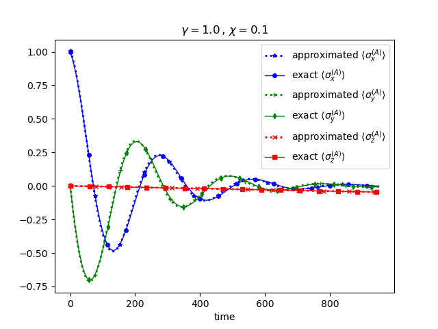
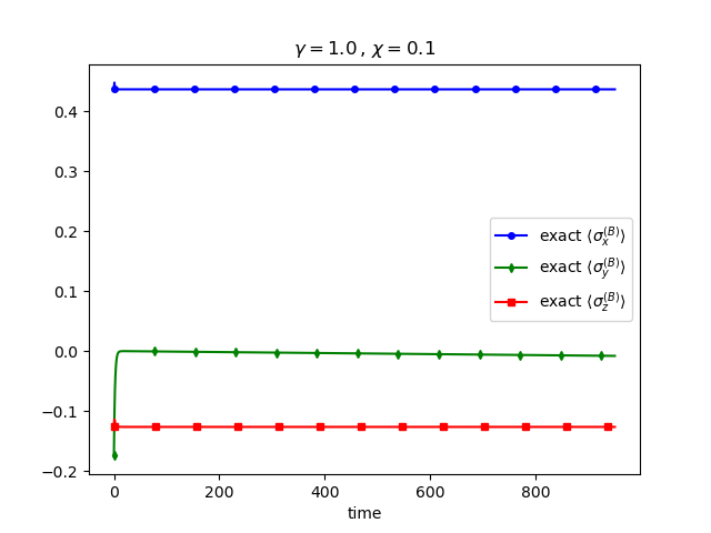
The evolution of the approximated expectation value of the Pauli matrices for qubit AA and BB for γ=1\gamma=1 and χ=0.1\chi=0.1 and with the initial state taken as

|ϕ+=12(|0+|1)\lvert\phi_{+}\rangle=\frac{1}{\sqrt{2}}\left(\lvert 0\rangle+\lvert 1\rangle\right)

are compared in Figure 1 to the ones obtained through an exact full numerical propagation. We see that the adiabatic elimination captures the exact dynamics faithfully and that indeed qubit BB reaches its steady-state before any appreciable dynamics in AA has taken place.

It is worth mentioning that when adiabatic elimination is valid, i.e. χγ\chi\ll\gamma, the exact final state of the fast qubit BB is very close to the steady state of B\mathcal{L}_{B}:

ρss(B)=limχ0ρs0(B).\rho_{ss}^{(B)}=\lim_{\chi\to 0}\rho_{s_{0}}^{(B)}. (40)

Defining the projector 𝒫B=||ρss(B)𝟙(𝟚𝔹)||\mathcal{P}_{B}=\lvert\lvert\rho_{ss}^{(B)}\rangle\rangle\langle\langle\openone^{(2B)}\rvert\rvert leads to considerable simplifications in Eq. (14) where the first term becomes zero. Thus, taking the interaction 𝒬AB𝒬\mathcal{Q}\mathcal{L}_{AB}\mathcal{Q} to be small, we only need the term n=0n=0 in Eq. (17) and taking the zero order only in (4), one can check that it leads to the same Lindblad operator derived in Azouit et al. (2017a) which is enough to obtain a very good approximation in the adiabatic limit.

Refer to caption
Refer to caption
Figure 1: Top: Evolution of the expectations values of the Pauli matrices σxA\langle\sigma_{x}^{A}\rangle (initial value = 1), σyA\langle\sigma_{y}^{A}\rangle (initial value=0) and σzA\langle\sigma_{z}^{A}\rangle (always zero) for the slow spin AA. Dashed line: Adiabatic elimination, continuous line: exact. Bottom: Evolution of the fast spin B. The initial state has been taken as |ϕ+=12(|0+|1)\lvert\phi_{+}\rangle=\frac{1}{\sqrt{2}}\left(\lvert 0\rangle+\lvert 1\rangle\right).

III.2 Open Rabi model

The open Rabi model has been considered recently by Garbe et al. Garbe et al. (2020) in a quantum metrology context. It consist in a spin-12\frac{1}{2} (with frequency Ω\Omega) interacting with one bosonic mode (frequency ω0\omega_{0}) of a cavity described by the following Hamiltonian:

HR=Ωσz+ω0aa+λ(a+a)σx,H_{R}=\Omega\sigma_{z}+\omega_{0}a^{\dagger}a+\lambda(a+a^{\dagger})\otimes\sigma_{x}, (41)

where aa (aa^{\dagger}) is the annihilation (creation) operator of the bosonic mode. The dynamics of the open Rabi model where the relaxation of the spin (at a rate Γ\Gamma^{\prime}) and the photon losses from the cavity (at a rate κ\kappa^{\prime}) are taken into account is generated by the following Lindblad operator:

(ρ)=i[HR,ρ]+Γ𝒟σ(ρ)+κ𝒟a(ρ)\mathcal{L}\left(\rho\right)=-i[H_{R},\rho]+\Gamma^{\prime}\mathcal{D}_{\sigma_{-}}\left(\rho\right)+\kappa^{\prime}\mathcal{D}_{a}\left(\rho\right) (42)

where we have used the notation

𝒟X(ρ)=XρX12XXρ12ρXX.\mathcal{D}_{X}\left(\rho\right)=X\rho X^{\dagger}-\frac{1}{2}X^{\dagger}X\rho-\frac{1}{2}\rho X^{\dagger}X.

We also assume that ΓΩ\Gamma^{\prime}\thicksim\Omega and κω0\kappa^{\prime}\thicksim\omega_{0}. If we rescale the time by dividing the above equation by Ωω0\sqrt{\Omega\omega_{0}}, and define:

g=λΩω0,η=ω0Ω,κ=κΩω0,Γ=ΓΩω0g=\dfrac{\lambda}{\sqrt{\Omega\omega_{0}}}\,,\,\eta=\sqrt{\dfrac{\omega_{0}}{\Omega}}\,,\,\kappa=\dfrac{\kappa^{\prime}}{\sqrt{\Omega\omega_{0}}}\,,\,\Gamma=\dfrac{\Gamma^{\prime}}{\sqrt{\Omega\omega_{0}}} (43)

we rewrite the Lindbladian:

(ρ)=A(ρ)+AB(ρ)+B(ρ)\mathcal{L}\left(\rho\right)=\mathcal{L}_{A}\left(\rho\right)+\mathcal{L}_{AB}\left(\rho\right)+\mathcal{L}_{B}\left(\rho\right) (44)

with :

A(ρ)=iη[aa,ρ]+κ𝒟a(ρ)B(ρ)=i1η[σz,ρ]+Γ𝒟σ(ρ)AB(ρ)=ig[(a+a)σx,ρ].\begin{split}\mathcal{L}_{A}\left(\rho\right)&=-i\eta[a^{\dagger}a,\rho]+\kappa\mathcal{D}_{a}\left(\rho\right)\\ \mathcal{L}_{B}\left(\rho\right)&=-i\dfrac{1}{\eta}[\sigma_{z},\rho]+\Gamma\mathcal{D}_{\sigma_{-}}\left(\rho\right)\\ \mathcal{L}_{AB}\left(\rho\right)&=-ig[\left(a+a^{\dagger}\right)\otimes\sigma_{x},\rho].\end{split} (45)

It has been shown that, in the limit where ω0Ω\omega_{0}\ll\Omega, this model exhibits a quantum phase transition when gg increases Hwang et al. (2015); Puebla et al. (2017); Hwang et al. (2018); Garbe et al. (2020). The critical point corresponding to g=1g=1 separates a normal phase (g<1g<1) from a superadiant phase (g>1g>1). Here we show that our method can be used to obtain an effective Lindblad operator for the boson in the normal phase after the elimination of the fast spin. After rescaling, the adiabatic limit ω0Ω\omega_{0}\ll\Omega corresponds to η0\eta\rightarrow 0.

In the normal phase (g<1g<1), the steady state of the system, which is the kernel of the Lindblad operator given by Eq. (42), is separable and unique Garbe et al. (2020). It is straight forward to verify that the steady state of B\mathcal{L}_{B} is:

||ρss(B)=|0,0\lvert\lvert\rho^{(B)}_{ss}\rangle\rangle=\lvert 0,0\rangle (46)

Following the same steps of the last example, see Appendix. B, we define the projector 𝒫B=||ρss(B)𝟙(𝟚𝔹)||\mathcal{P}_{B}=\lvert\lvert\rho^{(B)}_{ss}\rangle\rangle\langle\langle\openone^{(2B)}\rvert\rvert and we only calculate the term 𝒬B𝒬\mathcal{Q}\mathcal{L}_{B}\mathcal{Q}, the inverse of which corresponds to 𝒬𝒬1\mathcal{Q}\mathcal{L}\mathcal{Q}^{-1} up to zeroth order in Eq. (17). Simple and straightforward calculations lead to the following Lindbladian evolution of the boson:

0(ρ(A))=i[ηaa4g2ηΓ2η2+16(a+a)2,ρ(A)]+κ𝒟a(ρ(A))+4g2η2ΓΓ2η2+16𝒟(a+a)(ρ(A))\begin{split}\mathcal{L}_{0}\left(\rho^{(A)}\right)=&-i[\eta a^{\dagger}{a}-\dfrac{4g^{2}\eta}{\Gamma^{2}\eta^{2}+16}\left(a+a^{\dagger}\right)^{2},\rho^{(A)}]\\ &+\kappa\mathcal{D}_{a}\left(\rho^{(A)}\right)+\dfrac{4g^{2}\eta^{2}\Gamma}{\Gamma^{2}\eta^{2}+16}\mathcal{D}_{\left(a+a^{\dagger}\right)}\left(\rho^{(A)}\right)\end{split} (47)

which is exactly the formula derived in Garbe et al. (2020) using a completely different method, where one should take into consideration that the parameters in (42) are double those considered in Garbe et al. (2020).

IV Conclusion

We have derived a projection based adiabatic elimination method that works for bipartite systems. This work provides a direct connection to earlier work on adiabatic elimination of a subspace of the system Hilbert space Finkelstein-Shapiro et al. (2020) so that in principle now subsystems as well as sublevels can be eliminated at the same time. We have illustrated this with two simple examples of two dispersively coupled spins and the open Rabi model. In both cases, using the lowest order approximations, we have obtain the same expressions that have been previously obtained by completely different methods. We expect that this work will find applications in the case of molecules in cavities where the cavity and part of the molecular levels could be adiabatically eliminated.

Appendix A Detailed Calculation for the 2-qubit system

Here we present in detail all the calculations involved in the example presented in section III.1: first we write ||ρs(B)\lvert\lvert\rho_{s}^{(B)}\rangle\rangle in the standard basis:

||ρs(B)=\displaystyle\lvert\lvert\rho_{s}^{(B)}\rangle\rangle= 16χ2+γ2+416χ2+γ2+8|0,0+416χ2+γ2+8|1,1\displaystyle\dfrac{16\chi^{2}+\gamma^{2}+4}{16\chi^{2}+\gamma^{2}+8}\lvert 0,0\rangle+\dfrac{4}{16\chi^{2}+\gamma^{2}+8}\lvert 1,1\rangle
+\displaystyle+ 2γ+8iχ16χ2+γ2+8|0,1+2γ8iχ16χ2+γ2+8|1,0\displaystyle\dfrac{2\gamma+8i\chi}{16\chi^{2}+\gamma^{2}+8}\lvert 0,1\rangle+\dfrac{2\gamma-8i\chi}{16\chi^{2}+\gamma^{2}+8}\lvert 1,0\rangle (48)

where in this appendix we use the notation |i,j=|i|j\lvert i,j\rangle=\lvert i\rangle\otimes\lvert j\rangle to alleviate the complexity of mathematical expressions. Then, we define the necessary projectors of the partial trace, namely:

𝒫(B)=||ρs(B)𝟙(𝔹)||\mathcal{P}^{(B)}=\lvert\lvert\rho_{s}^{(B)}\rangle\rangle\langle\langle\openone^{(B)}\rvert\rvert (49)

and

𝒬(B)=\displaystyle\mathcal{Q}^{(B)}= 𝟙(𝟚𝔹)𝒫(𝔹)\displaystyle\openone^{(2B)}-\mathcal{P}^{(B)}
416χ2+γ2+8|ΨΨ+||Ψ1,1|\displaystyle\frac{4}{16\chi^{2}+\gamma^{2}+8}\left|{\Psi_{-}}\right\rangle\left\langle{\Psi_{+}}\right|-\left|{\Psi_{-}}\right\rangle\left\langle{1,1}\right|
8iχ+2γ16χ2+γ2+8|0,1Ψ+|+|0,10,1|\displaystyle-\frac{8i\chi+2\gamma}{16\chi^{2}+\gamma^{2}+8}\lvert 0,1\rangle\langle\Psi_{+}\rvert+\left|{0,1}\right\rangle\left\langle{0,1}\right|
+8iχ2γ16χ2+γ2+8|1,0Ψ+|+|1,01,0|\displaystyle+\frac{8i\chi-2\gamma}{16\chi^{2}+\gamma^{2}+8}\lvert 1,0\rangle\langle\Psi_{+}\rvert+\lvert 1,0\rangle\langle 1,0\rvert (50)

where we have defined the following vectors:

|Ψ+\displaystyle\lvert\Psi_{+}\rangle =|0,0+|1,1\displaystyle=\lvert 0,0\rangle+\lvert 1,1\rangle
|Ψ\displaystyle\lvert\Psi_{-}\rangle =|0,0|1,1\displaystyle=\lvert 0,0\rangle-\lvert 1,1\rangle (51)

Later on, it will be useful to define

|Φ+\displaystyle\lvert\Phi_{+}\rangle =|0,1+|1,0\displaystyle=\lvert 0,1\rangle+\lvert 1,0\rangle
|Φ\displaystyle\lvert\Phi_{-}\rangle =|0,1|1,0\displaystyle=\lvert 0,1\rangle-\lvert 1,0\rangle
|Θ+\displaystyle\lvert\Theta_{+}\rangle =2γ+8iχ16χ2+γ2+8|0,1+2γ8iχ16χ2+γ2+8|1,0\displaystyle=\dfrac{2\gamma+8i\chi}{16\chi^{2}+\gamma^{2}+8}\lvert 0,1\rangle+\dfrac{2\gamma-8i\chi}{16\chi^{2}+\gamma^{2}+8}\lvert 1,0\rangle
|Θ\displaystyle\lvert\Theta_{-}\rangle =2γ+8iχ16χ2+γ2+8|0,12γ8iχ16χ2+γ2+8|1,0\displaystyle=\dfrac{2\gamma+8i\chi}{16\chi^{2}+\gamma^{2}+8}\lvert 0,1\rangle-\dfrac{2\gamma-8i\chi}{16\chi^{2}+\gamma^{2}+8}\lvert 1,0\rangle
|Ω+\displaystyle\lvert\Omega_{+}\rangle =16χ2+γ2+416χ2+γ2+8|0,0+416χ2+γ2+8|1,1\displaystyle=\dfrac{16\chi^{2}+\gamma^{2}+4}{16\chi^{2}+\gamma^{2}+8}\lvert 0,0\rangle+\dfrac{4}{16\chi^{2}+\gamma^{2}+8}\lvert 1,1\rangle
|Ω\displaystyle\lvert\Omega_{-}\rangle =16χ2+γ2+416χ2+γ2+8|0,0416χ2+γ2+8|1,1\displaystyle=\dfrac{16\chi^{2}+\gamma^{2}+4}{16\chi^{2}+\gamma^{2}+8}\lvert 0,0\rangle-\dfrac{4}{16\chi^{2}+\gamma^{2}+8}\lvert 1,1\rangle
|Ω+\displaystyle\lvert\Omega^{\perp}_{+}\rangle =16χ2+γ2+416χ2+γ2+8|1,1416χ2+γ2+8|0,0\displaystyle=\dfrac{16\chi^{2}+\gamma^{2}+4}{16\chi^{2}+\gamma^{2}+8}\lvert 1,1\rangle-\dfrac{4}{16\chi^{2}+\gamma^{2}+8}\lvert 0,0\rangle
|Ω\displaystyle\lvert\Omega^{\perp}_{-}\rangle =16χ2+γ2+416χ2+γ2+8|1,1+416χ2+γ2+8|0,0\displaystyle=\dfrac{16\chi^{2}+\gamma^{2}+4}{16\chi^{2}+\gamma^{2}+8}\lvert 1,1\rangle+\dfrac{4}{16\chi^{2}+\gamma^{2}+8}\lvert 0,0\rangle (52)

and the unitary matrix:

𝒰SWAP=|0,00,0|+|1,11,1|+|1,00,1|+|0,11,0|\mathcal{U}_{\mathrm{SWAP}}=\left|{0,0}\right\rangle\left\langle{0,0}\right|+\left|{1,1}\right\rangle\left\langle{1,1}\right|+\left|{1,0}\right\rangle\left\langle{0,1}\right|+\left|{0,1}\right\rangle\left\langle{1,0}\right| (53)

as well. From Eqs. (A), (III.1) and (A), we find that:

𝒫𝒫=|0,10,1|𝒜0,1+|1,01,0|𝒜1,0𝒫𝒬=|0,10,1|𝒞0,1+|1,01,0|𝒞1,0𝒬𝒫=|0,10,1|𝒟0,1+|1,01,0|𝒟1,0+|0,00,0|𝒟0,0+|1,11,1|𝒟1,1𝒬𝒬=|0,10,1|0,1+|1,01,0|1,0+|0,00,0|0,0+|1,11,1|1,1\begin{split}\mathcal{P}\mathcal{L}\mathcal{P}=&\left|{0,1}\right\rangle\left\langle{0,1}\right|\otimes\mathcal{A}_{0,1}+\left|{1,0}\right\rangle\left\langle{1,0}\right|\otimes\mathcal{A}_{1,0}\\ \mathcal{P}\mathcal{L}\mathcal{Q}=&\left|{0,1}\right\rangle\left\langle{0,1}\right|\otimes\mathcal{C}_{0,1}+\left|{1,0}\right\rangle\left\langle{1,0}\right|\otimes\mathcal{C}_{1,0}\\ \mathcal{Q}\mathcal{L}\mathcal{P}=&\left|{0,1}\right\rangle\left\langle{0,1}\right|\otimes\mathcal{D}_{0,1}+\left|{1,0}\right\rangle\left\langle{1,0}\right|\otimes\mathcal{D}_{1,0}\\ +&\left|{0,0}\right\rangle\left\langle{0,0}\right|\otimes\mathcal{D}_{0,0}+\left|{1,1}\right\rangle\left\langle{1,1}\right|\otimes\mathcal{D}_{1,1}\\ \mathcal{Q}\mathcal{L}\mathcal{Q}=&\left|{0,1}\right\rangle\left\langle{0,1}\right|\otimes\mathcal{B}_{0,1}+\left|{1,0}\right\rangle\left\langle{1,0}\right|\otimes\mathcal{B}_{1,0}\\ +&\left|{0,0}\right\rangle\left\langle{0,0}\right|\otimes\mathcal{B}_{0,0}+\left|{1,1}\right\rangle\left\langle{1,1}\right|\otimes\mathcal{B}_{1,1}\end{split} (54)

Where we have defined the following matrices on \mathbfcal{H}^{(2B)}

𝒜0,1=\displaystyle\mathcal{A}_{0,1}= 2iχ(16χ2+γ2)(16χ2+γ2+8)𝒫(B),𝒜1,0=𝒰SWAP𝒜0,1¯\displaystyle\frac{2i\chi\left(16\chi^{2}+\gamma^{2}\right)}{\left(16\chi^{2}+\gamma^{2}+8\right)}\mathcal{P}^{(B)}\,,\,\mathcal{A}_{1,0}=\mathcal{U}_{\mathrm{SWAP}}\overline{\mathcal{A}_{0,1}} (55)
𝒞0,1=\displaystyle\mathcal{C}_{0,1}= 4iχ|ρs(B)Ω+|,𝒞1,0=𝒰SWAP𝒞0,1¯\displaystyle-4i\chi\lvert\rho_{s}^{(B)}\rangle\langle\Omega^{\perp}_{+}\rvert\,,\,\mathcal{C}_{1,0}=\mathcal{U}_{\mathrm{SWAP}}\overline{\mathcal{C}_{0,1}} (56)
𝒟0,1=\displaystyle\mathcal{D}_{0,1}= 16iχ(16χ2+γ2+4)(16χ2+γ2+8)2|ΨΨ+|4iχ(16χ2+γ2)(16χ2+γ2+8)|Θ+Ψ+|2iχ|ΘΨ+|\displaystyle\frac{16i\chi\left(16\chi^{2}+\gamma^{2}+4\right)}{\left(16\chi^{2}+\gamma^{2}+8\right)^{2}}\left|{\Psi_{-}}\right\rangle\left\langle{\Psi_{+}}\right|-\frac{4i\chi\left(16\chi^{2}+\gamma^{2}\right)}{\left(16\chi^{2}+\gamma^{2}+8\right)}\left|{\Theta_{+}}\right\rangle\left\langle{\Psi_{+}}\right|-2i\chi\left|{\Theta_{-}}\right\rangle\left\langle{\Psi_{+}}\right|
𝒟1,1=\displaystyle\mathcal{D}_{1,1}= 4iχ|ΘΨ+|,𝒟1,0=𝒰SWAP𝒟0,1¯,𝒟0,0=𝟎\displaystyle-4i\chi\left|{\Theta_{-}}\right\rangle\left\langle{\Psi_{+}}\right|\,,\,\mathcal{D}_{1,0}=\mathcal{U}_{\mathrm{SWAP}}\overline{\mathcal{D}_{0,1}}\,,\,\mathcal{D}_{0,0}=\mathbf{0} (57)
0,1=\displaystyle\mathcal{B}_{0,1}= 2iχ(16χ2+γ2)(16χ2+γ2+8)|ΨΩ+|+γ|Ψ1,1|γ2|0,10,1|γ2|1,01,0||ΨΦ+|+|Φ+Ψ|\displaystyle\frac{2i\chi\left(16\chi^{2}+\gamma^{2}\right)}{\left(16\chi^{2}+\gamma^{2}+8\right)}\left|{\Psi_{-}}\right\rangle\left\langle{\Omega^{\perp}_{+}}\right|+\gamma\left|{\Psi_{-}}\right\rangle\left\langle{1,1}\right|-\frac{\gamma}{2}\left|{0,1}\right\rangle\left\langle{0,1}\right|-\frac{\gamma}{2}\left|{1,0}\right\rangle\left\langle{1,0}\right|-\left|{\Psi_{-}}\right\rangle\left\langle{\Phi_{+}}\right|+\left|{\Phi_{+}}\right\rangle\left\langle{\Psi_{-}}\right|
+2iχ(16χ2+γ2)(16χ2+γ2+8)|ΘΨ|+64iχ(4iχγ)(16χ2+γ2+8)2|1,00,0|+16iχ(4iχ+γ)(16χ2+γ2+4)(16χ2+γ2+8)2|0,11,1|\displaystyle+\frac{2i\chi\left(16\chi^{2}+\gamma^{2}\right)}{\left(16\chi^{2}+\gamma^{2}+8\right)}\left|{\Theta_{-}}\right\rangle\left\langle{\Psi_{-}}\right|+\frac{64i\chi\left(4i\chi-\gamma\right)}{\left(16\chi^{2}+\gamma^{2}+8\right)^{2}}\left|{1,0}\right\rangle\left\langle{0,0}\right|+\frac{16i\chi\left(4i\chi+\gamma\right)\left(16\chi^{2}+\gamma^{2}+4\right)}{\left(16\chi^{2}+\gamma^{2}+8\right)^{2}}\left|{0,1}\right\rangle\left\langle{1,1}\right|
0,0=\displaystyle\mathcal{B}_{0,0}= |ΨΦ+|+|Φ+Ψ|+γ|Ψ1,1|+4iχγ2|0,10,1|4iχ+γ2|1,01,0|\displaystyle-\left|{\Psi_{-}}\right\rangle\left\langle{\Phi_{+}}\right|+\left|{\Phi_{+}}\right\rangle\left\langle{\Psi_{-}}\right|+\gamma\left|{\Psi_{-}}\right\rangle\left\langle{1,1}\right|+\frac{4i\chi-\gamma}{2}\left|{0,1}\right\rangle\left\langle{0,1}\right|-\frac{4i\chi+\gamma}{2}\left|{1,0}\right\rangle\left\langle{1,0}\right|
1,1=\displaystyle\mathcal{B}_{1,1}= 0,0+4iχ(|ΘΨ+|+|1,01,0||0,10,1|),1,0=𝒰SWAP0,1¯𝒰SWAP\displaystyle\mathcal{B}_{0,0}+4i\chi\left(\left|{\Theta_{-}}\right\rangle\left\langle{\Psi_{+}}\right|+\left|{1,0}\right\rangle\left\langle{1,0}\right|-\left|{0,1}\right\rangle\left\langle{0,1}\right|\right)\,,\,\mathcal{B}_{1,0}=\mathcal{U}_{\mathrm{SWAP}}\overline{\mathcal{B}_{0,1}}\mathcal{U}_{\mathrm{SWAP}} (58)

With this diagonal form of 𝒬𝒬\mathcal{Q}\mathcal{L}\mathcal{Q}, it is straightforward to compute (𝒬𝒬)1\left(\mathcal{Q}\mathcal{L}\mathcal{Q}\right)^{-1}. It consists in computing i,j1\mathcal{B}_{i,j}^{-1}, i,j=0,1i,j=0,1, which are 4×44\times 4 matrices. Moreover, since we are solely interested in quantities of the form 𝒫𝒬(𝒬𝒬)n𝒬𝒫\mathcal{P}\mathcal{L}\mathcal{Q}\left(\mathcal{Q}\mathcal{L}\mathcal{Q}\right)^{-n}\mathcal{Q}\mathcal{L}\mathcal{P} and 𝒫𝒬\mathcal{P}\mathcal{L}\mathcal{Q} is of the form (26), we only need to compute 0,1\mathcal{B}_{0,1}.
To simplify this task, we define the unitary matrix

𝒰=12|0,0Ψ+|12|1,1Ψ|+|0,10,1|+|1,01,0|,\mathcal{U}=\frac{1}{\sqrt{2}}\left|{0,0}\right\rangle\left\langle{\Psi_{+}}\right|-\frac{1}{\sqrt{2}}\left|{1,1}\right\rangle\left\langle{\Psi_{-}}\right|+\left|{0,1}\right\rangle\left\langle{0,1}\right|+\left|{1,0}\right\rangle\left\langle{1,0}\right|, (59)

and we compute the pseudo-inverse of ~0,1=𝒰0,1\tilde{\mathcal{B}}_{0,1}=\mathcal{U}\mathcal{B}_{0,1}. Multiplying by 𝒰\mathcal{U} boils down to replacing the ket |Ψ\lvert\Psi_{-}\rangle by |1,1\lvert 1,1\rangle in (A), which implies that ~0,1\tilde{\mathcal{B}}_{0,1} can be represented as a 3×43\times 4 matrix in the standard basis ”simplifying” the task of finding ~0,11\tilde{\mathcal{B}}_{0,1}^{-1}. To find the pseudo inverse of ~0,1\tilde{\mathcal{B}}_{0,1}, we simply solve the set of equations corresponding to:

~0,1~0,11=Πran[~0,1]=𝟙(𝟚𝔹)|𝟘,𝟘𝟘,𝟘|\tilde{\mathcal{B}}_{0,1}\tilde{\mathcal{B}}_{0,1}^{-1}=\Pi_{\text{ran}[\tilde{\mathcal{B}}_{0,1}]}=\openone^{(2B)}-\left|{0,0}\right\rangle\left\langle{0,0}\right| (60)

where Πran[~0,1]\Pi_{\text{ran}[\tilde{\mathcal{B}}_{0,1}]} is the hermitian projector to the range of ~0,1\tilde{\mathcal{B}}_{0,1}. If we define the following quantities

b11\displaystyle b_{11} =γ(16χ2+γ2+8)22(2iχγ(16χ2+γ216)+(γ2+8)(16χ2+γ2+8))(16χ2+γ2+4)\displaystyle=-\frac{\gamma\left(16\chi^{2}+\gamma^{2}+8\right)^{2}}{\sqrt{2}\left(2i\chi\gamma\left(16\chi^{2}+\gamma^{2}-16\right)+\left(\gamma^{2}+8\right)\left(16\chi^{2}+\gamma^{2}+8\right)\right)\left(16\chi^{2}+\gamma^{2}+4\right)} (61)
b21\displaystyle b_{21} =2(16χ2γ2+256χ24iχγ(16χ2+γ2)+γ4+16γ2+64)(2iχγ(16χ2+γ216)+(γ2+8)(16χ2+γ2+8))(16χ2+γ2+4)\displaystyle=\frac{\sqrt{2}\left(16\chi^{2}\gamma^{2}+256\chi^{2}-4i\chi\gamma\left(16\chi^{2}+\gamma^{2}\right)+\gamma^{4}+16\gamma^{2}+64\right)}{\left(2i\chi\gamma\left(16\chi^{2}+\gamma^{2}-16\right)+\left(\gamma^{2}+8\right)\left(16\chi^{2}+\gamma^{2}+8\right)\right)\left(16\chi^{2}+\gamma^{2}+4\right)} (62)
b31\displaystyle b_{31} =2(16χ2γ24iχγ(48χ2+3γ2+16)+(32χ2+γ2+8)2)(2iχγ(16χ2+γ216)+(γ2+8)(16χ2+γ2+8))(16χ2+γ2+4)\displaystyle=\frac{\sqrt{2}\left(16\chi^{2}\gamma^{2}-4i\chi\gamma\left(48\chi^{2}+3\gamma^{2}+16\right)+\left(32\chi^{2}+\gamma^{2}+8\right)^{2}\right)}{\left(2i\chi\gamma\left(16\chi^{2}+\gamma^{2}-16\right)+\left(\gamma^{2}+8\right)\left(16\chi^{2}+\gamma^{2}+8\right)\right)\left(16\chi^{2}+\gamma^{2}+4\right)} (63)
b33\displaystyle b_{33} =512χ4γ2+64χ2γ4+576χ2γ2+1024χ2+4iχγ(16χ2+γ2)2+2γ6+36γ4+192γ2+256γ(2iχγ(16χ2+γ216)+(γ2+8)(16χ2+γ2+8))(16χ2+γ2+4)\displaystyle=-\frac{512\chi^{4}\gamma^{2}+64\chi^{2}\gamma^{4}+576\chi^{2}\gamma^{2}+1024\chi^{2}+4i\chi\gamma\left(16\chi^{2}+\gamma^{2}\right)^{2}+2\gamma^{6}+36\gamma^{4}+192\gamma^{2}+256}{\gamma\left(2i\chi\gamma\left(16\chi^{2}+\gamma^{2}-16\right)+\left(\gamma^{2}+8\right)\left(16\chi^{2}+\gamma^{2}+8\right)\right)\left(16\chi^{2}+\gamma^{2}+4\right)} (64)
b22\displaystyle b_{22} =b3332χ(8χ(16χ2+γ2+4)iγ(16χ2+γ2+8))γ(2iχγ(16χ2+γ216)+(γ2+8)(16χ2+γ2+8))(16χ2+γ2+4)\displaystyle=b_{33}-\frac{32\chi\left(8\chi\left(16\chi^{2}+\gamma^{2}+4\right)-i\gamma\left(16\chi^{2}+\gamma^{2}+8\right)\right)}{\gamma\left(2i\chi\gamma\left(16\chi^{2}+\gamma^{2}-16\right)+\left(\gamma^{2}+8\right)\left(16\chi^{2}+\gamma^{2}+8\right)\right)\left(16\chi^{2}+\gamma^{2}+4\right)} (65)
b12\displaystyle b_{12} =b13=22γb11,b23=22γb21,b32=22γb31\displaystyle=b_{13}=\frac{2\sqrt{2}}{\gamma}b_{11}\,,\,b_{23}=\frac{2\sqrt{2}}{\gamma}b_{21}\,,\,b_{32}=\frac{2\sqrt{2}}{\gamma}b_{31} (66)

and make the identification |1,1|1\lvert 1,1\rangle\rightarrow\lvert 1\rangle, |1,0|2\lvert 1,0\rangle\rightarrow\lvert 2\rangle and |0,1|3\lvert 0,1\rangle\rightarrow\lvert 3\rangle, then:

~0,11=i,j=13bij|ij|\tilde{\mathcal{B}}_{0,1}^{-1}=\sum_{i,j=1}^{3}b_{ij}\left|{i}\right\rangle\left\langle{j}\right| (67)

We can check that ~0,11\tilde{\mathcal{B}}_{0,1}^{-1} verify all the Moore-Penrose conditions Penrose (1955):

~0,1~0,11~0,1=~0,1,~0,11~0,1~0,11=~0,11(~0,1~0,11)=~0,1~0,11,(~0,11~0,1)=~0,11~0,1\begin{split}\tilde{\mathcal{B}}_{0,1}\tilde{\mathcal{B}}_{0,1}^{-1}\tilde{\mathcal{B}}_{0,1}=\tilde{\mathcal{B}}_{0,1}&,\tilde{\mathcal{B}}_{0,1}^{-1}\tilde{\mathcal{B}}_{0,1}\tilde{\mathcal{B}}_{0,1}^{-1}=\tilde{\mathcal{B}}_{0,1}^{-1}\\ \left(\tilde{\mathcal{B}}_{0,1}\tilde{\mathcal{B}}_{0,1}^{-1}\right)^{\dagger}=\tilde{\mathcal{B}}_{0,1}\tilde{\mathcal{B}}_{0,1}^{-1},&\left(\tilde{\mathcal{B}}_{0,1}^{-1}\tilde{\mathcal{B}}_{0,1}\right)^{\dagger}=\tilde{\mathcal{B}}_{0,1}^{-1}\tilde{\mathcal{B}}_{0,1}\end{split} (68)

Finally, we can easily see that the pseudo-inverse of 0,1{\mathcal{B}}_{0,1} is:

0,11=(𝒰~0,1)1=~0,11𝒰{\mathcal{B}}_{0,1}^{-1}=\left(\mathcal{U}^{\dagger}\tilde{\mathcal{B}}_{0,1}\right)^{-1}=\tilde{\mathcal{B}}_{0,1}^{-1}\mathcal{U} (69)

with that, we have all the necessary ingredients to compute 0\mathcal{L}_{0} and 1\mathcal{L}_{1}. Using Eqs.(54), we find that:

0=𝒫𝒫𝒫𝒬(𝒬𝒬)1𝒬𝒫=|0,10,1|[𝒜0,1𝒞0,10,11𝒟0,1]+|1,01,0|[𝒜1,0𝒞1,01,01𝒟1,0]\begin{split}\mathcal{L}_{0}&=\mathcal{P}\mathcal{L}\mathcal{P}-\mathcal{P}\mathcal{L}\mathcal{Q}\left(\mathcal{Q}\mathcal{L}\mathcal{Q}\right)^{-1}\mathcal{Q}\mathcal{L}\mathcal{P}\\ &=\left|{0,1}\right\rangle\left\langle{0,1}\right|\otimes\left[\mathcal{A}_{0,1}-\mathcal{C}_{0,1}\mathcal{B}^{-1}_{0,1}\mathcal{D}_{0,1}\right]\\ &+\left|{1,0}\right\rangle\left\langle{1,0}\right|\otimes\left[\mathcal{A}_{1,0}-\mathcal{C}_{1,0}\mathcal{B}^{-1}_{1,0}\mathcal{D}_{1,0}\right]\end{split} (70)
1=𝒫𝒬(𝒬𝒬)2𝒬𝒫=|0,10,1|[𝒞0,10,12𝒟0,1]|1,01,0|[𝒞1,01,02𝒟1,0]\begin{split}\mathcal{L}_{1}&=-\mathcal{P}\mathcal{L}\mathcal{Q}\left(\mathcal{Q}\mathcal{L}\mathcal{Q}\right)^{-2}\mathcal{Q}\mathcal{L}\mathcal{P}\\ &=-\left|{0,1}\right\rangle\left\langle{0,1}\right|\otimes\left[\mathcal{C}_{0,1}\mathcal{B}^{-2}_{0,1}\mathcal{D}_{0,1}\right]\\ &-\left|{1,0}\right\rangle\left\langle{1,0}\right|\otimes\left[\mathcal{C}_{1,0}\mathcal{B}^{-2}_{1,0}\mathcal{D}_{1,0}\right]\end{split} (71)

Since 𝒫(B)\mathcal{P}^{(B)} is a projector of rank 11, we can write:

𝒜0,1𝒞0,10,11𝒟0,1=α0,1𝒫(B)𝒜1,0𝒞1,01,01𝒟1,0=α1,0𝒫(B)𝒞0,10,12𝒟0,1=β0,1𝒫(B)𝒞1,01,02𝒟1,0=β1,0𝒫(B)\begin{split}\mathcal{A}_{0,1}-\mathcal{C}_{0,1}\mathcal{B}^{-1}_{0,1}\mathcal{D}_{0,1}&=\alpha_{0,1}\mathcal{P}^{(B)}\\ \mathcal{A}_{1,0}-\mathcal{C}_{1,0}\mathcal{B}^{-1}_{1,0}\mathcal{D}_{1,0}&=\alpha_{1,0}\mathcal{P}^{(B)}\\ \mathcal{C}_{0,1}\mathcal{B}^{-2}_{0,1}\mathcal{D}_{0,1}&=\beta_{0,1}\mathcal{P}^{(B)}\\ \mathcal{C}_{1,0}\mathcal{B}^{-2}_{1,0}\mathcal{D}_{1,0}&=\beta_{1,0}\mathcal{P}^{(B)}\end{split} (72)

Because 𝒫B\mathcal{P}_{B} is of the form |ρs0(B)Ψ+|\lvert\rho^{(B)}_{s_{0}}\rangle\langle\Psi_{+}\rvert, we find that:

α0,1α=12Ψ+|(𝒜0,1𝒞0,10,11𝒟0,1)|Ψ+β0,1β=12Ψ+|(𝒞0,10,12𝒟0,1)|Ψ+\begin{split}\alpha_{0,1}&\equiv\alpha=\frac{1}{2}\langle\Psi_{+}\rvert\left(\mathcal{A}_{0,1}-\mathcal{C}_{0,1}\mathcal{B}^{-1}_{0,1}\mathcal{D}_{0,1}\right)\lvert\Psi_{+}\rangle\\ \beta_{0,1}&\equiv\beta=\frac{1}{2}\langle\Psi_{+}\rvert\left(\mathcal{C}_{0,1}\mathcal{B}^{-2}_{0,1}\mathcal{D}_{0,1}\right)\lvert\Psi_{+}\rangle\end{split} (73)

where we have used the fact that Ψ+|ρs0(B)=1\langle\Psi_{+}\rvert\rho^{(B)}_{s_{0}}\rangle=1 and Ψ+|Ψ+=2\langle\Psi_{+}\rvert\Psi_{+}\rangle=2. We also have:

α1,0=12Ψ+|(𝒜1,0𝒞1,01,01𝒟1,0)|Ψ+=12Ψ+|(𝒰SWAP𝒜0,1¯𝒰SWAP𝒞0,1¯𝒰SWAP0,11¯𝒟0,1¯)|Ψ+=12Ψ+|(𝒜0,1¯𝒞0,1¯0,11¯𝒟0,1¯)|Ψ+=α¯\begin{split}\alpha_{1,0}&=\frac{1}{2}\langle\Psi_{+}\rvert\left(\mathcal{A}_{1,0}-\mathcal{C}_{1,0}\mathcal{B}^{-1}_{1,0}\mathcal{D}_{1,0}\right)\lvert\Psi_{+}\rangle\\ &=\frac{1}{2}\langle\Psi_{+}\rvert\left(\mathcal{U}_{\mathrm{SWAP}}\overline{\mathcal{A}_{0,1}}-\mathcal{U}_{\mathrm{SWAP}}\overline{\mathcal{C}_{0,1}}\mathcal{U}_{\mathrm{SWAP}}\overline{\mathcal{B}_{0,1}^{-1}}\overline{\mathcal{D}_{0,1}}\right)\lvert\Psi_{+}\rangle\\ &=\frac{1}{2}\langle\Psi_{+}\rvert\left(\overline{\mathcal{A}_{0,1}}-\overline{\mathcal{C}_{0,1}}\overline{\mathcal{B}_{0,1}^{-1}}\overline{\mathcal{D}_{0,1}}\right)\lvert\Psi_{+}\rangle=\overline{\alpha}\end{split} (74)

where we have used the fact that 𝒰SWAP2=𝟙(𝟚𝔹)\mathcal{U}_{\mathrm{SWAP}}^{2}=\openone^{(2B)}, 𝒞0,1¯𝒰SWAP=𝒞0,1¯\overline{\mathcal{C}_{0,1}}\mathcal{U}_{\mathrm{SWAP}}=\overline{\mathcal{C}_{0,1}}, and Ψ+|𝒰SWAP=Ψ+|\langle\Psi_{+}\rvert\mathcal{U}_{\mathrm{SWAP}}=\langle\Psi_{+}\rvert. In a similar way we can also show that:

β1,0=β¯\beta_{1,0}=\overline{\beta} (75)

Let us define α=ζ+iξ\alpha=-\zeta+i\xi where ζ0\zeta\geq 0. A tedious calculation leads to:

ζ=128χ2γ(γ2+8)(16χ2+γ2+2)4χ2γ2(16χ2+γ216)2+(γ2+8)2(16χ2+γ2+8)2ξ=2χ(16χ2+γ2)16χ2+γ2+8+256χ3γ2(16χ2+γ216)(16χ2+γ2+2)(4χ2γ2(16χ2+γ216)2+(γ2+8)2(16χ2+γ2+8)2)(16χ2+γ2+8)\begin{split}\zeta&=\frac{128\chi^{2}\gamma\left(\gamma^{2}+8\right)\left(16\chi^{2}+\gamma^{2}+2\right)}{4\chi^{2}\gamma^{2}\left(16\chi^{2}+\gamma^{2}-16\right)^{2}+\left(\gamma^{2}+8\right)^{2}\left(16\chi^{2}+\gamma^{2}+8\right)^{2}}\\ \xi&=\frac{2\chi\left(16\chi^{2}+\gamma^{2}\right)}{16\chi^{2}+\gamma^{2}+8}+\frac{256\chi^{3}\gamma^{2}\left(16\chi^{2}+\gamma^{2}-16\right)\left(16\chi^{2}+\gamma^{2}+2\right)}{\left(4\chi^{2}\gamma^{2}\left(16\chi^{2}+\gamma^{2}-16\right)^{2}+\left(\gamma^{2}+8\right)^{2}\left(16\chi^{2}+\gamma^{2}+8\right)^{2}\right)\left(16\chi^{2}+\gamma^{2}+8\right)}\end{split} (76)

and

β=x1+iy1x2+iy2\beta=\frac{x_{1}+iy_{1}}{x_{2}+iy_{2}}

where

x1=χ2(49152χ4γ2262144χ4+6144χ2γ4+2048χ2γ2131072χ2+192γ6+1152γ45120γ216384)y1=256χ3γ(16χ2+γ2+4)(16χ2+γ2+8)x2=(16χ2+γ2+4)(32χ3γ+16χ2γ2+128χ22χγ3+32χγ+γ4+16γ2+64)×(32χ3γ+16χ2γ2+128χ2+2χγ332χγ+γ4+16γ2+64)y2=4χγ(γ2+8)(16χ2+γ216)(16χ2+γ2+4)(16χ2+γ2+8)\begin{split}x_{1}=&\chi^{2}\left(49152\chi^{4}\gamma^{2}-262144\chi^{4}+6144\chi^{2}\gamma^{4}+2048\chi^{2}\gamma^{2}-131072\chi^{2}+192\gamma^{6}+1152\gamma^{4}-5120\gamma^{2}-16384\right)\\ y_{1}=&256\chi^{3}\gamma\left(16\chi^{2}+\gamma^{2}+4\right)\left(16\chi^{2}+\gamma^{2}+8\right)\\ x_{2}=&\left(16\chi^{2}+\gamma^{2}+4\right)\left(-32\chi^{3}\gamma+16\chi^{2}\gamma^{2}+128\chi^{2}-2\chi\gamma^{3}+32\chi\gamma+\gamma^{4}+16\gamma^{2}+64\right)\\ &\times\left(32\chi^{3}\gamma+16\chi^{2}\gamma^{2}+128\chi^{2}+2\chi\gamma^{3}-32\chi\gamma+\gamma^{4}+16\gamma^{2}+64\right)\\ y_{2}=&4\chi\gamma\left(\gamma^{2}+8\right)\left(16\chi^{2}+\gamma^{2}-16\right)\left(16\chi^{2}+\gamma^{2}+4\right)\left(16\chi^{2}+\gamma^{2}+8\right)\end{split} (77)

Finally, it is straightforward to calculate (𝟙𝟙)1\left(\openone-\mathcal{L}_{1}\right)^{-1} exactly , given that 1\mathcal{L}_{1} (71) is block diagonal:

(𝟙𝟙)1=|0,10,1|[11+β𝒫B+𝒬B]+|1,01,0|[11+β¯𝒫B+𝒬B]+[|0,00,0|+|1,11,1|]𝟙(𝟚𝔹)\begin{split}\left(\openone-\mathcal{L}_{1}\right)^{-1}&=\left|{0,1}\right\rangle\left\langle{0,1}\right|\otimes\left[\frac{1}{1+\beta}\mathcal{P}_{B}+\mathcal{Q}_{B}\right]\\ &+\left|{1,0}\right\rangle\left\langle{1,0}\right|\otimes\left[\frac{1}{1+\overline{\beta}}\mathcal{P}_{B}+\mathcal{Q}_{B}\right]\\ &+\left[\left|{0,0}\right\rangle\left\langle{0,0}\right|+\left|{1,1}\right\rangle\left\langle{1,1}\right|\right]\otimes\openone^{(2B)}\end{split} (78)

Taking the fact 𝒬Bρs0(B)=0\mathcal{Q}_{B}\rho^{(B)}_{s_{0}}=0 into account and defining the modified initial state of the qubit AA as:

|ρ~0(A)=ρ0,0|0,0+ρ1,1|1,1+ρ0,11+β|0,1+ρ1,01+β¯|1,0,\lvert\tilde{\rho}^{(A)}_{0}\rangle=\rho_{0,0}\lvert 0,0\rangle+\rho_{1,1}\lvert 1,1\rangle+\frac{\rho_{0,1}}{1+\beta}\lvert 0,1\rangle+\frac{\rho_{1,0}}{1+\overline{\beta}}\lvert 1,0\rangle, (79)

where ρ0,0,ρ1,1\rho_{0,0},\rho_{1,1} represent population in the state ρ0(A)\rho^{(A)}_{0} while ρ0,1,ρ1,0\rho_{0,1},\rho_{1,0} represent initial coherences, we can simplify (6) to describe the dynamics of the slow qubit as:

|ρA(t)=eL~0t|ρ~0A,\lvert\rho^{A}(t)\rangle=e^{\tilde{L}_{0}t}\lvert\tilde{\rho}^{A}_{0}\rangle, (80)

where L~0=α1+β|0,10,1|+α¯1+β¯|1,01,0|\tilde{L}_{0}=\frac{\alpha}{1+\beta}\left|{0,1}\right\rangle\left\langle{0,1}\right|+\frac{\overline{\alpha}}{1+\overline{\beta}}\left|{1,0}\right\rangle\left\langle{1,0}\right|. The evolution operator U(t)=eL~0tU(t)=e^{\tilde{L}_{0}t} is simple to calculate:

U(t)=eζt+iξt|0,10,1|+eζtiξt|1,01,0|+|0,00,0|+|1,11,1|\begin{split}U(t)&=e^{-\zeta^{\prime}t+i\xi^{\prime}t}\left|{0,1}\right\rangle\left\langle{0,1}\right|+e^{-\zeta^{\prime}t-i\xi^{\prime}t}\left|{1,0}\right\rangle\left\langle{1,0}\right|\\ &+\left|{0,0}\right\rangle\left\langle{0,0}\right|+\left|{1,1}\right\rangle\left\langle{1,1}\right|\end{split} (81)

where we have defined

ζ=α1+β,ξ=α1+β\zeta^{\prime}=-\Re{\frac{\alpha}{1+\beta}}\,,\,\xi^{\prime}=\Im{\frac{\alpha}{1+\beta}} (82)

Appendix B open Rabi model

In this section, we carry out all the calculations needed to adiabatically eliminate a fast qubit interacting with a slow cavity mode according to the open Rabi model:

(ρ)=i1η[σz,ρ]+Γ𝒟σ(ρ)iη[aa,](ρ)+κ𝒟a(ρ)ig[(a+a)σx,ρ]\begin{split}\mathcal{L}\left(\rho\right)=&-i\frac{1}{\eta}[\sigma_{z},\rho]+\Gamma\mathcal{D}_{\sigma_{-}}\left(\rho\right)-i{\eta}[a^{\dagger}a,\left](\rho\right)\\ &+\kappa\mathcal{D}_{a}\left(\rho\right)-ig[\left(a+a^{\dagger}\right)\otimes\sigma_{x},\rho]\end{split} (83)

The first step is to write \mathcal{L} in the super-operator representation:

=iη(𝟙(𝔸)𝕒𝕒𝟙(𝟚𝔹)𝕒𝕒𝟙(𝔸)𝟙(𝟚𝔹))iη(𝟙(𝟚𝔸)𝟙(𝔹)σ𝕫𝟙(𝟚𝔸)σ𝕫𝟙(𝔹))ig(𝟙(𝔸)(𝕒+𝕒)𝟙(𝔹)σ𝕩(𝕒+𝕒)𝟙(𝔸)σ𝕩𝟙(𝔹))+Γ𝟙(𝟚𝔸)σσΓ𝟚[𝟙(𝟚𝔸)σ+σ𝟙(𝔹)+𝟙(𝟚𝔸)𝟙(𝔹)σ+σ]+κaa𝟙(𝟚𝔹)κ𝟚[𝕒𝕒𝟙(𝔸)𝟙(𝟚𝔹)+𝟙(𝔸)𝕒𝕒𝟙(𝟚𝔹)]\begin{split}\mathcal{L}=&-i\eta\left(\openone^{(A)}\otimes a^{\dagger}a\otimes\openone^{(2B)}-a^{\dagger}a\otimes\openone^{(A)}\otimes\openone^{(2B)}\right)-\dfrac{i}{\eta}\left(\openone^{(2A)}\otimes\openone^{(B)}\otimes\sigma_{z}-\openone^{(2A)}\otimes\sigma_{z}\otimes\openone^{(B)}\right)\\ &-ig\left(\openone^{(A)}\otimes\left(a+a^{\dagger}\right)\otimes\openone^{(B)}\otimes\sigma_{x}-\left(a+a^{\dagger}\right)\otimes\openone^{(A)}\otimes\sigma_{x}\otimes\openone^{(B)}\right)\\ &+\Gamma\openone^{(2A)}\otimes\sigma_{-}\otimes\sigma_{-}-\dfrac{\Gamma}{2}\left[\openone^{(2A)}\otimes\sigma_{+}\sigma_{-}\otimes\openone^{(B)}+\openone^{(2A)}\otimes\openone^{(B)}\otimes\sigma_{+}\sigma_{-}\right]\\ &+\kappa a\otimes a\otimes\openone^{(2B)}-\dfrac{\kappa}{2}\left[a^{\dagger}a\otimes\openone^{(A)}\otimes\openone^{(2B)}+\openone^{(A)}\otimes a^{\dagger}a\otimes\openone^{(2B)}\right]\end{split}

If we define:

𝒫B=||ρfB𝟙(𝔹)||,𝒬𝔹=𝟙(𝟚𝔹)𝒫𝔹=|𝟙,𝟙𝟙,𝟙||𝟘,𝟘𝟙,𝟙|+|𝟘,𝟙𝟘,𝟙|+|𝟙,𝟘𝟙,𝟘|\mathcal{P}_{B}=\lvert\lvert\rho^{B}_{f}\rangle\rangle\langle\langle\openone^{(B)}\rvert\rvert\,,\,\mathcal{Q}_{B}=\openone^{(2B)}-\mathcal{P}_{B}=\left|{1,1}\right\rangle\left\langle{1,1}\right|-\left|{0,0}\right\rangle\left\langle{1,1}\right|+\left|{0,1}\right\rangle\left\langle{0,1}\right|+\left|{1,0}\right\rangle\left\langle{1,0}\right| (84)

and

𝒫=𝟙(𝟚𝔸)𝒫𝔹,𝒬=𝟙(𝟚𝔸)𝒬𝔹\mathcal{P}=\openone^{(2A)}\otimes\mathcal{P}_{B}\,,\,\mathcal{Q}=\openone^{(2A)}\otimes\mathcal{Q}_{B} (85)

then we can compute the needed quantities for 0\mathcal{L}_{0}

𝒫𝒫=\displaystyle\mathcal{P}\mathcal{L}\mathcal{P}= [iη(𝟙(𝔸)𝕒𝕒𝕒𝕒𝟙(𝔸))+κaaκ2[aa𝟙(𝔸)+𝟙(𝔸)𝕒𝕒]]PB\displaystyle\left[-i\eta\left(\openone^{(A)}\otimes a^{\dagger}a-a^{\dagger}a\otimes\openone^{(A)}\right)+\kappa a\otimes a-\dfrac{\kappa}{2}\left[a^{\dagger}a\otimes\openone^{(A)}+\openone^{(A)}\otimes a^{\dagger}a\right]\right]\otimes P_{B}
𝒫𝒬=\displaystyle\mathcal{P}\mathcal{L}\mathcal{Q}= ig[𝟙(𝔸)(𝕒+𝕒)(𝕒+𝕒)𝟙(𝔸)]|0,0Φ+|\displaystyle-ig\left[\openone^{(A)}\otimes\left(a+a^{\dagger}\right)-\left(a+a^{\dagger}\right)\otimes\openone^{(A)}\right]\otimes\left|{0,0}\right\rangle\left\langle{\Phi_{+}}\right|
𝒬𝒫=\displaystyle\mathcal{Q}\mathcal{L}\mathcal{P}= ig(𝟙(𝔸)(𝕒+𝕒)|𝟘,𝟙Ψ+|(𝕒+𝕒)𝟙(𝔸)|𝟙,𝟘Ψ+|)\displaystyle-ig\left(\openone^{(A)}\otimes\left(a+a^{\dagger}\right)\otimes\left|{0,1}\right\rangle\left\langle{\Psi_{+}}\right|-\left(a+a^{\dagger}\right)\otimes\openone^{(A)}\otimes\left|{1,0}\right\rangle\left\langle{\Psi_{+}}\right|\right)
𝒬B𝒬\displaystyle\mathcal{Q}\mathcal{L}_{B}\mathcal{Q} =𝟙(𝟚𝔸)[Γ|𝟙,𝟙𝟙,𝟙|+Γ|𝟘,𝟘𝟙,𝟙|(Γ𝟚+𝟚𝕚η)|𝟘,𝟙𝟘,𝟙|(Γ𝟚𝟚𝕚η)|𝟙,𝟘𝟙,𝟘|]\displaystyle=\openone^{(2A)}\otimes\left[-\Gamma\left|{1,1}\right\rangle\left\langle{1,1}\right|+\Gamma\left|{0,0}\right\rangle\left\langle{1,1}\right|-\left(\dfrac{\Gamma}{2}+\dfrac{2i}{\eta}\right)\left|{0,1}\right\rangle\left\langle{0,1}\right|-\left(\dfrac{\Gamma}{2}-\dfrac{2i}{\eta}\right)\left|{1,0}\right\rangle\left\langle{1,0}\right|\right] (86)

𝒬B𝒬\mathcal{Q}\mathcal{L}_{B}\mathcal{Q} represents the dominant term of 𝒬𝒬\mathcal{Q}\mathcal{L}\mathcal{Q} which can be inverted quite easily:

QBQ1=𝟙(𝟚𝔸)[𝟙𝟚Γ|𝟙,𝟙𝟙,𝟙|+𝟙𝟚Γ|𝟙,𝟙𝟘,𝟘|𝟙(Γ𝟚+𝟚𝕚η)|𝟘,𝟙𝟘,𝟙|𝟙(Γ𝟚𝟚𝕚η)|𝟙,𝟘𝟙,𝟘|]Q\mathcal{L}_{B}Q^{-1}=\openone^{(2A)}\otimes\left[-\dfrac{1}{2\Gamma}\left|{1,1}\right\rangle\left\langle{1,1}\right|+\dfrac{1}{2\Gamma}\left|{1,1}\right\rangle\left\langle{0,0}\right|-\dfrac{1}{\left(\dfrac{\Gamma}{2}+\dfrac{2i}{\eta}\right)}\left|{0,1}\right\rangle\left\langle{0,1}\right|-\dfrac{1}{\left(\dfrac{\Gamma}{2}-\dfrac{2i}{\eta}\right)}\left|{1,0}\right\rangle\left\langle{1,0}\right|\right] (87)

Hence we can easily calculate 0\mathcal{L}_{0} to be

0=\displaystyle\mathcal{L}_{0}= [iη(𝟙(𝔸)𝕒𝕒𝕒𝕒𝟙(𝔸))+κaaκ2[aa𝟙(𝔸)+𝟙(𝔸)𝕒𝕒]\displaystyle\left[-i\eta\left(\openone^{(A)}\otimes a^{\dagger}a-a^{\dagger}a\otimes\openone^{(A)}\right)+\kappa a\otimes a-\dfrac{\kappa}{2}\left[a^{\dagger}a\otimes\openone^{(A)}+\openone^{(A)}\otimes a^{\dagger}a\right]\right. (88)
g2Γ22iηΓ24+4η2[𝟙(𝔸)(𝕒+𝕒)𝟚(𝕒+𝕒)(𝕒+𝕒)]\displaystyle\left.-g^{2}\dfrac{\dfrac{\Gamma}{2}-\dfrac{2i}{\eta}}{\dfrac{\Gamma^{2}}{4}+\dfrac{4}{\eta^{2}}}\left[\openone^{(A)}\otimes\left(a+a^{\dagger}\right)^{2}-\left(a+a^{\dagger}\right)\otimes\left(a+a^{\dagger}\right)\right]\right.
g2Γ2+2iηΓ24+4η2[(a+a)2𝟙(𝔸)(𝕒+𝕒)(𝕒+𝕒)]]𝒫B\displaystyle\left.-g^{2}\dfrac{\dfrac{\Gamma}{2}+\dfrac{2i}{\eta}}{\dfrac{\Gamma^{2}}{4}+\dfrac{4}{\eta^{2}}}\left[\left(a+a^{\dagger}\right)^{2}\otimes\openone^{(A)}-\left(a+a^{\dagger}\right)\otimes\left(a+a^{\dagger}\right)\right]\right]\otimes\mathcal{P}_{B}

From which we can deduce the reduced dynamics governing the evolution of the slow system to be:

0(ρ(A))=i[H(A),ρ(A)]+κ𝒟a(ρ(A))+4g2η2ΓΓ2η2+16𝒟(a+a)(ρ(A))\mathcal{L}_{0}\left(\rho^{(A)}\right)=-i[H^{(A)},\rho^{(A)}]+\kappa\mathcal{D}_{a}\left(\rho^{(A)}\right)+\dfrac{4g^{2}\eta^{2}\Gamma}{\Gamma^{2}\eta^{2}+16}\mathcal{D}_{\left(a+a^{\dagger}\right)}\left(\rho^{(A)}\right) (89)

where we have defined:

H(A)=ηaa4g2ηΓ2η2+16(a+a)2H^{(A)}=\eta a^{\dagger}{a}-\dfrac{4g^{2}\eta}{\Gamma^{2}\eta^{2}+16}\left(a+a^{\dagger}\right)^{2} (90)

References

  • Haken (1975) H. Haken, Z Physik B 20, 413 (1975).
  • Haken (1977) Haken, Synergetics–An introduction (Springer Berlin, 1977).
  • Lax (1967) M. Lax, Phys. Rev. 157, 213 (1967).
  • Cohen-Tannoudji (1992) C. Cohen-Tannoudji, Physics Reports 219, 153 (1992).
  • Paulisch et al. (2014) V. Paulisch, H. Rui, H. K. Ng,  and B.-G. Englert, Eur. Phys. J. Plus 129, 12 (2014).
  • Brion et al. (2007) E. Brion, L. H. Pedersen,  and K. Mølmer, J. Phys. A: Math. Theor. 40, 1033 (2007).
  • You et al. (2003) L. You, X. X. Yi,  and X. H. Su, Phys. Rev. A 67, 032308 (2003).
  • Nagy et al. (2010) D. Nagy, G. Kónya, G. Szirmai,  and P. Domokos, Phys. Rev. Lett. 104, 130401 (2010).
  • Douglas et al. (2015) J. S. Douglas, H. Habibian, C.-L. Hung, A. V. Gorshkov, H. J. Kimble,  and D. E. Chang, Nature Photonics 9, 326 (2015).
  • Sinatra et al. (1995) A. Sinatra, F. Castelli, L. A. Lugiato, P. Grangier,  and J. P. Poizat, Quantum Semiclass. Opt. 7, 405 (1995).
  • Azouit et al. (2016) R. Azouit, A. Sarlette,  and P. Rouchon, arXiv:1603.04630 [quant-ph]  (2016), arXiv: 1603.04630.
  • Azouit et al. (2017a) R. Azouit, F. Chittaro, A. Sarlette,  and P. Rouchon, Quantum Sci. Technol. 2, 044011 (2017a).
  • Azouit (2017) R. Azouit, Adiabatic elimination for open quantum systems, Ph.D. thesis, PSL Research University (2017).
  • Azouit et al. (2017b) R. Azouit, F. Chittaro, A. Sarlette,  and P. Rouchon, IFAC-PapersOnLine 20th IFAC World Congress, 50, 13026 (2017b).
  • Sarlette et al. (2020) A. Sarlette, P. Rouchon, A. Essig, Q. Ficheux,  and B. Huard,   (2020)arXiv:2001.02550 .
  • Mirrahimi and Rouchon (2009) M. Mirrahimi and P. Rouchon, IEEE Transactions on Automatic Control 54, 1325 (2009).
  • Reiter and Sørensen (2012) F. Reiter and A. S. Sørensen, Phys. Rev. A 85, 032111 (2012).
  • Kessler (2012) E. M. Kessler, Phys. Rev. A 86, 012126 (2012).
  • Lin et al. (2013) Y. Lin, J. P. Gaebler, F. Reiter, T. R. Tan, R. Bowler, A. S. Sørensen, D. Leibfried,  and D. J. Wineland, Nature 504, 415 (2013).
  • Albert et al. (2019) V. Albert, K. Noh,  and F. Reiterr, arXiv:1809.07324  (2019).
  • Pastawski et al. (2011) F. Pastawski, L. Clemente,  and J. I. Cirac, Phys. Rev. A 83, 012304 (2011).
  • Černotík et al. (2015) O. c. v. Černotík, D. V. Vasilyev,  and K. Hammerer, Phys. Rev. A 92, 012124 (2015).
  • Minganti et al. (2018) F. Minganti, A. Biella, N. Bartolo,  and C. Ciuti, Physical Review A 98, 042118 (2018).
  • Finkelstein-Shapiro et al. (2020) D. Finkelstein-Shapiro, D. Viennot, I. Saideh, T. Hansen, T. o. Pullerits,  and A. Keller, Phys. Rev. A 101, 042102 (2020).
  • Lesanovsky and Garrahan (2013) I. Lesanovsky and J. P. Garrahan, Phys. Rev. Lett. 111, 215305 (2013).
  • Marcuzzi et al. (2014) M. Marcuzzi, J. Schick, B. Olmos,  and I. Lesanovsky, Journal of Physics A: Mathematical and Theoretical 47, 482001 (2014).
  • Castellini et al. (2018) A. Castellini, H. R. Jauslin, B. Rousseaux, D. Dzsotjan, G. Colas des Francs, A. Messina,  and S. Guérin, The European Physical Journal D 72, 223 (2018).
  • (28) D. Finkelstein-Shapiro, P.-A. Mante, S. Sarizosen, L. Wittenbecher, I. Minda, S. Balci, T. Pullerits,  and D. Zigmantas, arXiv:2002.05642 .
  • Ribeiro et al. (2018) R. F. Ribeiro, L. A. Martínez-Martínez, M. Du, J. Campos-Gonzalez-Angulo,  and J. Yuen-Zhou, Chem. Sci. 9, 6325 (2018).
  • Lindblad (1976) G. Lindblad, Communications in Mathematical Physics 48, 119 (1976).
  • Gorini et al. (1976) V. Gorini, A. Kossakowski,  and E. C. G. Sudarshan, Journal of Mathematical Physics 17, 821 (1976).
  • Knezevic and Ferry (2002) I. Knezevic and D. K. Ferry, Phys. Rev. E 66, 016131 (2002).
  • Havel (2003) T. F. Havel, Journal of Mathematical Physics 44, 534 (2003).
  • Garbe et al. (2020) L. Garbe, M. Bina, A. Keller, M. G. A. Paris,  and S. Felicetti, Phys. Rev. Lett. 124, 120504 (2020).
  • Hwang et al. (2015) M.-J. Hwang, R. Puebla,  and M. B. Plenio, Physical Review Letters 115, 180404 (2015).
  • Puebla et al. (2017) R. Puebla, M.-J. Hwang, J. Casanova,  and M. B. Plenio, Physical Review Letters 118, 073001 (2017), publisher: American Physical Society.
  • Hwang et al. (2018) M.-J. Hwang, P. Rabl,  and M. B. Plenio, Physical Review A 97, 013825 (2018), publisher: American Physical Society.
  • Penrose (1955) R. Penrose, Mathematical Proceedings of the Cambridge Philosophical Society 51, 406 (1955).