Progressive Frame Patching for FoV-based Point Cloud Video Streaming
Abstract
Many XR applications require the delivery of volumetric video to users with six degrees of freedom (6-DoF) movements. Point Cloud has become a popular volumetric video format. A dense point cloud consumes much higher bandwidth than a 2D/360 degree video frame. User Field of View (FoV) is more dynamic with 6-DoF movement than 3-DoF movement. To save bandwidth, FoV-adaptive streaming predicts a user’s FoV and only downloads point cloud data falling in the predicted FoV. However, it is vulnerable to FoV prediction errors, which can be significant when a long buffer is utilized for smoothed streaming. In this work, we propose a multi-round progressive refinement framework for point cloud video streaming. Instead of sequentially downloading point cloud frames, our solution simultaneously downloads/patches multiple frames falling into a sliding time-window, leveraging the inherent scalability of octree-based point-cloud coding. The optimal rate allocation among all tiles of active frames are solved analytically using the heterogeneous tile rate-quality functions calibrated by the predicted user FoV. Multi-frame downloading/patching simultaneously takes advantage of the streaming smoothness resulting from long buffer and the FoV prediction accuracy at short buffer length. We evaluate our streaming solution using simulations driven by real point cloud videos, real bandwidth traces, and 6-DoF FoV traces of real users. Our solution is robust against the bandwidth/FoV prediction errors, and can deliver high and smooth view quality in the face of bandwidth variations and dynamic user and point cloud movements.
Index Terms:
Volumetric video streaming, Point cloud, Progressive downloading, Rate allocation, KKT condition.I Introduction
Point cloud video streaming will take telepresence to the next level by delivering full-fledged 3D information of the remote scene and facilitating six-degree-of-freedom (6-DoF) viewpoint selection to create a truly immersive experience. Leaping from planar (2D) to volumetric (3D) video poses significant communication and computation challenges. A point cloud video consists of a sequence of frames that characterize the motions of one or multiple physical/virtual objects. Each frame is a 3D snapshot, in the form of point cloud captured by a 3D scanner, e.g., LiDAR camera, or a camera array using photogrammetry. A high-fidelity point cloud frame of a single object can easily contain one million points, each of which has three 32-bit Cartesian coordinates and three 8-bit color attributes. At 30 frames/second, the raw data rate of a point cloud video (PCV) of a single object reaches 3.6 Gbps. The raw data rate required to describe a 3D scene with multiple objects increases proportionally.
Meanwhile, on the receiver side, a PCV viewer enjoys 6-DoF viewpoint selection through translational (x, y, z) and head rotational (pitch, yaw, roll) movements. Given the relative position between the object and the viewer’s viewpoint, the compressed PCV will be decompressed and rendered on a 2D or 3D display , which also consumes significant computation resources. Furthermore, to facilitate seamless interaction and avoid motion sickness, the rendered view has to be delivered with short latency (e.g. 20 ms) after the viewer movement, the so called Motion-to-Photon (MTP) latency constraint [1]. As a result, PCV not only consumes more bandwidth and computation resources, it is additionally subject to stringent end-to-end latency budget for processing and delivery.
The goal of this work is to address the high-bandwidth, high-complexity and low-latency challenges of point cloud video by designing a novel progressive refinement streaming framework, where multiple frames falling into a sliding time window are patched simultaneously for multiple rounds, leveraging the inherent scalability of octree-based point-cloud coding. We will focus on video-on-demand applications, leaving the live PCV streaming and the ultimate challenge of realtime two-way interactive PCV streaming for future research.
Towards developing this progressive streaming framework, we made the following contributions:
-
1.
We design a novel sliding-window based progressive streaming framework to gradually refine the spatial resolution of each tile as its playback time approaches and the FoV prediction accuracy improves. We investigate the trade-off between the need of long-buffer for absorbing bandwidth variations and the need of short-buffer for accurate FoV prediction.
-
2.
We propose a novel point cloud tile rate-quality model that reflects the Quality of Experience (QoE) of PCV viewers both theoretically and empirically.
-
3.
The tile rate allocation decision is formulated as a utility maximization problem. To get the optimal solution, an analytical algorithm based on Karush–Kuhn–Tucker (KKT) conditions is developed.
-
4.
The superiority of our proposed algorithm is evaluated by QoE model as well as 2D rendered view and PSNR/SSIM, using PCV streaming simulations driven by real point cloud video codec and real-world bandwidth traces.
II Related Work
PCV coding and streaming is extremely different from traditional 2D video as shown in [2]. Several PCV coding and streaming systems, e.g. [3, 4, 5, 6, 7, 8, 9, 10, 11, 12, 13, 14, 15, 16, 17, 18, 19, 20, 21, 22, 23, 24, 25, 26, 27, 28, 29], have shown promises. For example, [3] proposes patchVVC, a point cloud patch-based compression framework that is FoV adaptive, and achieves both high compression ratio and real-time decoding. The authors of YOGA [4] propose a frequency-domain-based profiling method to transform point cloud into a vector before estimating the compressed bitrate for geometry data and color information using linear regression. Then they perform rate allocation between geometry map and attribute map in the context of V-PCC [30]. The Hermes system [6] adopts an implicit correlation encoder to reduce bandwidth consumption and proposes a hybrid streaming method that adapts to dynamic viewports. The ViVo system [8] adopts frame-wise k-d tree representation using DRACO [31], which is simple but less efficient than the recently established MPEG G-PCC standard [30]. It uses tile-based coding to enable FoV adaptation and employs non-scalable multiple-rate versions of the same tile for rate adaptation. Moreover, it only performs prefetching over a short interval ahead, leading to limited robustness to network dynamics. Another study [10] considered delivering low-resolution PCV and used deep-learning models to enhance the resolution on the receiver, which enhances coding efficiency but does not facilitate FoV adaptation. [32] extends the concept of dynamic adaptive streaming over HTTP (DASH) towards DASH-PC (DASH-Point Cloud) to achieve bandwidth and view adaptation for PCV streaming. It proposes a clustering-based sub-sampling approach for adaptive rate allocation, while our work is able to optimize the rate allocation explicitly based on the FoV prediction accuracy and tile utility function. [18] presents a generic and real-time time-varying point cloud encoder, which not only adopts progressive intra-frame encoding, but also encodes inter-frame dependencies based on an inter-prediction algorithm. To better match user’s FoV, the authors of [26] propose a hybrid visual saliency and hierarchical clustering based tiling scheme. They also propose a joint computational and communication resource allocation scheme to optimize the QoE. Most of the existing studies focused on streaming PCV of a single object without explicit rate control. In this work, we assume octree-based scalable PCV coding which simultaneously enables spatial scalability and FoV adaptation with fine granularity. Our proposed progressive streaming framework takes full advantage of scalable PCV coding to enhance streaming robustness. Besides, there are also several study focusing on quality assessment of PCV such as [33, 34].
[7] is the first work to propose a window-based streaming buffer that supports rate update for all tiles in the buffer and the tile rate allocation problem is solved by a heuristic greedy algorithm. Furthermore, it proposes a tile utility function to model the true user QoE. However, it is not clear how the coefficients of the utility model are obtained. We formulate the PCV streaming problem with the well developed concept of scalable octree coding, and propose a more refined utility model that better reflects viewer’s visual experience when viewing a point cloud tile from certain distance. To achieve this, we coded several test PCVs using MPEG G-PCC and found that the level of detail (LoD) is logarithmically related to the rate. Due to tile diversity, the data rate needed to code octree nodes up to a certain level is highly tile-dependent. We fit the coefficients of this logarithmic mapping from rate to LoD and model the tile utility as a function of angular resolution to match the shape of subjective utility-(rate, distance) curve in [8]. We also develop a new tile rate allocation algorithm based on the KKT Condition that outperforms the heuristic algorithm of [7] in our evaluation.
III FoV-adaptive Coding and Streaming Framework


III-A Octree-based Scalable PCV Coding
MPEG has considered point cloud coding (PCC) and recommended two different approaches [30]. The V-PCC approach projects a point cloud frame into multiple planes and assembles the projected planes into a single 2D frame, and code the resulting sequence of frames using previously established video coding standard HEVC. The G-PCC approach represents the geometry of all the points using an octree, and losslessly represents the octree using context-based entropy coding. The color attributes are coded following the octree structure as well using a wavelet-like transform. By leveraging the efficiency of HEVC, especially in exploiting temporal redundancy through motion compensated prediction, the V-PCC approach is more mature and is currently more efficient than the G-PCC for dense point clouds. However, V-PCC does not allow selective transmission of regions intersecting with the viewer’s FoV or objects of interests. It is also not efficient for sparse clouds such as those captured by LiDAR sensors. The spatial scalability can be indirectly enabled by coding the projected 2D video using spatial scalability, but this does not directly control the distance between the points and cannot be done at the region level.
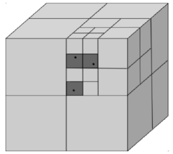
A point cloud can be coded using an octree which is recursively constructed: the root node represents the entire space spanned by all the points, which is equally partitioned along the three dimensions into cubes; the root has eight children, each of which is the root of a sub-octree representing each of the eight cubes. The recursion stops at either an empty cube, or the maximum octree level . Each sub-octree rooted at level represents a cube with side lengths that are of the side lengths of the original space. To code the geometry, the root node records the coordinates of the center of the space, based on which the coordinates of the center of any cube at any level are uniquely determined. Consequently, each non-root node only needs one bit to indicate whether the corresponding cube is empty or not. For the octree in Fig. 1b, the nodes with value at the three levels represent one, two and three non-empty cubes with side lengths of , and in Fig. 1a, respectively. All the non-empty nodes at level collectively represent the geometry information of the point cloud at the spatial granularity of . This makes octree spatially scalable: with one more level of nodes delivered, the spatial resolution doubles (i.e., the distance between points is halved). The color attributes of a point cloud are coded following the octree structure as well, with each node stores the average color attributes of all the points in the corresponding cube. Scalable color coding can be achieved by only coding the difference between a node and its parent. The serialized octree can be further losslessly compressed using entropy coding. With MPEG G-PCC, at each tree level , the status of a node ( or ) is coded using context-based arithmetic coding, which uses a context consisting of its neighboring siblings that have been coded and its neighboring parent nodes to estimate the probability that the node is .
III-B Tile-based Coding and Streaming
Considering the limited viewer Field-of-View (FoV) (dependent on the 6-DoF viewpoint), occlusions between objects and parts of the same object, and the reduced human visual sensitivity at long distances, only a subset of points of a PCV frame are visible and discernible to the viewer at any given time. FoV-adaptive PCV streaming significantly reduces PCV bandwidth consumption by only streaming points visible to the viewer at the spatial granularity that is discernible at the current viewing distance. To support FoV-adaptive streaming, octree nodes are partitioned into slices that are selectively transmitted for FoV adaptability and spatial scalability. Each slice consists of a subset of nodes at one tree level that are independently decodable provided that the slice containing their parents is received. Without considering FoV adaptability, one can simply put all nodes in each tree level into a slice to achieve spatial scalability. The sender will send slices from the top level to the lowest level allowed by the rate budget. To enable FoV adaptability, a popular approach known as tile-based coding is to partition the entire space into non-overlapping 3D tiles and code each tile independently using a separate tile octree. Only tiles falling into the predicted FoV will be transmitted. To enable spatial scalability within a tile, we need to put the nodes at each level of the tile octree into a separate slice. As illustrated in Fig. 1c, each sub-octree rooted at level represents a 3D-tile with side length of . Within each tile sub-octree, nodes down to the level are packaged into a base layer slice, and nodes at the lower layers are packaged into additional enhancement layer slices.
When the streaming server is close to the viewer, one can conduct reactive FoV-adaptive streaming: the client collects and uploads the viewer’s FoV to the server; the server renders the view within the FoV, and streams the rendered view as a 2D video to the viewer. To facilitate seamless interaction and avoid motion sickness, the rendered view has to be delivered with short latency (e.g. 20 ms) after the viewer movement, the so called Motion-to-Photon (MTP) latency constraint [1]. To address the MTP challenge, we consider predictive streaming that predicts the viewer’s FoVs for future frames and prefetches tiles within the predicted FoV [7, 8, 9].
IV Progressive PCV Streaming
Due to the close interaction with PCV objects, viewers are highly sensitive to QoE impairments, such as black screen, freezes, restarts, excessively long latency, etc. Not only the network and viewer dynamics have direct QoE impacts, bandwidth and FoV prediction errors are also critical for the effectiveness of predictive streaming. We propose a novel progressive FoV-adaptive PCV streaming design to minimize the occurrence of the above impairments and deliver a high level of viewer QoE.
IV-A Progressive Downloading/Patching
| Notation | Meaning | |
|---|---|---|
| Download time | ||
| Playback deadline | ||
| Video duration | ||
| Download frequency | ||
| Downloaded rate in round for tile | ||
| Angular resolution | ||
| Level of detail (LoD) | ||
| Tile quality | ||
| Bandwidth constraint | ||
| Maximum rate of tile | ||
| Viewer’s span-in-degree across a tile | ||
| Distance between user viewpoint and tile | ||
| Predicted viewing probability |
Most of the existing FoV-adaptive streaming solutions can be categorized as Sequential-Decision-Making (SDM): at some time point before the playback deadline of a frame, one predicts the viewer FoV at , downloads tiles falling into the predicted FoV at video rates determined by some rate adaptation algorithm, then repeats the process for the next frame. is the time interval for both FoV prediction and frame pre-feteching, which is upper bounded by the client side video buffer length. To achieve smooth streaming, a long pre-fetching interval is preferred to absorb the negative impact of bandwidth variations. However, FoV prediction accuracy decays significantly at long prediction intervals. We have studied the optimal trade-off for setting the buffer length for on-demand streaming of 360o video in [35, 36].
Scalable PCV coding opens up a new dimension to reconcile the conflicting desires for long streaming buffer and short FoV prediction interval. It allows us to progressively download and patch tiles: when a frame’s playback deadline is still far ahead, we only have a rough FoV estimate for it, and will download low resolution slices of tiles overlapping with the predicted FoV; as the deadline approaches, we have more accurate FoV prediction, and will patch the frame by downloading additional enhancement slices for tiles falling into the predicted FoV. Progressive streaming is promising to simultaneously achieve streaming smoothness and robustness against bandwidth variations and FoV prediction errors. On one hand, as shown in Fig. 2, each tile in each segment is downloaded over multiple rounds, the interval of which is . For example, tiles of are downloaded in both round and round . Traditional methods download the segment only once in round based on the FoV prediction at this moment. The benefit of downloading in two rounds is that FoV prediction in round is more accurate than in round . Therefore, the bandwidth can be allocated to the tiles that would be more likely viewed by user. A segment consists of frames with the total video duration of . Within each round, multiple segments are downloaded simultaneously. And the final rendered quality of each tile is a function of the total downloaded rate (thanks to the scalable coding, there is minimal information redundancy between the multiple progressive downloads). The final rendered quality is less vulnerable to network bandwidth variations and the FoV prediction errors at individual time instants. On the other hand, tile downloading and patching are guided by FoV predictions at multiple time instants with accuracy improving over time. If a tile falls into the predicted FoV in multiple rounds, the likelihood that it will fall into the actual FoV is high, and its quality will be reinforced by progressive downloading; if a tile only shows up once in the predicted FoV when its playback time is still far ahead, the chance for it to be in the actual FoV is small. Fortunately, the bandwidth wasted in downloading the low-resolution slices is low.
IV-B Optimal Rate Allocation
Progressive streaming conducts Parallel-Decision-Making (PDM). For a tile in the frame to be rendered at , we prefetch it in the previous rounds, from to . Let denote its download rate in round . The final rate for this tile is . Meanwhile, at download time , all tiles of frames with playback time from to are being downloaded/patched at rates , and the total rate is bounded by the available bandwidth , i.e.,
Suppose is the rendered quality of a tile at rate when viewed from distance , and , are the predicted view likelihood and view distance for tile of frame to be rendered at time . One greedy solution for bandwidth allocation at download time is to maximize the expected quality enhancements for all the active frames, based on the current FoV estimations:
| (1) |
, where is a decreasing function of , considering that FoV estimate accuracy drops for far away frames.

IV-C View-distance based Tile Utility Model
In this section, we explain in detail the proposed tile utility model in Equation (IV-B). Tile quality depends on its angular resolution , which is the number of points per degree that are visible to the user within the tile. There are many subjective studies about the quality of rendered images or videos, but most of them only consider the impact of rate, while very few consider the distance between the viewer and the object, which can be very dynamic in PCV streaming. A subjective study in [8] suggests that users’ QoE changes significantly when they view a rendered point cloud object at different distances. The authors showed a reasonable curve telling the relations between utility, rate and viewing distance. Unfortunately, it didn’t provide a specific utility model. In our work, we try to find a specific tile utility function with respect to viewing distance and tile rate that generates the same trend of curve in [8]. For the traditional 2D video frames/tiles, which is assumed to be viewed from a fixed distance, we can infer the direct mapping from rate to quality, which is usually a logarithm function. However, it is not that clear how the rate and viewing distance simultaneously impact the perceived quality of point cloud tiles. A quality model of image with respect to both distance and resolution was proposed in [37], but it doesn’t directly fit with point cloud video. Nevertheless, it is inspired from [37] that the perceived quality for an object depends on the angular resolution, which depends on the viewing distance and physical size of the object, as well as image resolution. Following [37], we assume that the perceived quality of a viewed tile is logarithmically increasing with the angular resolution , which is the number of points per degree within the tile. With more and more points inside the tile, the per-degree utility increases but more and more slowly. Let be the per-degree quality of a tile, we assume that the perceived quality of a tile that covers degree in either horizontal or vertical direction is
where is a constant factor to be determined by the saturation threshold. As shown in Fig. 3, each tile is a suboctree, and is decided by the level of detail (LoD) which is the suboctree’s height within the tile, and the viewer’s span-in-degree across the tile:
where is the distance between the viewer and the tile, and is the physical side length of a tile. Therefore, the tile utility model is:
| (2) |
where .

To achieve a level of detail (LoD) , all nodes up to level of the tile suboctree has to be delivered, which will incur a certain rate (the total number of bits to code a tile to level ). We have coded several test PCVs using MPEG G-PCC and found that the LoD is logarithmically related to the rate. Due to tile diversity, the data rate needed to code octree nodes up to level is highly tile-dependent. In other words, given a coding rate budget , the achievable LoD is tile-dependent. Let be the rate-LoD mapping for tile within frame , we assume
where the parameters are obtained by fitting the actual rate data for the tiles coded using G-PCC. Substituting this expression into (2) yields:
| (3) |
Note that tile utility is not necessarily at , because there is possibly one point inside the tile. There’s only one parameter to be decided: , which controls the shape of the curve. We decide its value by reasoning that the utility should saturate at some point even if we keep increasing rate and/or distance. This is due to human visual acuity: generally we cannot resolve any two points denser than points per degree [38]. In other words, the derivative of with respect to should be zero given any rate when is so large that the angular resolution reaches :
The derivative goes to zero when is if .
Then we can get the curve similar to the one in [8]. Taking a tile for example, the utility curve with respect to tile rate and distance is shown in Fig. 4. It’s a tile from point cloud video Long Dress of 8i [15], where the figure is high and tile is at the 4th level of the whole octree. For more details about the dataset, please refer to Section V. For simplicity, we ignore the subscripts of as in the following sections.


IV-D Water-filling Rate Allocation Algorithm
We now develop an analytical algorithm for solving the utility maximization problem formulated in Sec. IV-B. In Equation (IV-B), the second term represents the tile quality of the layers that have been downloaded to the buffer before the current round, which is a given constant for the rate optimization at the current round. The utility maximization problem for each round is simplified as below, along with the constraints:
| (4a) | ||||
| subject to | ||||
| (4b) | ||||
| (4c) | ||||
| (4d) | ||||
where is the video length, and is the maximum rate of each tile . The tile rate allocation problem is similar to the typical water-filling problem, where we “fill” the tiles in an optimal order based on their significance determined by the existing rates, probability to be viewed, distance from the viewer, and the calibration weights .
Equation (4) is a nonlinear optimization problem so that the Karush–Kuhn–Tucker (KKT) conditions serve as the first-order necessary conditions. Furthermore, the KKT conditions for this problem are also sufficient due to the fact that the tile utility model is concave in terms of with a given , and the inequality constraints (4b) and (4) are continuously differentiable and convex, and (4d) is an affine function. Therefore, we apply KKT conditions to optimally solve this tile rate allocation problem as shown in Algorithm 1. And the detailed KKT condition-based optimization is explained in Section IV-E.
IV-E KKT Condition-based Optimization
In this section, we explain how to embed KKT condition-based optimization into Problem 4. We follow the standard procedures of KKT conditions.
IV-E1 Standard Formulation
First, we need to simplify the symbols in Problem (4). At each update time , we call this KKT optimization, so we eliminate to simplify the variables: is replaced by , which is the resulting tile rate after this update round. Also, we simplify the constants as , as , and as , where and is tile index within each frame . What’s more, we define , the existing downloaded rate for tile . Problem 4 can be simplified as below:
| (5a) | ||||
| subject to | ||||
| (5b) | ||||
| (5c) | ||||
| (5d) | ||||
Next, we define several functions for different parts of Problem (4). Let , , , and , where r, and are vectors of , and respectively. Then we rewrite the above equations once more into the standard form of KKT condition:
| (6a) | ||||
| subject to | ||||
| (6b) | ||||
| (6c) | ||||
| (6d) | ||||
IV-E2 Analytical Algorithm
The solutions satisfying KKT conditions for this problem are also sufficient because is concave, both and are continuously differentiable and convex, and is affine. We follow the standard steps to solve it. With Lagrange multipliers, (6) is transformed as:
| (7a) | ||||
| (7b) | ||||
Then we derive the properties of the solution based on the following KKT conditions:
Stationarity:
| (8) |
therefore,
where is a constant when is given.
Dual feasibility:
| (9) |
Complementary slackness:
| (10) |
therefore,
Therefore, the optimal rate allocation has three possible solutions according to conditions (8) and (10):
| (11) |
Once is decided, all are decided. Therefore, the goal is to find the optimal . The analytical water filling algorithm for finding is described in Algorithm 2.
IV-E3 Complexity Analysis
From Algorithm 1, at each update time , there are three steps to output the tile rate allocation solution.
-
1.
FoV prediction: We use truncated linear regression with history window size to predict future viewpoints. The regression time in worst case is using sklearn package in Python. The inference time is .
-
2.
Hidden Point Removal (HPR): We use the HPR function in open3d package in Python. The time complexity is using the algorithm in [39], where is maximum number of points in each frame. To make HPR faster, we downsampled the original point cloud to just points per frame before running HPR.
-
3.
KKT-Condition based optimization: Algorithm 2 performs a line search looking for the optimal . The line search takes at least steps in the range . And within each loop we need to obtain the rates for all the tiles within the update window, the complexity of which is where is the number of tiles in a frame that is around on average. Thus, the time complexity of line search is .
However, we actually implement Algorithm 2 using binary search, which is obviously faster than line search. Before binary search, we sort the values which costs . Then, similar to the analysis of line search, the binary search process costs , which has the same complexity as the sorting process.
To sum up, the time complexity at each update time is , where , and . All the variables, , are relatively small, so the algorithm can achieve the update rate of on moderately configured server with Intel(R) Xeon(R) Platinum 8268 CPU @ 2.90GHz.
V Evaluation
In this section, we demonstrate the superiority of the proposed approach over several baselines.
V-A Setup
V-A1 Datasets
We used point cloud videos from the 8i website [40], which includes 4 videos, each with frames with frame rate of fps. The user FoV trace is from [15] which involves participants watching looped frames of the 8i videos on Unity game engine. The bandwidth trace is from NYU Metropolitan Mobile Bandwidth Trace [41], which includes 4G bandwidth traces collected in NYC when traveling on buses, subways, or ferry.
V-A2 Key Parameters
In this section, we show the table of the key parameters used in our experiment.
| Parameter | Value | |
|---|---|---|
| Download frequency | ||
| Update window size | ||
| Segment length | ||
| Frame rate | ||
| number of tile rate versions | ||
| FoV prediction history win | ||
| FoV span | ||
| Bandwidth prediction history win |
We set update window size (buffer length) , which is a relatively long buffer, for unlike the traditional 2-D video, point cloud video is more sensitive to the bandwidth variations due to its higher data rate, so a longer buffer/larger interval is better at handling unstable bandwidth condition. Nowadays, even for 2-D videos, long video buffers are common in Netflix or Youtube VoD streaming. In addition, the larger the interval, the less accurate the FoV prediction. In our case, it’s extremely hard to get accurate FoV prediction for ahead, and that’s why non-progressive method doesn’t work well. Nonetheless, the proposed KKT-based progressive framework performs well even if the interval is as large as , because it progressively downloads every frame over multiple rounds as the frame is moving toward buffer front and FoV prediction becomes more and more accurate. As a result, the proposed progressive framework can achieve smooth streaming with long buffers while dealing well with the FoV prediction errors at a large prediction intervals.
V-A3 FoV Prediction and Bandwidth Prediction
FoV prediction method used in this work is linear regression, while other approaches like neural network based prediction model can also be used in our proposed framework. More specifically, we predict at most future simultaneously using past frames, which is an empirical best history window size reported in [8]. The FoV span is . The prediction accuracy results with different future prediction window sizes are reported in Section V-C1.
We predict future bandwidth by harmonic mean, which is a common and simple bandwidth prediction method. More specifically, it predicts the bandwidth in future one second by calculating the harmonic mean of previous bandwidth within a history window. In our work, we set the history window size to seconds. Since bandwidth prediction is orthogonal to the tile rate allocation algorithm design, we didn’t use more complicated bandwidth prediction methods.
V-B Baselines
-
1.
Non-progressive Downloading: This baseline is similar to the traditional video streaming in 2D video with one new segment downloaded to the end of the streaming buffer in each round. The rate allocation between frames within each new segment is optimized using a KKT algorithm similar to Algorithm 1 and 2, based on just one-time FoV prediction result.
-
2.
Progressive with Equal-allocation: To demonstrate the effectiveness of KKT based optimization approach for progressive streaming, we evaluate a naive progressive streaming baseline where the available bandwidth is equally allocated over all active tiles falling into the predicted FoV at each round.
-
3.
Rate-Utility Maximization Algorithm (RUMA): In the related state-of-the-art work [7], the authors proposed a tile utility model where the tile utility is simply the logarithm of the tile rate multiplied by the number of differentiable points. Based on this model, the authors further proposed a greedy heuristic tile rate allocation algorithm which we call RUMA for short. RUMA didn’t explicitly introduce the concept of scalable PCV coding. Different from RUMA, in our work, we formulate the PCV streaming problem with a well developed concept of scalable coding, and propose a more refined utility model that better reflect viewer’s visual experience when viewing a point cloud tile from certain distance. To achieve this, we have coded several test PCVs using MPEG G-PCC and found that the level of detail (LoD) is logarithmically related to the rate. Due to tile diversity, the data rate needed to code octree nodes up to level is highly tile-dependent. In other words, given a coding rate budget , the achievable LoD is tile-dependent. We fit the coefficients of this logarithmic mapping from rate to LoD, and model the tile utility as a function of the angular resolution to replicate the empirical subjective utility-(rate, distance) curve in [8], which makes our utility model more convincing. Also, we adopt KKT to solve the continuous version of the rate allocation problem then round the rate to its discrete version. We show through simulation experiments that our method outperforms RUMA.
V-C Experimental Results
We run simulations with real users’ FoV traces [15] over four 8i videos. The height of the point cloud cube is and roots of tiles are at level of the whole octree. Each tile subtree has 6 different levels of detail. The update window size is , and it moves forward every one second. We are using FoV traces and bandwidth traces, and the quality results are averaged over frames in Table III and IV.
Table III and IV display mean and variance of different metrics in different scenarios. When both the bandwidth and the FoV oracles are available (Scenario A), non-progressive streaming is comparable with progressive streaming. But in the realistic setting with network bandwidth estimation errors and FoV prediction errors (Scenario B), our proposed progressive streaming solution with either constant or exponentially decreasing frame weights can deliver much higher quality in most cases, measured using both the quality per degree and the delivered angular resolution or the number of points per viewing degree, averaged over all FoV tiles.
| Scen- | Non- | Equal- | RUMA | Progressive KKT | |
| ario | Progressive | Split | Constant | Exp | |
| A | 18.9, 3.0 | 17.3, 1.6 | 19.5, 1.7 | 19.5, 1.6 | N/A |
| B | 6.1, 6.0 | 15.0, 2.0 | 15.9, 2.5 | 15.4, 1.8 | 18.3, 1.9 |
| Scen- | Non- | Equal- | RUMA | Progressive KKT | |
| ario | Progressive | Split | Constant | Exp | |
| A | 5.45, 0.42 | 5.34, 0.39 | 5.49, 0.39 | 5.50, 0.38 | N/A |
| B | 2.50, 1.53 | 5.15, 0.44 | 4.46, 0.63 | 5.16, 0.39 | 5.42, 0.41 |
| Scen- | Non- | Equal- | Progressive KKT | |
|---|---|---|---|---|
| ario | Progressive | Split | Constant | Exp |
| B | 13.49 KB | 6.34 KB | 11.78 KB | 5.19 KB |
We believe that in addition to the average results from Table III and IV, it’s also very important to show the frame quality evolution across time in specific streaming sessions in Fig. 5 and Fig. 6 to demonstrate the drawback of non-progressive baseline as well as the superiority of progressive downloading due to its multi-round downloading with more and more accurate FoV prediction for every frame. In the following sections, we show the comparison results in real-world Scenatio B only. In Section V-C1, we show results for each of the four 8i videos, while the rest of the sections only present the detailed results for Long Dress because all the other videos have similar trends.
V-C1 KKT-const V.S. non-progressive
Quality Supremacy: Only the tiles in the user’s actual FoV are counted into the final quality using Equation (2). Fig. 5a and Fig. 5b as well as Fig. 6 show the frame quality evolution results. A drop around frame index can be observed. The reason is that we assume the server knows the initial 6-DoF viewpoint of the user if he/she starts watching the first frame. Since it’s cold start, the first frames will be downloaded before being watched, so we need to predict FoV for each of the frames and only download the tiles within the predicted FoV. Obviously the predicted 6-DoF viewpoints for the first frames using Linear Regression (LR) would be the same as the initial 6-DoF viewpoint, because there’s only one history data sample which is exactly the initial 6-DoF viewpoint. And it turns out that the constant predicted viewpoint for the first frames is not too bad because the viewer doesn’t move dramatically away from the initial viewpoint. Therefore, the quality of first frames are not bad. However, after the cold start, when the viewer starts watching more frames, the FoV prediction for the following frames (from frame) will be quite different than the initial viewpoint using Linear Regression (LR) because there are more than one history viewpoints in the LR history window now. Since the prediction horizon is as large as future frame ( later), the prediction accuracy would be very bad. Therefore, we observe the drop in the non-progressive curve right after the first frames in the figures. The results mainly demonstrate that the non-progressive framework is super sensitive to FoV prediction error under a long buffer, while the proposed progressive framework can deal with that by progressively downloading every frame for multiple rounds as the frame is moving toward buffer front and FoV prediction becomes more and more accurate.
Except for the first frames where the FoV prediction accuracy for both algorithms is accurate, KKT-const, which uses constant weights for all frames in KKT calculation, dominates non-progressive baseline in terms of both angular resolution and per-degree quality by a large gap on average. The reason is that the non-progressive baseline predicts FoV for every frame 20 seconds ahead and download the tiles only once based on the predicted FoV, which is absolutely not accurate due to the large prediction interval. Therefore, several frames have almost zero angular resolution and pretty low per-degree quality in this case. In contrast, by progressive downloading, KKT-const predicts FoV and improves the tiles’ rates for every frame over rounds, with the prediction accuracy becomes more and more accurate over time.
Smoothness: In Fig. 5a, 5b and 6, The large quality variation suffered by nonprogressive baseline is also due to the bandwidth variations. At each downloading round of non-progressive baseline, we allocate all the predicted available bandwidth to just one segment consisting of frames that are about to enter the end of buffer. In contrast, at each downloading round of KKT-const, it updates all the frames in the buffer simultaneously based on the optimization algorithm, which smooths the resulting frame quality evolution dramatically.


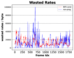


Bandwidth Consumption: At each downloading time of KKT-const, for the frames farther away from playing, e.g., 20s ahead, since the FoV prediction is not so accurate we just download a base layer for the tiles within the predicted FoV, which doesn’t waste too much bandwidth; while for the frames closer to user playback time, we patch the tiles within the more accurately predicted FoV by downloading additional enhancement layers. However, non-progressive baseline allocates all the bandwidth to just one segment based on inaccurate FoV prediction. Therefore, in both Table V and Fig. 5c we observe that KKT-const helps save a lot of bandwidth over all the frames. The bandwidth wastage savings would be significant for long PCVs. What is worth mentioning is that in Fig. 5c, we want to fairly compare the wasted rates due to FoV prediction errors between the non-progressive framework and our progressive algorithm. The x-axis extends to instead of , because we remove the comparison results for the first frames. The FoV prediction for the first frames are always good as explained in Section V-C1, so the wasted rates of both algorithms are very small for the first frames. Therefore, we remove them so that the results of the rest frames look more clear.


| Metrics | KKT-exp | RUMA | Equal- | Non- |
| Split | Progressive | |||
| PSNR | 43.05 | 42.89 | 42.76 | 41.88 |
| SSIM | 0.9725 | 0.9695 | 0.9691 | 0.9610 |
Correlation between Quality Improvement and FoV prediction Accuracy: To verify the motivation of progressive streaming, we zoom in to see the correlation between the quality improvements of progressive streaming and the FoV prediction accuracy. The FoV prediction accuracy in terms of Mean Absolute Error (MAE) with respect to future window sizes (at most frames ahead) for 6 DoF is shown in Fig. 8. In the progressive downloading process, each frame’s FoV is predicted for times in a 600-frame update window. In Fig. 9a, we show the FoV prediction accuracy in terms of tile overlap ratio with ground-truth user FoV for each frame, where a larger overlap ratio means a more accurate prediction. The blue curve is the first-time prediction when the frame is just download into the buffer and far away from playback time; the red curve is the last-time prediction when the frame is closest to playback time; and black curve is the average accuracy over predictions. The difference between red and blue curves in Fig. 9a represents the FoV prediction accuracy difference between the front and end position in the buffer. We also calculate the quality improvement between KKT-const and non-progressive baseline. When we put the two difference curves together in Fig. 9b, we find an obvious correlation between the two: if the FoV prediction at the front of the buffer (closer to user playback time) is much better than that at the end of buffer (way ahead of user playback time), the quality improvement of progressive-const against the non-progressive is much larger. The pattern is more obvious in the scatter-plot in Fig. 9c. The correlation coefficient is .
V-C2 KKT-exp V.S. KKT-const
We further explore the design space of setting frame weights in Equation (4a). The frame weights depend on the confidence about the accuracy of FoV prediction for each frame. Therefore, intuitively, it should decrease as the prediction interval increases. We tried several different weight settings, including linear decreasing, history FoV prediction accuracy based assignment, and exponentially decreasing in terms of prediction interval. We found the exponentially decreasing frame weights performs the best, as shown in Table III, IV and V, as well as in Fig. 10a and 10b KKT-exp further boosts the per-degree frame quality on top of KKT-const without increasing too much quality variations. From Fig. 10a and Table V we see a large amount of bandwidth is further saved by KKT-exp.
In Fig. 10a, we can see for some frames the visible rates (i.e. the bits used inside the actual FoV) is more than doubled. That is because the long-term FoV prediction accuracy is low, and downloading tiles outside the actual FoV wastes a lot of bandwidth. We randomly pick some of these frames as an example to zoom in the improvements of tile quality in different scenarios. We show the improvement distribution over visible tiles in different network conditions, also with different FoV traces that have different distances between the user and the object, since those are two important factors affecting the final viewing quality.


Fig. 11a, 11b and 11c show the CDF of tile rate, resolution and quality improvement respectively under different network conditions and user-object distances. Resolution is the number of points per degree along one dimension in every tile. When bandwidth is high () and distance is normal () (red curves), the average visible frame rate of KKT-const is KB, KKT-exp is KB, times of KKT-const. On average, the resolution of KKT-const is pts / degree, while KKT-exp is pts / deg, improved by . Also, the average tile quality for KKT-const is 28, while KKT-exp is 31, improved by . Although the tiles rate difference is pretty large in this case (red curve) in Fig. 11a, the resolution difference may not be that large because some tiles have higher compression efficiency than others, or they have fewer points.
When bandwidth is small () and distance is normal () (blue curves), the average visible frame rate of KKT-const is Bytes, KKT-exp is Bytes, times of KKT-const. The average resolution in this case is for KKT-const and for KKT-exp. Also, the average tile quality for KKT-const is 19, while KKT-exp is 23, improved by . Compared to the previous scenario where bandwidth is ten times larger, the tile quality now appears more sensitive to the tile rate. Therefore, although the tile rate improvement ratio is not as large as the previous scenario when bandwidth is high, the tile quality improvement ratio is similar.
We further demonstrate that tile quality is more sensitive to user-object distance change. We keep the bandwidth at a medium level (), while selecting a FoV trace for which the average user-object distance is only m. Now the average frame rate improvement is times larger. The resolution improvement is even smaller: for KKT-const and for KKT-exp. The absolute difference is only less than 2 pts / degree. However, the mean tile quality improvement is the largest among all scenarios as observed from the green curve in Fig. 11c, for which the absolute improvement of KKT-exp compared to KKT-const is . This result demonstrates that the tile quality is most sensitive to tile rate when user-object distance is small. Therefore, KKT-exp has the greatest improvement compared to KKT-const when the user watches the point cloud object very closely.
V-C3 KKT-exp V.S. Equal Allocation
To demonstrate the superiority of KKT-based tile rate allocation for PCV streaming, we design an equal allocation baseline, where the predicted available bandwidth is equally split over all the tiles within the predicted FoV of every frame. We show the angular resolution per frame comparison to the equal allocation baseline in Fig. 12a, and resolution improvement CDF distribution in Fig 12b, where KKT-exp reaches against of Equal allocation. Additionally, we show mean tile quality improvement CDF in Fig. 12c.


V-C4 KKT-exp V.S. RUMA
We now compare KKT-exp with the state-of-the-art rate allocation algorithm RUMA [7]. In Fig. 13a, we see the per-degree frame quality evolution over time. The mean per-degree quality of KKT-exp is against of RUMA, an improvement by on average.


In Fig. 13b, we zoom in some frames whose quality improvement is larger than the others. We can see that due to the greediness of RUMA, even if some tiles have achieved the highest quality, it fails to optimize the rate allocation that should consider all the tiles of interests. Also, the intermediate steps of RUMA estimate the marginal tile utility by finite difference, which is not accurate enough to ensure an optimal solution. Instead, we first use KKT to solve the continuous rate allocation problem, which guarantees the optimality because we use the true marginal utility in the calculation. We then round the solution to each tile’s discrete rate version.
V-C5 Visual Results
In Fig. 7, we show the example reandered views of different baselines. The artifacts of “Equal Split” and “Non-Progressive” can be easily observed. Non-progressive result looks weird because it downloads each frame only once when the the frame is about to be download into buffer and the FoV prediction is very inaccurate. For state-of-art “RUMA”, when we zoom in we can see the obvious artifacts around hair, right face and chest as well as left thigh, while there’s no obvious artifacts for “KKT-exp”. We also show the average PSNR and SSIM results in Table VI. We conclude that the proposed KKT-Condition based progressive downloading strategy performs better than the baselines in terms of visual results, which proves the rationality of the proposed quality model.
VI Acknowledgements
The project was partially supported by USA National Science Foundation under award number CNS-2312839.
VII Conclusion
As volumetric video is on the rise, we explore the design space of point cloud video streaming which is challenging due to its high communication and computation requirements. By relying on the inherent scalability of octree-based point cloud coding, we proposed a novel sliding-window based progressive streaming framework to gradually refine the spatial resolution of each tile as its playback time approaches and FoV prediction accuracy improves. In this way, we managed to balance needs of long streaming buffer for absorbing bandwidth variations and short streaming buffer for accurate FoV prediction. We developed an analytically optimal algorithm based on the Karush–Kuhn–Tucker (KKT) conditions to solve the tile rate allocation problem. We also proposed a novel tile rate-utility model that explicitly considers the viewing distance to better reflect the true user QoE. In the future, we will not only consider maximizing the total tile utility, but also controlling the quality variations between consecutive frames, which leads to a more complicated non-concave objective function, and introduces stronger coupling between rate allocations on adjacent frames. We will apply nonlinear optimal control techniques, e.g. iterative Linear Quadratic Regulator (iLQR), to solve the optimal rate allocation problem.
References
- [1] E. Cuervo, K. Chintalapudi, and M. Kotaru, “Creating the perfect illusion: What will it take to create life-like virtual reality headsets?” in Proceedings of the 19th International Workshop on Mobile Computing Systems & Applications, 2018, pp. 7–12.
- [2] S. Akhshabi, A. C. Begen, and C. Dovrolis, “An experimental evaluation of rate-adaptation algorithms in adaptive streaming over http,” in Proceedings of the second annual ACM conference on Multimedia systems, 2011, pp. 157–168.
- [3] R. Chen, M. Xiao, D. Yu, G. Zhang, and Y. Liu, “patchvvc: A real-time compression framework for streaming volumetric videos,” in Proceedings of the 14th Conference on ACM Multimedia Systems, 2023, pp. 119–129.
- [4] S. Wang, M. Zhu, N. Li, M. Xiao, and Y. Liu, “Vqba: Visual-quality-driven bit allocation for low-latency point cloud streaming,” in Proceedings of the 31st ACM International Conference on Multimedia, 2023, pp. 9143–9151.
- [5] J. Zhang, T. Chen, D. Ding, and Z. Ma, “G-pcc++: Enhanced geometry-based point cloud compression,” in Proceedings of the 31st ACM International Conference on Multimedia, 2023, pp. 1352–1363.
- [6] Y. Wang, D. Zhao, H. Zhang, C. Huang, T. Gao, Z. Guo, L. Pang, and H. Ma, “Hermes: Leveraging implicit inter-frame correlation for bandwidth-efficient mobile volumetric video streaming,” in Proceedings of the 31st ACM International Conference on Multimedia, 2023, pp. 9185–9193.
- [7] J. Park, P. A. Chou, and J.-N. Hwang, “Rate-utility optimized streaming of volumetric media for augmented reality,” IEEE Journal on Emerging and Selected Topics in Circuits and Systems, vol. 9, no. 1, pp. 149–162, 2019.
- [8] B. Han, Y. Liu, and F. Qian, “Vivo: Visibility-aware mobile volumetric video streaming,” in Proceedings of the 26th annual international conference on mobile computing and networking, 2020, pp. 1–13.
- [9] K. Lee, J. Yi, Y. Lee, S. Choi, and Y. M. Kim, “Groot: A real-time streaming system of high-fidelity volumetric videos,” in Proceedings of the 26th Annual International Conference on Mobile Computing and Networking, ser. MobiCom ’20. New York, NY, USA: Association for Computing Machinery, 2020. [Online]. Available: https://doi.org/10.1145/3372224.3419214
- [10] A. Zhang, C. Wang, B. Han, and F. Qian, “YuZu: Neural-Enhanced Volumetric Video Streaming,” in 19th USENIX Symposium on Networked Systems Design and Implementation (NSDI 22), 2022, pp. 137–154.
- [11] Y. Liu, B. Han, F. Qian, A. Narayanan, and Z.-L. Zhang, “Vues: practical mobile volumetric video streaming through multiview transcoding,” in Proceedings of the 28th Annual International Conference on Mobile Computing And Networking, 2022, pp. 514–527.
- [12] L. Wang, C. Li, W. Dai, J. Zou, and H. Xiong, “Qoe-driven and tile-based adaptive streaming for point clouds,” in ICASSP 2021-2021 IEEE International Conference on Acoustics, Speech and Signal Processing (ICASSP). IEEE, 2021, pp. 1930–1934.
- [13] L. Wang, C. Li, W. Dai, S. Li, J. Zou, and H. Xiong, “Qoe-driven adaptive streaming for point clouds,” IEEE Transactions on Multimedia, 2022.
- [14] S. Rossi, I. Viola, L. Toni, and P. Cesar, “Extending 3-dof metrics to model user behaviour similarity in 6-dof immersive applications,” in Proceedings of the 14th Conference on ACM Multimedia Systems, 2023, pp. 39–50.
- [15] S. Subramanyam, I. Viola, A. Hanjalic, and P. Cesar, “User centered adaptive streaming of dynamic point clouds with low complexity tiling,” in Proceedings of the 28th ACM international conference on multimedia, 2020, pp. 3669–3677.
- [16] J. Kammerl, N. Blodow, R. B. Rusu, S. Gedikli, M. Beetz, and E. Steinbach, “Real-time compression of point cloud streams,” in 2012 IEEE international conference on robotics and automation. IEEE, 2012, pp. 778–785.
- [17] Y. Shi, P. Venkatram, Y. Ding, and W. T. Ooi, “Enabling low bit-rate mpeg v-pcc-encoded volumetric video streaming with 3d sub-sampling,” in Proceedings of the 14th Conference on ACM Multimedia Systems, 2023, pp. 108–118.
- [18] R. Mekuria, K. Blom, and P. Cesar, “Design, implementation, and evaluation of a point cloud codec for tele-immersive video,” IEEE Transactions on Circuits and Systems for Video Technology, vol. 27, no. 4, pp. 828–842, 2016.
- [19] A. Zhang, C. Wang, B. Han, and F. Qian, “Efficient volumetric video streaming through super resolution,” in Proceedings of the 22nd International Workshop on Mobile Computing Systems and Applications, 2021, pp. 106–111.
- [20] X. Sheng, L. Li, D. Liu, Z. Xiong, Z. Li, and F. Wu, “Deep-pcac: An end-to-end deep lossy compression framework for point cloud attributes,” IEEE Transactions on Multimedia, vol. 24, pp. 2617–2632, 2021.
- [21] J. Wang, H. Zhu, H. Liu, and Z. Ma, “Lossy point cloud geometry compression via end-to-end learning,” IEEE Transactions on Circuits and Systems for Video Technology, vol. 31, no. 12, pp. 4909–4923, 2021.
- [22] Y. Mao, Y. Hu, and Y. Wang, “Learning to predict on octree for scalable point cloud geometry coding,” in 2022 IEEE 5th International Conference on Multimedia Information Processing and Retrieval (MIPR). IEEE, 2022, pp. 96–102.
- [23] Z. Liu, J. Li, X. Chen, C. Wu, S. Ishihara, and Y. Ji, “Fuzzy logic-based adaptive point cloud video streaming,” IEEE Open Journal of the Computer Society, vol. 1, pp. 121–130, 2020.
- [24] J. Van Der Hooft, T. Wauters, F. De Turck, C. Timmerer, and H. Hellwagner, “Towards 6dof http adaptive streaming through point cloud compression,” in Proceedings of the 27th ACM International Conference on Multimedia, 2019, pp. 2405–2413.
- [25] Y. Gao, P. Zhou, Z. Liu, B. Han, and P. Hui, “Fras: Federated reinforcement learning empowered adaptive point cloud video streaming,” arXiv preprint arXiv:2207.07394, 2022.
- [26] J. Li, C. Zhang, Z. Liu, R. Hong, and H. Hu, “Optimal volumetric video streaming with hybrid saliency based tiling,” IEEE Transactions on Multimedia, 2022.
- [27] J. Li, H. Wang, Z. Liu, P. Zhou, X. Chen, Q. Li, and R. Hong, “Towards optimal real-time volumetric video streaming: A rolling optimization and deep reinforcement learning based approach,” IEEE Transactions on Circuits and Systems for Video Technology, 2023.
- [28] M. Rudolph, S. Schneegass, and A. Rizk, “Rabbit: Live transcoding of v-pcc point cloud streams,” in Proceedings of the 14th Conference on ACM Multimedia Systems, 2023, pp. 97–107.
- [29] J. Zhang, T. Chen, D. Ding, and Z. Ma, “Yoga: Yet another geometry-based point cloud compressor,” in Proceedings of the 31st ACM International Conference on Multimedia, 2023, pp. 9070–9081.
- [30] D. Graziosi, O. Nakagami, S. Kuma, A. Zaghetto, T. Suzuki, and A. Tabatabai, “An overview of ongoing point cloud compression standardization activities: Video-based (v-pcc) and geometry-based (g-pcc),” APSIPA Transactions on Signal and Information Processing, vol. 9, 2020.
- [31] Google. (2017) Draco 3d data compression. [Online]. Available: https://google.github.io/draco/
- [32] M. Hosseini and C. Timmerer, “Dynamic adaptive point cloud streaming,” in Proceedings of the 23rd Packet Video Workshop, 2018, pp. 25–30.
- [33] A. Ak, E. Zerman, M. Quach, A. Chetouani, A. Smolic, G. Valenzise, and P. Le Callet, “Basics: Broad quality assessment of static point clouds in a compression scenario,” IEEE Transactions on Multimedia, 2024.
- [34] A. Ak, E. Zerman, M. Quach, A. Chetouani, G. Valenzise, and P. Le Callet, “A toolkit to benchmark point cloud quality metrics with multi-track evaluation criteria,” in 2024 IEEE International Conference on Image Processing (ICIP 2024), 2024.
- [35] L. Sun, F. Duanmu, Y. Liu, Y. Wang, Y. Ye, H. Shi, and D. Dai, “Multi-path multi-tier 360-degree video streaming in 5g networks,” in Proceedings of the ACM Multimedia Systems Conference, 2018.
- [36] ——, “A two-tier system for on-demand streaming of 360 degree video over dynamic networks,” IEEE Journal on Emerging and Selected Topics in Circuits and Systems, vol. 9, no. 1, pp. 43–57, 2019.
- [37] J. H. Westerink and J. A. Roufs, “Subjective image quality as a function of viewing distance, resolution, and picture size,” SMPTE journal, vol. 98, no. 2, pp. 113–119, 1989.
- [38] wikipedia, “visual acuity,” 2023. [Online]. Available: https://en.wikipedia.org/wiki/Visual_acuity
- [39] S. Katz, A. Tal, and R. Basri, “Direct visibility of point sets,” in ACM SIGGRAPH 2007 papers, 2007, pp. 24–es.
- [40] E. d’Eon, B. Harrison, T. Myers, and P. A. Chou, “8i voxelized full bodies-a voxelized point cloud dataset,” ISO/IEC JTC1/SC29 Joint WG11/WG1 (MPEG/JPEG) input document WG11M40059/WG1M74006, vol. 7, no. 8, p. 11, 2017.
- [41] L. Mei, R. Hu, H. Cao, Y. Liu, Z. Han, F. Li, and J. Li, “Realtime mobile bandwidth prediction using lstm neural network,” in Passive and Active Measurement: 20th International Conference, PAM 2019, Puerto Varas, Chile, March 27–29, 2019, Proceedings 20. Springer, 2019, pp. 34–47.