Progress in Higgs inflation

As inflation has been regarded as a standard paradigm describing the early universe, it also has become important to understanding how inflation is actually realized in particle physics models. In the Standard Model(SM), there is an unique candidate, which is the Higgs boson.

Unfortunately, the chaotic inflation type of potential $V\propto\phi^{n}$ is known to be inconsistent with cosmological measurements because it predicts a large tensor-to-scalar ratio $r$ . However, an additional non-minimal coupling between the Higgs scalar $\phi$ and the Ricci scalar $R$ in the gravity sector flattens the potential in the large field regime in the Einstein frame and suppresses $r$ Bezrukov and Shaposhnikov (2008).

The Lagrangian for the relevant inflaton and gravity sectors is

where $V_{J}(\phi)=\frac{\lambda}{4}(\phi^{2}-v_{\rm EW}^{2})^{2}$ with $v_{\rm EW}\simeq 246~{}\rm GeV$ and $J$ stands for the Jordan frame. To eliminate the non-minimal coupling, we redefine the metric as

where

and we canonicalize the kinetic term with the relation

Then, the action in the canonical Einstein frame is ²²2In fact, the form of the action is different when the Palatini formalism is used, which regard the metrics and affine connection independently. In this review, we take the standard metric formalism.

where

Approximately, the potential takes the form

Note that we neglected $v_{\rm EW}\ll M_{P}/\xi$ and that the potential becomes asymptotically constant at large field values. The e-folding number $N_{e}\equiv\ln a(t_{\rm end})/a(t_{*})$, with ‘end’ meaning the time at the end of the inflation and $*$ meaning CMB pivot scale/time, is

Here, we use $-3H\dot{h}\simeq V^{\prime}(h)$ during slow-roll inflation and $\phi_{*}\gg\phi_{\rm end}$. Normally, the number of e-foldings required to solve the horizon and flatness problems is assumed to be $N\simeq 50-60$.

From the potential in the Einstein frame, we can calculate the slow roll parameters as

where ${\prime}$ denotes the derivative with respect to $h$.

By parameterizing the scalar and tensor power spectrum as

respectively, cosmological observables such as the spectral index and the tensor-to-scalar ratio are approximated with the slow-roll parameters:

which are perfectly consistent with current Planck 2018 measurement Akrami et al. (2018). To satisfy the amplitude of the curvature power spectrum $\log(10^{10}A_{s})=3.047\pm 0.014$, one needs other constraints for $\xi$ and $\lambda$.

Therefore, by assuming $\lambda=0.15$, for example, we have to assume very large non-minimal coupling $\xi\simeq 18000$. Such a large non-minimal coupling causes theoretical issues including naturalness, and more seriously, the unitarity problem Barbon and Espinosa (2009); Burgess et al. (2009, 2010); Lerner and McDonald (2010). We will come back to this issue later in this review.

Note that we assumed constant $\lambda$ and $\xi$ without considering the quantum corrections. In the Higgs inflation case, however, quantum corrections give non-trivial modifications not only to the inflaton dynamics, but also to cosmological observables.

For the currently known Higgs masses and top quark masses, the EW Higgs potential is known to be metastable as $\lambda$ becomes negative when the renormalization scale is $\mu\gtrsim\mathcal{O}(10^{10}\rm GeV)$ Degrassi et al. (2012). This fact may not be a big problem as long as the lifetime of the EW vacuum is longer than the age of the universe. However, if this is the case, the validity of the Higgs inflation scenario may be questioned Bezrukov et al. (2015). ³³3Even in non-Higgs inflation cases, large quantum fluctuation in de Sitter bachground $\mathcal{O}(H/2\pi)$ during inflation may cause a problem. See the Ref. Markkanen et al. (2018a).

However, this result sensitively depends on the top quark mass measurement. In fact, the usually referred to top quark mass is the so-called ‘Monte-Carlo (MC) mass’. This is a mere parameter in MC simulations and the theoretical uncertainties on being identifed as the pole mass are large, up to $\mathcal{O}(1\rm GeV)$ Corcella (2019). Instead, by taking the latest pole mass from cross-section measurements Zyla et al. (2020)

the top quark mass which guarantees the Higgs potential stability $m_{t}^{\rm pole}\lesssim 171.4{\rm GeV}$ is within the $2\sigma$ bound. In this review, we will assume absolute stability of the Higgs potential.

On the other hand, considering the effects of the running of the coupling to Higgs inflation cases is still important Hamada et al. (2014); Bezrukov and Shaposhnikov (2014); Hamada et al. (2015). The quartic coupling can be parameterized as

with $\beta_{2}^{\text{SM}}\approx 0.5$, $\mu_{\text{min}}=\phi_{\text{min}}\sim 10^{17}-10^{18}\,\,\text{GeV}$ as denoted in Degrassi et al. (2012); Buttazzo et al. (2013).⁴⁴4In fact, due to the non-renormalizability of the theory, there exists a dependence on the way to choose the renormalization scale, which is also called ‘prescription’. In this review, we choose $\mu=\phi$, where $\phi$ is the Jordan frame Higgs field value. For the meaning of the prescription dependence in detail, see Ref. Hamada et al. (2017).

One of the major consequences is that small non-minimal couplings, $\xi\gtrsim\mathcal{O}(10)$, are allowed, assuming $\lambda_{*}\sim\mathcal{O}(10^{-3})$. Another possible result is that the form of the potential could have an inflection point when the values of $\lambda$ are tuned to be nearly zero, and this type of inflation is referred to as ‘critical Higgs inflation (CHI)’. This fact has motivated efforts to look into the possibilities of generating primordial black holes (PBH) on the model, as the inflection shape potential is a well-known class of models to induce large curvature power spectrum on small scales producing a significant amount of PBHs.

One should be careful when dealing with the cut-off scale of the Higgs inflation due to the existence of large non-minimal coupling Burgess et al. (2009, 2010); Barbon and Espinosa (2009).

For the small field region $\phi<M_{P}/\xi$, from Eq. (5), fields in each frames are related by

This means that the kinetic term of the field $h$ in the Einstein frame contains derivative couplings

From the second term, one concludes that the theory becomes strongly coupled at $E\gtrsim\Lambda\equiv M/\xi$.

During inflation, the fluctuation is defined with respect to the classical background field value (denoted with ‘bar’) as

Therefore, in the region where $\bar{\phi}>M_{P}/\sqrt{\xi}$ corresponding to the inflationary region,

implying

Therefore, the cut-off scale during inflation is safely higher than the energy scale of inflation Bezrukov et al. (2011).

However, after inflation, the inflaton rolls down to the minimum of the potential and starts to oscillate coherently. Lastly, the Higgs field decays to SM particles and loses its energy. These procedures are called ‘reheating’. During the reheating phase, the decay of the longitudinal gauge boson is violent and the momentum of the produced particles is $k\simeq\mathcal{O}(\sqrt{\lambda}M_{P})$, which is larger than the cut-off scale during the reheating, $M_{P}/\xi$ ⁵⁵5In fact, the Higgs boson decay to the longitudinal mode of the gauge boson may depend sensitively on higher order operators. See the Ref. Hamada et al. (2020). Ema et al. (2017). Above the cut-off scale, decay processes violate unitarity, becoming strongly coupled, and lose its predictivity.

To unitarize the Higgs inflation during reheating, there has been a lot of attempts to raise the cut-off scale of the Higgs inflation by introducing additional degrees of freedom Giudice and Lee (2011); Barbon et al. (2015); Giudice and Lee (2014). One of the simplest and minimal ways is to consider the $R^{2}$ corrections Ema (2017); Gorbunov and Tokareva (2019); He et al. (2019, 2018); Gundhi and Steinwachs (2018), as described in the next section.

The Higgs-$R^{2}$ inflation is a simple UV extension that cures the theoretical/phenomenological issues of single-field Higgs inflation Ema (2017); Gorbunov and Tokareva (2019). The action takes the following form.

where $M$ is the scalaron mass, $h$ is a scalar that stands for the Standard Model Higgs in the unitary gauge, and a conveniently defined function $F(h,R_{J})$ and its derivative with respect to $R_{J}$

The scalaron field $s$ is defined as

Through a Weyl transformation, $g_{\mu\nu}=e^{\omega(s)}g^{J}_{\mu\nu}$, we can get the action in the Einstein frame as

where the scalar potential is

As noted in the potential Eq. (29), higher order operators are induced in the analysis; therefore, the perturbativity of the system is guaranteed for a specific cutoff scale. Expanding the potential around $s\simeq h\simeq 0$ yields a cutoff scale

for scalaron masses within the following range $M\mathrel{\hbox to0.0pt{\lower 4.0pt\hbox{\hskip 1.0pt$\sim$}\hss}\raise 1.0pt\hbox{$<$}}M_{P}/\xi$. This cutoff scale guarantees the perturbative analysis of this model throughout inflation and preheating, alleviating the unitarity problem of single-field Higgs inflation Gorbunov and Tokareva (2019); He et al. (2019, 2018); Gundhi and Steinwachs (2018) .

This additional $R^{2}$ term can also be induced through quantum loop corrections in the large-$\xi$ limit. Renormalization group equations of the system imply a new scalar degree at the mass scale $M\sim M_{P}/\xi$, which in turn corresponds to the strong coupling scale of Higgs inflation Salvio and Mazumdar (2015); Calmet and Kuntz (2016); Wang and Wang (2017); Ema (2017); Ghilencea (2018); Ema (2019); Canko et al. (2019); Ema et al. (2020). Therefore, the addition of the $R^{2}$ term is a natural aspect in terms of both perturbative unitarity and renormalizability.

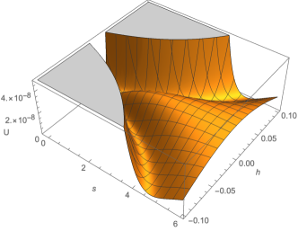
The additional scalar degree of freedom in the action yields a multifield inflationary potential. For a non-critical case with $\lambda=0.01$, the potential takes a valley form as in Fig. 1. Re-formulating the action, we obtain the equation of motion

with

where $G_{ab}$ is the curved field space metric, $D_{a}\phi^{b}=\partial_{a}\phi^{b}+\Gamma^{b}_{ca}\phi^{c}$, $\Gamma^{b}_{ca}=\frac{1}{2}G^{be}\left(\partial_{c}G_{ae}+\partial_{a}G_{ec}-\partial_{e}G_{ca}\right)$, and $D_{t}=\dot{\phi}^{a}\nabla_{a}$. The inflaton will approximately roll down the valley, resulting in successful slow-roll inflation. This particular valley structure exhibits an isocurvature mass $m_{\text{iso}}^{2}\gg H^{2}$, leading to exponentially decaying isocurvature perturbations and allowing for an effective single-field description of the system. The potential along the $h$ direction is locally minimized at

Inserting this into the potential and taking the large $s$ limit, we find that the inflationary potential at the plateau becomes

yielding the cross-correlation between parameters $\lambda,\xi$, and $M$.

After the inflationary stage, the inflaton rolls down to the minimum at $(s,h)\simeq(0,0)$. Depending on the parameters, the inflaton oscillates in both the $s$ and the $h$ directions, making the effective single-field analysis insufficient. In this period, the quantum creation of the NG boson mode from $\mathcal{H}(x)=h(t)e^{i\theta(x)}/\sqrt{2}$ is important. This $\theta$ direction arises from the following terms in the Lagrangian He et al. (2019):

where $\theta_{c}(x)\equiv a^{3/2}(t)e^{-\omega(s)/2}h(t)\theta(x)\equiv F(t)\theta(x)$ and $a$ is the scale factor in the FRW metric. By computing the effective NG mode mass, the peak value takes the form

with $C_{m}\approx 0.25$ and $M_{c}\approx 1.3\times 10^{-5}M_{P}$. This quantity is noticeably lower than the cutoff scale of the theory. Therefore, the violent preheating behavior is present and physical, albeit it is not as violent as it would be in the single field Higgs inflation case and does not violate the unitarity problem Ema et al. (2017).

For specific parameters, the inflaton may climb up the hill of the potential at $h=0$, giving a negative $m_{h}^{2}=-3\omega(s)\xi M^{2}$ and inducing a tachyonic preheating phase Bezrukov et al. (2019); He et al. (2020); Bezrukov and Shepherd (2020). This in turn gives an exponential enhancement to the particle production, rapidly completing the preheating process. The criticality of the Standard Model Higgs quartic coupling may also lead to interesting and unique phenomena in the preheating procedure. We will do a detailed analysis in future works.

In this subsection, we briefly summarize the formulas to obtain the PBH mass spectrum given a curvature power spectrum from inflation.

When the energy density perturbation $\delta\sim\delta\rho/\rho$ ⁶⁶6At linear order, there is a simple relation between the energy density fluctuation and the curvature perturbation: $\displaystyle\delta=\frac{4}{9}\left(\frac{k}{aH}\right)^{2}\mathcal{R}.$ (38) exceeds a critical values $\delta_{c}\simeq 0.3-0.5$ Green et al. (2004); Harada et al. (2013); Musco (2019), the matter in the Hubble sphere with radius $1/H$ starts to collapes to a black hole when the corresponding mode re-enters to the horizon during the radiation dominated (RD) era Carr (1975); Carr et al. (2010). The energy density of the background is also determined by the Hubble parameter. Therefore, the mass of the primordial black hole is determined solely by the Hubble scale at the time of its formation Green et al. (2004),

where $\gamma\simeq 0.2$ represents the efficiency of the collapsing processes and $k=aH$ is the comoving momentum scale on which the primordial black hole is generated. The variance of the density contrast $\sigma\equiv\sqrt{\langle\delta^{2}\rangle}$ is calculated from the curvature power spectrum $\mathcal{P}_{\mathcal{R}}(k)$ and the window function $W(R,k)=\exp(-k^{2}R^{2}/2)$ smoothing over the comoving scale $R\simeq 1/aH|_{\rm form}$:

We follow the ‘peaks theory’ method Green et al. (2004); Young et al. (2014) to compute the PBH abundance and the mass spectrum. We use the variable $\nu_{c}\equiv\delta_{c}/\sigma$. The energy density fraction of PBHs at formation, denoted by $\beta_{M_{\rm PBH}}$ can be calculated using

with

Finally, the fraction of PBHs against the total dark matter energy density is

where $g_{*}=106.75$ is the effective relativistic degree of freedom at the time of formation.

As a minimal extension of Higgs inflation, it is highly motivated to consider the role of the $R^{2}$ term with criticality of the self quartic coupling in generating PBHs as dark matter.

In the Higgs-$R^{2}$ model, three relevant running parameters $(M,\xi,\lambda)$ exist. The 1-loop beta functions are Codello and Jain (2016); Markkanen et al. (2018b); Gorbunov and Tokareva (2019); Ema (2019)

where $\alpha={M_{P}^{2}}/{12M^{2}}$. $\beta_{\rm SM}$ stands for the other terms from the SM De Simone et al. (2009). Among those, as in the original critical Higgs inflation case, the running of $\lambda$ is most important in our analysis.

During inflation, including the inflection point, the Higgs field value is comparable to the Planck scale $h\gtrsim\mathcal{O}\left(0.1M_{P}\right)$. On the other hand, the effects of the Ricci scalar $R=12H^{2}$ in the de Sitter background on determining the renormalization scale is negligible due to the small Hubble parameter $H\sim 10^{-5}M_{P}$. Therefore, we choose our prescription $\mu=h$ and express $\lambda\left(\mu\right)$ as Eq. (17). Note that the Higgs field values are independent of the frame used for Higgs-$R^{2}$ inflation.

The field values $(s,h)=(s^{*},h^{*})$ and the corresponding value $\lambda_{\text{min}}^{\text{inf}}$ for the potential to have an inflection point can be determined by using the conditions

We then compute the $\lambda_{\text{min}}$ value⁷⁷7In fact, to generate a large enough power spectrum, $\lambda_{\text{min}}=\lambda_{\text{min}}^{\text{inf}}-\delta c$, with $\delta c\sim\mathcal{O}\left(10^{-7}\right)$ at the corresponding scale, the $\lambda_{\rm min}$ must be smaller than the pure inflection value $\lambda_{\rm min}$ by as much as $\mathcal{O}(10^{-7})$ so that the potential should deviate from a true inflection point., which we assumed to include all the information from the SM parameters.

Fig. 2 shows the new possibility of the Higgs-$R^{2}$ inflation model generating a sufficient number of PBHs with $f_{\rm PBH}\sim\mathcal{O}(1)$, in appropriate mass ranges without any strong astronomical bound. From the multi-field nature of the model with an additional scalaron direction, the inflection point is located on a relatively low scale along the inflationary trajectory.

A correlation also exists between the spectral index $n_{s}$ and the PBH mass $M_{\rm PBH}$. Without additional higher order corrections such as $R^{3}$, the constraint on $n_{s}$ narrows the possible mass ranges of PBHs from Higgs-$R^{2}$ inflation as $\mathcal{O}\left(10^{-16}-10^{-15}\right)M_{\odot}$ Cheong et al. (2019b), with a $2\sigma$ compatibility with Planck and LHC data.