Programmable integrated source of polarization and frequency-bin
hyperentangled photon pairs

Photonic integrated circuits (PICs) enable the integration of multiple optical components, reducing the overall size and cost of optical systems, and leading to scalability beyond the limits of bulk optics [1, 2, 3, 4]. They offer precise control of light propagation, and through the design of waveguides and dielectric structures that enhance the light-matter interaction they can lead to an increased efficiency of non-classical light generation[5].

An important example of non-classical light is a photon pair. The entanglement of a pair of photons can be a key resource for quantum information processing, such as quantum computing [6, 7], quantum cryptography [8, 9], and quantum teleportation [10]. Central to this resource is the degree of freedom (DOF) that is used to encode the information contained in the state. Polarization and time are usually the preferred DOFs for bulk optics. But for PICs, arbitrary polarization states are difficult to manipulate, and the time DOF typically requires delay lines that are challenging to implement on-chip. Instead, the ability to control light propagation in PICs makes the path DOF a natural choice [7, 11].

Alternatively, energy can be used as a DOF in the form of frequency bins, where the frequency entangled photons are routinely generated by a nonlinear process such as spontaneous parametric downconversion (SPDC) or spontaneous four-wave mixing (SFWM) in ring resonators [12]. For the case of SFWM, the ring is pumped at one of its resonant frequencies $\omega_{P}$, and photon pairs are generated symmetrically around $\omega_{P}$ in a comb of frequency bins separated by the free spectral range (FSR) leading to the generation of high-dimensional entangled states [13, 14, 15, 16].

The simultaneous entanglement of multiple DOFs is called hyperentanglement. The original proposal of hyperentangled states was made by Kwiat (1997) [17] and was later demonstrated by Barreiro et al. (2005) [18], where they verified the simultaneous entanglement of the spatial, polarization, and time DOFs of pairs of photons generated by SPDC in a nonlinear crystal. More recently, sources of polarization-frequency [19] and polarization-mode [20] hyperentangled photons have been demonstrated using periodically-poled lithium niobate (PPLN) crystals [19] and aperiodically-poled potassium titanyl phosphate (KTP) crystals [20] in a Sagnac loop. On-chip sources of hyperentanglement have also been demonstrated, such as polarization-frequency entangled photon pairs generated using a Bragg microcavity made from alternating layers of AlGaAs and aluminum[21] or generated in semiconductor waveguides [22], and polarization-path entangled photons, where polarization entangled photon pairs are generated via SPDC in a nonlinear crystal and their path DOFs are entangled on-chip using a beamsplitter [23].

Hyperentangled states carry more information than single DOF entangled states, improving the channel capacity and noise resiliency in quantum communication [24, 25, 26, 27, 28], and increasing the key capacity and security in entanglement-based quantum key distribution (QKD) [29, 30, 31]. It has been demonstrated that hyperentangled states enable deterministic quantum information processing (QIP), originally for few qubit operations [32], but recently for operations involving high-dimensional photon states [33].

Unlike previous demonstrations of polarization-frequency hyperentangled photon pairs [19, 21] where one or both DOFs were entangled off-chip, we propose an integrated source of polarization-frequency hyperentangled photon pairs in which both DOFs are simultaneously entangled on-chip. This reduces the overall losses that one would incur from coupling an off-chip source of frequency entanglement to the chip using an optical fiber [21]. On-chip sources of polarization-frequency entangled photon pairs have been previously proposed in semiconductor waveguides [22]. Our strategy uses a series of four ring resonators instead. In each ring a pump field generates a frequency-entangled signal and idler photon pair by SFWM in two different frequency bins, where both signal and idler photons are created with the same polarization, either horizontal ($H$) or vertical ($V$). The total generated state from all the rings is a coherent superposition of the two-photon states from each ring. Through engineering the ring resonators we can control the relative positions of the frequency-bins and the polarization of the generated photons in each bin. We show that this leads to a polarization-frequency hyperentangled state for the system. Finally, by manipulating the phase and intensity of the pump incident on each ring we can generate different hyperentangled states that are products of general Bell states for the polarization and frequency DOFs. The benefit of using ring resonator sources rather than waveguide, PPLN, or microcavity sources [19, 21, 22], is that the dimension of the frequency DOF can be easily increased by utilizing more than two frequency-bins in each ring.

We consider the system shown in Fig. 1. This is similar to the one previously introduced by Liscidini and Sipe [13] for the generation of high-dimensional entangled photon pairs, but here we extend that work to incorporate hyperentanglement in polarization and frequency DOFs. The design involves four ring resonators in series (labelled 1, 2, 3, 4), which are point-coupled to a waveguide. Pump fields are directed to each ring by a sequence of add-drop filters, and the incident pump to each ring has its power and phase controlled by integrated tunable Mach-Zehnder interferometers (MZIs) [34]. We assume all the structures are made from silicon nitride (SiN) waveguides fully clad in silicon dioxide (SiO₂). Before we discuss the generation of photon pairs we explain the propagation of the pump fields in our system. The control of the pump power and phase incident on each ring is crucial to the generation of the hyperentangled state, as we will show below.

There are four waveguides in our system that propagate the pump fields, which are labelled with Roman numerals I, II, III, and IV in Fig. 1. These waveguides extend over the whole structure, each with an input on the leftmost side of the diagram. In the input of waveguide I we inject a pump field with center frequency $\omega^{(0)}_{P_{a}}=2\pi\times 193.415\,{\rm THz}$ (green arrow), and in the input region of waveguide III we inject a pump field with center frequency $\omega^{(0)}_{P_{b}}=2\pi\times 192.175\,{\rm THz}$ (orange arrow). No fields are injected in the remaining waveguides labelled II and IV . Each waveguide I, II, III, and IV has the same thickness and width of $800\,{\rm nm}$, making a square cross-section, which is uniform everywhere in the structure. For our frequencies of interest this guarantees that each waveguide approximately supports only the fundamental TE mode and fundamental TM mode, allowing us to neglect the higher-order TE and TM modes of the waveguide, and so that the fundamental TE and TM modes have approximately the same effective index. For the remainder of this paper we use the convention that a photon in the fundamental TE mode of a waveguide has horizontal ($H$) polarization, and a photon in the fundamental TM mode of a waveguide has vertical ($V$) polarization.

In Fig. 1 the pumps injected into waveguides I and III are each in a superposition of $H$ and $V$ polarization. The two MZIs of our system are identified by the dashed boxes in Fig. 1. MZI (a) takes the incident pump (green arrow) in waveguide I and couples it to waveguide II using directional couplers (DCs) with a path imbalance. The two exiting pumps $P1$ and $P2$ (green arrows) are each in superposition of $H$ and $V$ polarization. The relative phase and power between $P1$ and $P2$ can be adjusted using a thermal component in between the two DCs on waveguide II [34]. The MZI (b) operates similarly, such that it adjusts the relative phase and power in the pump fields $P3$ and $P4$ (orange arrows), which are each in a superposition of $H$ and $V$ polarization.

After MZI (a) $P1$ is directed to ring 1. Its accumulated phase before it enters ring 1 is due to MZI (a) and the distance it travelled. The pump $P2$ is added to waveguide I using the critically coupled add filter indicated in Fig. 1. The accumulated phase of $P2$ before it enters ring 2 is due to the MZI (a), the distance it travelled, and a $\pi$-phase from the add filter. The total relative phase between the field incident on ring 2 and that incident on ring 1 is denoted by $\theta_{1}$ in Fig. 1. Similarly, pumps $P3$ and $P4$ are added to waveguide I using critically coupled add filters, and directed to rings 3 and 4 as indicated in Fig. 1. We denote by $\theta_{2}$ the total relative phase between the fields incident on rings 3 and 1, and by $\theta_{3}$ the total relative phase between the fields incident on rings 4 and 1. The relative phases $\theta_{1}$, $\theta_{2}$, and $\theta_{3}$ can be controlled with heaters placed on waveguides II, III, and IV after each MZI.

The four labelled ring resonators in Fig. 1 are engineered so that ring 1 only accepts the $H$ polarization of $P1$, allowing the $V$ polarization of $P1$ to pass. Ring 2 has a resonance for the $V$ polarization of both $P1$ and $P2$, but the critically coupled drop filter after ring 1 removes both polarizations of $P1$ to guarantee that ring 2 only contains the $V$ polarization of $P2$. Similarly, ring 3 only accepts the $H$ polarization of $P3$ and the critically coupled drop filter after ring 3 guarantees that ring 4 only contains the $V$ polarization of $P4$. No drop filter for $P2$ is required since it is off-resonance with rings 3 and 4. We refer to the above constraints, where each ring accepts only a specific pump frequency and polarization, as the tuning conditions.

In each ring two pump photons can be destroyed and a signal and idler photon created by a SFWM interaction that conserves energy. The energy diagrams for the interactions in the rings 1, 2, 3 and 4 are shown in Fig. 2. We consider three resonances of each ring. Rings 1 and 2 share the pump resonance $P_{a}$, but ring 1 has the signal and idler resonances $1S_{a}$ and $1I_{a}$, while for ring 2 they are $2S_{a}$ and $2I_{a}$. Similar processes occur in rings 3 and 4 as indicated in Fig. 2, except these rings share the common resonance $P_{b}$ instead, and the associated signal and idler resonances are given by $3S_{b}$, $3I_{b}$, $4S_{b}$, and $4I_{b}$.

In general the signal photons from rings 1 and 2 can be separated in frequency by the frequency difference $\Delta\omega_{12}$ as indicated in Fig. 2, which is caused by unequal FSRs. To generate polarization-frequency hyperentanglement a necessary requirement is that the signal photons from rings 1 and 2, which have opposite polarizations, are created in the same frequency-bin. When the difference in the FSRs of rings 1 and 2 are much less than a resonance linewidth we expect that $\Delta\omega_{12}\approx 0$. Using similar arguments we expect that $\Delta\omega_{34}\approx 0$ when the FSRs of rings 3 and 4 are close. It was recently demonstrated in a similar system that two resonances from different rings can be spectrally aligned so that they share a single transmission dip [35].

In our simulations we achieve $\Delta\omega_{12}\approx 0$ by varying the widths of rings 1 and 2 until their FSRs are approximately equal. We achieve $\Delta\omega_{34}\approx 0$ similarly by changing the widths of rings 3 and 4. Choosing the widths of rings 1, 2, 3, and 4 to be $W_{1}=W_{3}=900\,{\rm nm}$ and $W_{2}=W_{4}=825\,{\rm nm}$, we numerically calculate a difference in the FSRs of rings 1 and 2 of $|FSR_{1}-FSR_{2}|=2\pi\times 0.3\,{\rm GHz}$ and virtually the same for rings 3 and 4. In Fig. 3 a schematic representation of the positions of the ring resonances for our system are shown, where the center frequencies of the resonances, the polarization of the photons in each resonance, and the FSRs are indicated, where $FSR_{1}=283.9\,{\rm GHz}$ and $FSR_{2}=283.6\,{\rm GHz}$. Assuming a loaded quality factor for each resonance of $Q_{\rm load}=5\times 10^{5}$, the differences in the FSRs are approximately 4 times smaller than a typical linewidth of $2\pi\times 1.2\,{\rm GHz}$. The small differences in the FSRs are illustrated in Fig. 3 by overlapping signal and idler resonances; however, the differences are greatly exaggerated in that figure for illustrative purpose.

For the remainder of this paper we assume that differences in the FSRs are sufficiently smaller than the linewidths, such that our system effectively only contains the resonances $S_{a}$, $I_{a}$, $S_{b}$, and $I_{b}$ as indicated in Fig. 3. As a result of this, the signal and idler photons from rings 1 and 2 are generated in $S_{a}$ and $I_{a}$, respectively, while the signal and idler photons from rings 3 and 4 are generated in $S_{b}$ and $I_{b}$ respectively.

Having described the system, we now write down the total state that the system generates and demonstrate in the next section that it describes polarization-frequency hyperentangled photon pairs. Taking the limit of a small generation probability, we assume that at most one photon pair is generated in the structure. The output state for the photons can be written as a superposition of the vacuum state and a two-photon state from each ring [36]:

where $\ket{\psi}$ is the state of the system given that a pair of photons is generated, $\beta_{n}$ is the amplitude for the two-photon state $\ket{\psi_{n}}$ for ring $n$, and $|\beta|\equiv(\sum_{n=1}^{4}|\beta_{n}|^{2})^{1/2}$ normalizes the total state. Under our assumption that at most a photon-pair is created, $|\beta|^{2}\ll 1$ is the probability of generating a pair per pulse. The two-photon states for each ring are written as

where $\phi_{n}(\Omega,\Omega^{\prime})$ is the normalized biphoton wave function for ring $n$, as shown in Appendix A,and we have defined the composite kets as

where $a^{\dagger}_{PB}(\Omega)$ creates a photon with frequency detuning $\Omega=\omega-\omega^{(0)}_{nB}$, polarization $P=H,V$, and in frequency-bin $B=S_{a},\,I_{a},\,S_{b},\,I_{b}$. The creation and annihilation operators satisfy the commutation relations

and all others are zero.

Given that a pair of photons is generated, the probability for each ring is $|\beta_{n}|^{2}$. Using the pump MZIs (see Fig. 1) one can adjust the pump power incident on each ring such that $|\beta_{n}|^{2}$ is the same for each ring. We put

such that the relative probability for pair to be generated in a given ring is $1/4$. The magnitudes $|\beta_{n}|$ are set by Eq. (8), but the phases of each amplitude still have to be set. We have the freedom to choose the phase of the $\beta_{n}$ for each ring so that it cancels the relative phases indicated in Fig. 1. This results in

where the factor of $2$ arises from the biphoton wavefunction for SFWM, as shown in Appendix A, being proportional to the pump amplitude squared [37].

The demonstration of hyperentanglement can be carried out by showing that the photons are entangled in both the polarization and frequency-bin subspaces, when considered separately, and that the states in the two DOFs are uncorrelated. We do this by tracing over either the polarization or frequency-bin DOF of the ket in Eq. (1) and showing that the resulting state is pure and entangled in the other DOF. To perform the trace over the individual DOFs of the photon pairs in the state in Eq. (1), we need to separate the photon’s polarization, frequency-bin, and continuous-frequency detuning DOFs.

One way to identify the DOFs is by defining the quantum Stokes operators [38], which form a set of compatible observables that can be used to measure the total photon number and obtain information about the photon polarization. We define the four Stokes operators for each frequency-bin $B$ as

where recall $B=S_{a},\,I_{a},\,S_{b},\,I_{b}$. Here $\Sigma_{0B}$ is the total photon number operator for bin $B$, $\Sigma_{1B}$ is the difference between the number of $H$ and $V$ polarization photons, $\Sigma_{2B}$ is the difference between the diagonal and anti-diagonal polarized photons, and $\Sigma_{3B}$ represents the difference between left-hand and right-hand circularly polarized photons; the diagonal and anti-diagonal polarized states and the left-hand and right-hand circularly polarized states are coherent superpositions of the states identified by $H$ and $V$. For a given bin $B$, {$\Sigma_{iB}$} are associated with the usual Stokes parameter introduced to describe light polarization. It follows that the polarization operator $\hat{P}$ can be constructed as

where the sum is over all the frequency bins. Putting Eq. (11) for $\Sigma_{1B}$ into Eq. (14), the operator $\hat{P}$ is the total photon number operator for $V$ polarization subtracted from the total photon number operator for $H$ polarization. So $\hat{P}$ describes the total amount of $H$ polarization relative to the total amount of $V$ polarization. Finally, we can define frequency detuning operator

where we have defined the total photon number operator for the frequency detuning $\Omega$ as

obtained by summing over the all frequency-bins $B$ and polarizations $P=H,V$.

The operators $\Sigma_{0B}$, $\hat{P}$, and $\hat{\Omega}$ describe the frequency-bin, polarization, and continuous-frequency detuning DOFs of the photon. These operators commute with each other

where we used Eq. (7) for the commutation relations of the photon operators. Because $\Sigma_{0B}$, $\hat{P}$, and $\hat{\Omega}$ mutually commute we can find a set of common eigenkets. It is easy to confirm that the set of common eigenkets is given by Eq. (6) for the composite kets $\ket{P,B;\Omega}$, where the eigenvalues of $\Sigma_{0B}$ are $0$ and $1$, the eigenvalues of $\hat{P}$ are $+1$ for $H$ polarization and $-1$ for $V$ polarization, and the eigenvalues of $\hat{\Omega}$ are $\Omega$.

Since the operators $\Sigma_{0B}$, $\hat{P}$, and $\hat{\Omega}$ each describe a DOF, we decompose the total Hilbert space $\mathcal{H}_{\rm photon}$ for a single photon into three Hilbert spaces, each corresponding to a different DOF of the photon

where $\mathcal{H}_{\rm pol}$, $\mathcal{H}_{\rm bin}$, and $\mathcal{H}_{\rm detun}$ are the Hilbert spaces for the photon’s frequency-bin, polarization, and continuous-frequency detuning DOFs, respectively. We introduce the frequency-bin kets $\ket{B}$, polarization kets $\ket{P}$, continuous-frequency detuning kets $\ket{\Omega}$, which span the Hilbert spaces $\mathcal{H}_{\rm bin}$, $\mathcal{H}_{\rm pol}$, and $\mathcal{H}_{\rm detun}$, respectively, where their inner products are defined as

and the identity operators for each Hilbert space are given by

Since $\Sigma_{0B}$, $\hat{P}$, and $\hat{\Omega}$ share a common set of eigenkets $\ket{P,B;\Omega}$ the action of each operator on the eigenkets only affect a single DOF and leave the remaining two DOFs unchanged. Thus we can think of each operator as acting non-trivially only over the Hilbert space for one DOF and acting with the identity operators over the Hilbert spaces for the remaining two DOFs,

where we have introduced the operators $\Sigma^{(\rm bin)}_{0B}$, $\hat{P}^{(\rm pol)}$, and $\hat{\Omega}^{(\rm detun)}$ that only act over the Hilbert space for a single DOF. The operators $\Sigma^{(\rm bin)}_{0B}$, $\hat{P}^{(\rm pol)}$, and $\hat{\Omega}^{(\rm detun)}$ satisfy the eigenvalue equations

Now consider the action of the identity operator $\hat{\mathbb{1}}$ on Eq. (6) for the eigenkets

where we have defined the coefficients

We show in Appendix B that the coefficients are given by

where we have neglected a multiplicative phase factor in Eq. (34) that depends on $P$, $B$, and $\Omega$. Putting Eq. (34) into Eq. (IV) we obtain

which is the desired separation of the composite ket into a product of three kets, one for each DOF.

We are now in a position to write Eq. (1) for the total state in a form where the DOFs of the individual photons are separated. To do this we put Eq. (35) for the decomposed composite kets into Eq. (2) – Eq. (5) for the two-photon state for each ring; then putting these into Eq. (1), we obtain

where we have used Eq. (8) and Eq. (9) for the magnitude and phase of each amplitude. The kets $\ket{HH}=\ket{H}\otimes\ket{H}$ and $\ket{VV}=\ket{V}\otimes\ket{V}$ correspond to both the signal and idler photon having $H$ and $V$ polarization, and the kets $\ket{S_{a}I_{a}}=\ket{S_{a}}\otimes\ket{I_{a}}$ and $\ket{S_{b}I_{b}}=\ket{S_{b}}\otimes\ket{I_{b}}$ corresponds to a signal photon in the bin $S_{a}$ and idler in the bin $I_{a}$, and a signal photon in the bin $S_{b}$ and idler in the bin $I_{b}$. We have also defined the ket $\ket{nn}$ for ring $n$ as

where $\ket{\Omega}$ is for the signal photon and $\ket{\Omega^{\prime}}$ is for the idler photon.

The density operator for the system is given by $\rho=\ket{\psi}\bra{\psi}$, where $\ket{\psi}$ is given by Eq. (IV). We show in Appendix C that by tracing over the continuous-frequency detuning DOF $\Omega$ and $\Omega^{\prime}$ of $\rho$ we obtain the reduced density operator, $\overline{\rho}={\rm Tr}_{\Omega\Omega^{\prime}}[\rho]$, for the polarization and frequency-bin DOFs only. Taking $\overline{\rho}$ and tracing over the frequency-bin DOF, we obtain the reduced density operator for the polarization DOF only, $\overline{\rho}_{\rm pol}={\rm Tr}_{\rm bin}[\overline{\rho}]$, which can be written as

where we have defined the overlap integral of the biphoton wavefunctions from rings $n$ and $n^{\prime}$ as

where $O^{*}_{n^{\prime}n}=O_{nn^{\prime}}$. Finally, taking $\overline{\rho}$ and tracing over the polarization DOF, we obtain the reduced density operator for the frequency-bin DOF only, $\overline{\rho}_{\rm bin}={\rm Tr}_{\rm pol}[\overline{\rho}]$, which can be written as

The reduced density operators in Eq. (IV) and Eq. (IV) for the polarization DOF and frequency-bin DOF generally correspond to mixed states in either DOF. However, to demonstrate hyperentanglement between the polarization and frequency-bin DOFs, we require that the reduced density operators correspond to pure entangled states in either DOF.

We start by calculating the purity of the reduced density operator for the polarization DOF, which is given by $\gamma_{\rm pol}={\rm Tr}(\overline{\rho}^{2}_{\rm pol})$. By using Eq. (IV) for $\overline{\rho}_{\rm pol}$, one obtains

To have unit purity, $\gamma_{\rm pol}=1$, two conditions must be satisfied. First, the overlap integrals (39) must be unity, $O_{nn^{\prime}}=1$, which will be the case if the biphoton wavefunctions $\phi_{n}(\Omega,\Omega^{\prime})$ describing the spectral detuning of the generated photons are the same for each ring $n$. The second condition to be satisfied is $\cos(2(\theta_{3}-\theta_{2}-\theta_{1}))=1$, which requires that the phases be set carefully to achieve hyperentanglement. This condition arises from considering four different rings where each ring generates a separable state in terms of the polarization and frequency-bin DOFs. This condition is not present when working with single DOF entanglement [35]. We can satisfy this second condition by adjusting $\theta_{3}$ to $\theta_{3}=\theta_{1}+\theta_{2}+\pi m$, for any integer $m$. Assuming that these two conditions are satisfied by the system, Eq. (IV) for $\overline{\rho}_{\rm pol}$ can be written as

which is the density operator for the Bell state $(\ket{HH}+{\rm e}^{2i\theta_{1}}\ket{VV})/\sqrt{2}$. Note that in our setup in Fig. 1 one can control the phase $\theta_{1}$, which allow us to generate either $\Phi^{+}$ or $\Phi^{-}$, by setting $\theta_{1}$ equal to $\pi$ or $\pi/2$, respectively.

Following similar steps as above, the purity of the reduced density operator for the frequency-bin DOF, $\gamma_{\rm bin}={\rm Tr}(\overline{\rho}^{2}_{\rm bin})$, is given by

where we used Eq. (IV) for $\overline{\rho}_{\rm bin}$. To have unit purity, $\gamma_{\rm bin}=1$, the overlap integrals must be unity, $O_{nn^{\prime}}=1$ and $\theta_{3}=\theta_{1}+\theta_{2}+\pi m$, for any integer $m$. Not surprisingly, these are the same conditions derived above, for purity in one DOF requires the absence of any correlation with the others. Putting $O_{nn^{\prime}}=1$ into Eq. (IV) for $\overline{\rho}_{\rm bin}$ we obtain

which is the pure density operator for the Bell state $(\ket{S_{a}I_{a}}+{\rm e}^{2i\theta_{2}}\ket{S_{b}I_{b}})/\sqrt{2}$. In analogy with the case of polarization, one can control the generated state with the phase $\theta_{2}$ (see Fig. 1). As expected, since there is no correlation between polarization and bin, the state can be set in each subspace independently.

In summary, we have demonstrated that if our system satisfies the conditions that the biphoton wavefunctions from each ring are identical, and $\theta_{3}=\theta_{1}+\theta_{2}$, then the reduced density operators for the frequency-bin and polarization DOFs will have unit purity and individually correspond to Bell states in a each DOF subspace. Assuming that these conditions are satisfied, after tracing over the continuous-frequency detuning DOF in Eq. (IV), the reduced density operator $\overline{\rho}$ can be written as

where $\ket{\psi_{\rm HE}}$ is the polarization-frequency-bin hyperentangled state given by

As discussed in the previous section there are three conditions that need to be satisfied to obtain hyperentanglement in our system. First, the pair generation probability must be the same for each ring, which is satisfied with Eq. (8). Second, the relative phase $\theta_{3}$ should be given by $\theta_{3}=\theta_{1}+\theta_{2}$. Third, the overlap integrals of the biphoton wavefunctions (39) must all equal 1. This last requirement can be challenging to achieve depending on fabrication accuracy. Below, we consider realistic parameters, evaluate the overlap integrals, and investigate how they depend on the coupling efficiencies of the rings, the quality factors of the involved resonances, and the properties of the pump pulse.

We set the radii of rings 1 and 4 to be $R_{1}=R_{4}=80\,\mu{\rm m}-20\,{\rm nm}$ and rings 2 and 3 to be $R_{2}=R_{3}=80\,\mu{\rm m}+60\,{\rm nm}$ to satisfy the tuning conditions introduced in Sec. II. The cross sections of the waveguides in the ring lead us to take the group index and effective index for the $H$ and $V$ polarization in waveguide I (which has a square cross-section) to be $ng_{H}=ng_{V}=2.10$ and $n_{{\rm eff}H}=n_{{\rm eff}V}=1.72$. We calculate the nonlinear parameter for SFWM [37] in rings 1 and 3 to be $\Lambda_{1}=\Lambda_{3}=1.48\,({\rm Wm})^{-1}$ and in rings 2 and 4 to be $\Lambda_{2}=\Lambda_{4}=1.40\,({\rm Wm})^{-1}$. For each ring, we assume an intrinsic quality factor $Q_{\rm int}=1\times 10^{6}$, uniform in the frequency range considered here.

Both pumps have Gaussian shapes centered on the pump frequencies $\omega^{(0)}_{P_{a}}$ and $\omega^{(0)}_{P_{b}}$, respectively. The pump amplitude incident on ring $n$ (see Fig. 1) is given by

where $\zeta_{n}$ is the pump phase, $P_{n}$ the incident peak power, $\omega^{(0)}_{P}$ the center frequency, and $T$ the effective pulse duration, taken to be the same for both pumps. Neglecting group velocity dispersion (GVD) near $\omega^{(0)}_{P}$, the pulse (47) corresponds to an incident power on each ring of $P_{n}(z,t)=P_{n}\exp(-(z/v-t)^{2}/T^{2})$, where $z$ is the position in the waveguide and $v=v_{H},v_{V}$ is the group velocity in the waveguide for $H$ or $V$ polarized light. We keep the peak power $P_{n}$ fixed as we vary $T$. As $T\rightarrow\infty$ the pulse (47) approaches the continuous-wave (cw) limit $\alpha_{n}(\omega)=\exp(i\zeta_{n})\sqrt{2\pi P_{n}/(\hbar\omega^{(0)})}\,\delta(\omega-\omega_{P}^{(0)})$ as pointed out earlier [37]. In the cw limit $T=\infty$ the constant incident cw power is given by $P_{n}(z,t)=P_{n}$. So the peak power of the pulse in Eq. (47)approaches the constant cw power in that limit.

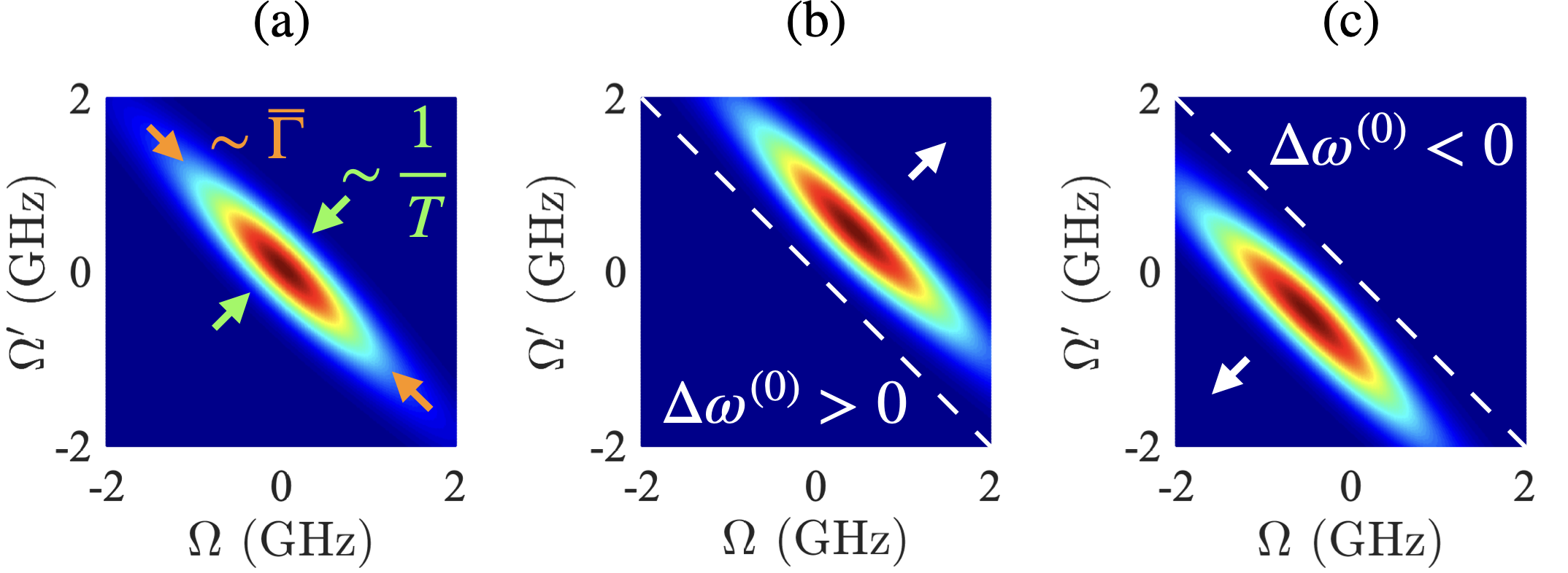
In Appendix A we calculate the biphoton wavefunction describing the photon pair generated in each ring. A typical biphoton wavefunction amplitude $|\phi_{1}(\Omega,\Omega^{\prime})|$ for ring 1 is shown in Fig. 4 (a) for $T=3\,{\rm ns}$, frequency $\omega^{(0)}_{P_{a}}$, and loaded quality factor $Q_{{\rm load},1}=Q_{\rm int}/2$ (i.e., critical coupling). In Fig. 4 (a) the green and red arrows indicate that the width of $|\phi_{1}(\Omega,\Omega^{\prime})|$ in the diagonal direction is inversely proportional to $T$, and the width in the anti-diagonal direction is proportional to the resonance linewidth $\overline{\Gamma}=\omega^{(0)}_{P_{a}}/(2Q_{{\rm load},1})$. For example, by overcoupling the ring to the waveguide (i.e., by increasing $\overline{\Gamma}$) the biphoton wavefunction is stretched along the anti-diagonal, and by decreasing $T$ it is stretched along the diagonal. Thus, by modifying the ring coupling and the pump pulse duration one can adjust each biphoton wavefunction and maximize the overlap integrals $O_{nn^{\prime}}$ in Eq. (39).

The frequency mismatch between the resonances of ring 1 is defined as $\Delta\omega^{(0)}_{1}\equiv 2\omega^{(0)}_{P_{a}}-\omega^{(0)}_{S_{a}}-\omega^{(0)}_{I_{a}}$, which can be approximated with $\Delta\omega^{(0)}_{1}=-2GVD_{P_{a}}(m_{P_{a}}-m_{S_{a}})^{2}/R_{1}^{2}$, where $GVD_{P_{a}}=d^{2}\omega(k)/dk^{2}|_{K_{P_{a}}}$ is the GVD evaluated at the central wavenumber $K_{P_{a}}$ for the pump, $R_{1}$ is the radius of ring 1, and $m_{P_{a}}$ and $m_{S_{a}}$ are the mode numbers for the pump and signal. For normal dispersion $GVD_{P_{a}}>0$ the frequency mismatch is negative $\Delta\omega^{(0)}_{1}<0$, while for anomalous dispersion $GVD_{P_{a}}<0$ it is positive $\Delta\omega^{(0)}_{1}>0$. For ring 1 we calculate $\Delta\omega^{(0)}_{1}=0.0166\,{\rm GHz}$, which will cause the biphoton wavefunction to slightly shift towards positive detuning frequency. In Fig. 4 (b) we exaggerate this shift for illustrative purpose. The frequency mismatch for each of the other rings is $\Delta\omega^{(0)}_{2}=0.0267\,{\rm GHz}$, $\Delta\omega^{(0)}_{3}=0.0174\,{\rm GHz}$, and $\Delta\omega^{(0)}_{4}=0.0279\,{\rm GHz}$, respectively. So each biphoton wavefunction is shifted towards positive frequency detuning by a slightly different amount, which can prevent their overlap integrals from equaling 1.

In Fig. 5 (a) we show the purities $\gamma_{\rm bin}$ (blue line) and $\gamma_{\rm pol}$ (orange dashed) for rings 1 and 2 critically coupled, and rings 3 and 4 having equal but variable coupling efficiencies. The coupling efficiency is defined as

where $0\leq\eta_{n}\leq 1$. For critical coupling $\eta_{n}=1/2$. In our calculations we put $\theta_{3}=\theta_{1}+\theta_{2}$, $T=1\,{\rm ns}$ for both pumps, and use peak powers around $1\,{\rm mW}$. In Fig. 5 (a) the purity for either DOF is maximized when $\eta_{3}=\eta_{4}=1/2$, which gives $\gamma_{\rm pol}=99.942\%$ and $\gamma_{\rm bin}=99.998\%$. Here $\gamma_{\rm pol}$ is insensitive to changes in $\eta_{3}=\eta_{4}$, because it depends on the overlaps $O_{12}$ and $O_{34}$ involving rings with equal coupling efficiencies (i.e., $\eta_{1}=\eta_{2}$ and $\eta_{3}=\eta_{4}$). So we can expect $\phi_{1}(\Omega,\Omega^{\prime})\approx\phi_{2}(\Omega,\Omega^{\prime})$ and $\phi_{3}(\Omega,\Omega^{\prime})\approx\phi_{4}(\Omega,\Omega^{\prime})$. But, $\gamma_{\rm bin}$ is sensitive to changes in $\eta_{3}=\eta_{4}$, because it depends on the overlaps $O_{13}$ and $O_{24}$ involving rings with different coupling efficiencies. So we can expect $\phi_{1}(\Omega,\Omega^{\prime})\neq\phi_{3}(\Omega,\Omega^{\prime})$ and $\phi_{2}(\Omega,\Omega^{\prime})\neq\phi_{4}(\Omega,\Omega^{\prime})$. In Fig. 5 (b) we consider a similar setup as above, except now $\eta_{1}=\eta_{3}=1/2$ and we vary $\eta_{2}=\eta_{4}$. Here we can expect $\phi_{1}(\Omega,\Omega^{\prime})\approx\phi_{3}(\Omega,\Omega^{\prime})$ and $\phi_{2}(\Omega,\Omega^{\prime})\approx\phi_{4}(\Omega,\Omega^{\prime})$, causing the purity $\gamma_{\rm bin}$ to be insensitive to changes in $\eta_{2}=\eta_{4}$. As expected, to obtain the highest purity in both DOFs the coupling efficiencies of all rings should be similar.

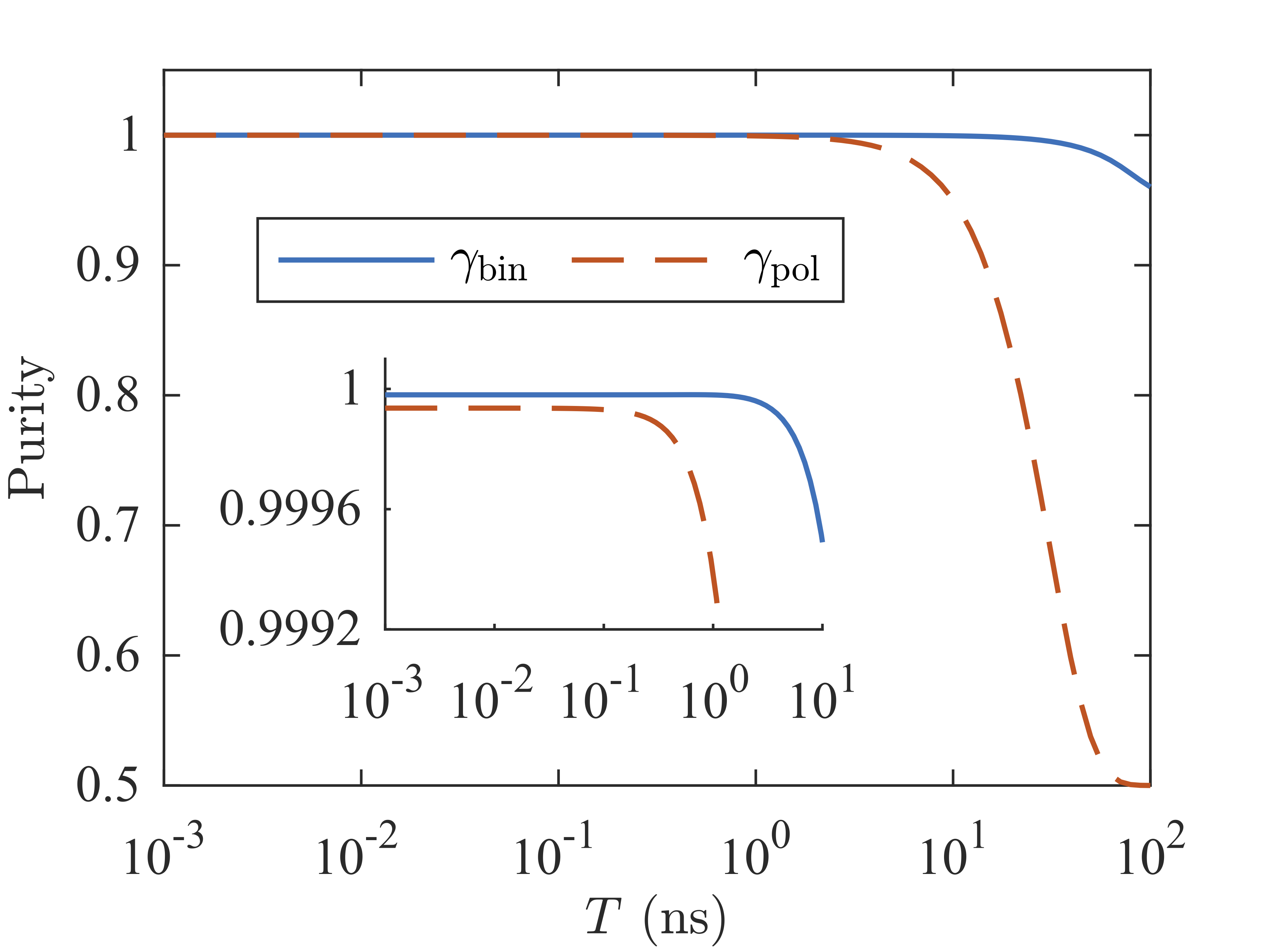
In Fig. 6, we show $\gamma_{\rm pol}$ (orange dashed) and $\gamma_{\rm bin}$ (blue line) for increasing $T$, by considering all rings in critical coupling. For $T$ much shorter than the dwelling time of the photon ($\sim 5\,{\rm ns}$) the width of each biphoton wavefunction ($\sim 1/T$) is generally much larger than the shift of its center caused by $\Delta\omega^{(0)}>0$. The relative shift between two biphoton wavefunctions for a longer $T$, however, can be on the order of their widths. So generally as $T$ increases the overlap integrals (39) approach zero and the purity decreases. For $T=1\,{\rm ns}$ we obtain $\gamma_{\rm pol}=99.939\%$ and $\gamma_{\rm bin}=99.998\%$ (see inset of Fig. 6), and for $T=10\,{\rm ns}$, $\gamma_{\rm pol}=95.021\%$ (a $5\%$ decrease) and $\gamma_{\rm bin}=99.949\%$ (a $0.05\%$ decrease). Increasing $T$ causes $\gamma_{\rm pol}$ to decrease more than $\gamma_{\rm bin}$, because the relative shift in the centers of the biphoton wavefunctions from rings 1 and 2 ($|\Delta\omega^{(0)}_{1}-\Delta\omega^{(0)}_{2}|\approx 0.01\,{\rm GHz}$) is an order of magnitude larger than it is for the biphoton wavefunctions from rings 1 and 3 ($|\Delta\omega^{(0)}_{1}-\Delta\omega^{(0)}_{3}|\approx 0.001\,{\rm GHz}$).

To achieve a high degree of purity in both DOFs in our system the coupling efficiencies of all the rings should be the same and $T$ should not exceed $1\,{\rm ns}$. However, we show in the next section that the generation rate of photon-pairs is large for long pulses. So there is a trade-off between high purity in both DOFs and a large generation rate.

In this section, we analyze the efficiency of the system. Here, we validate this assumption by examining the generation probability for each ring individually, ensuring that the photon pair generation remains within acceptable and practical limits.

To start, we investigate the validity of our assumption that each ring generates at most a pair of photons. First, we consider the state generated by a single ring $n$ and impose the condition that the probability of generating a pair from this ring is small, $|\beta_{n}|^{2}\ll 1$. In Fig. 7 (a), we present $|\beta_{1}|^{2}$ for ring 1 as a function of the peak power incident on the ring, assuming $T=1,{\rm ns}$ and critical coupling, calculated as described in Appendix A. In the results section (Sec. V), where all rings are critically coupled, we set the peak pump power incident on each ring to approximately $1,{\rm mW}$. As shown in Fig. 7 (a), a peak pump power of $1,{\rm mW}$ corresponds to $|\beta_{1}|^{2}=3\times 10^{-4}$, satisfying the condition $|\beta_{1}|^{2}\ll 1$. This result confirms that the assumption of low photon pair generation probability holds for each ring, supporting the overall model used in our analysis.

The rate at which photon pairs are generated by a given ring is the probability of generating a pair divided by the effective pulse duration, $\mathcal{R}_{n}=|\beta_{n}|^{2}/T$. In Fig. 7 (b) we plot the pair-generation rate for ring 1, as a function of $T$, for an incident peak power of $1\,{\rm mW}$. In that figure the rate for $T=1\,{\rm ns}$ is $\mathcal{R}_{1}=3.07\times 10^{5}\,{\rm Hz}$, and given that we have equalized the rate from each ring, the total generation rate for the system is $\mathcal{R}_{\rm tot}\equiv 4\mathcal{R}_{1}=1.23\times 10^{6}\,{\rm Hz}$. Using $T=100\,{\rm ns}$ instead we roughly double the rate ($5.97\times 10^{5}\,{\rm Hz}$) but the purity decreases by approximately $4\%$ for the bin DOF and $50\%$ for the polarization DOF.

We have proposed an integrated circuit design for generating polarization-frequency-bin hyperentangled photon pairs. Both the polarization and frequency-bin degrees of freedom (DOF) of the photon pairs are entangled on-chip through spontaneous four-wave mixing (SFWM) interactions in a series of ring resonators. A programmable sequence of Mach-Zehnder interferometers (MZIs) and add-drop filters is used to control the intensity and phase of the pump pulse incident on each ring. We derived three conditions that must be satisfied to achieve hyperentanglement. First, the pair-generation probability must be equal across all rings. Second, the relative phase between the pumps incident on different rings must maintain a fixed relationship. Third, the biphoton wavefunctions for each ring should be identical, meaning that the continuous frequency DOF characteristics of the photon pairs must be the same for each ring. We demonstrated numerically that these three conditions can be met under realistic system parameters, accounting for variations in the resonance linewidths and dispersion of each ring, and we obtained a generation rate for the hyperentangled state of $10^{6},{\rm Hz}$. Thus, this approach can efficiently generate on-chip polarization-frequency-bin hyperentanglement, and we believe it will be of great interest to those developing quantum information processing with photonic integrated circuits.

The authors would like to acknowledge the Horizon-Europe research and innovation program under Grant Agreement No. 101070168 (HYPERSPACE) for funding this work. J. E. S. and C. V. acknowledge Natural Sciences and Engineering Research Council of Canada for funding.

References

- Alshaari et al. [2020] A. W. Alshaari, W. Pernice, K. Srinivasan, et al., Hybrid integrated quantum photonic circuits, Nat. Photonics 14, 285 (2020).
- Wang et al. [2020] J. Wang, F. Sciarrino, A. Laing, et al., Integrated photonic quantum technologies, Nat. Photonics 14, 273 (2020).
- Wang et al. [2018] J. Wang, S. Paesani, Y. Ding, et al., Multidimensional quantum entanglement with large-scale integrated optics, Science 360, 285 (2018).
- Alshaari et al. [2017] A. W. Alshaari, I. E. Zadeh, A. Fognini, et al., On-chip single photon filtering and multiplexing in hybrid quantum photonic circuits, Nat. Commun 8, 379 (2017).
- Mahmudlu et al. [2023] H. Mahmudlu, R. Johanning, A. van Rees, et al., Fully on-chip photonic turnkey quantum source for entangled qubit/qudit state generation, Nat. Photonics 17, 518 (2023).
- Taballione et al. [2023] C. Taballione, M. C. Anguita, M. de Goede, et al., 20-mode universal quantum photonic processor, Quantum 7, 1071 (2023).
- Qiang et al. [2018] X. Qiang, X. Zhou, J. Wang, et al., Large-scale silicon quantum photonics implementing arbitrary two-qubit processing, Nat. Photonics 12, 534 (2018).
- Pseiner et al. [2021] J. Pseiner, L. Achatz, L. Bulla, et al., Experimental wavelength-multiplexed entanglement-based quantum cryptography, Quantum Sci. Technol. 6, 035013 (2021).
- Yin et al. [2020] J. Yin, Y.-H. Li, S.-K. Liao, et al., Entanglement-based secure quantum cryptography over 1,120 kilometres, Nature 582, 501 (2020).
- Llewellyn et al. [2020] D. Llewellyn, Y. Ding, I. I. Faruque, et al., Chip-to-chip quantum teleportation and multi-photon entanglement in silicon, Nat. Phys. 16, 148 (2020).
- Crespi et al. [2013] A. Crespi, R. Osellame, R. Ramponi, et al., Anderson localization of entangled photons in an integrated quantum walk, Nat. Photonics 7, 322 (2013).
- Sabattoli et al. [2022] F. A. Sabattoli, L. Gianini, A. Simbula, et al., A silicon source of frequency-bin entangled photons, Opt. Lett. 47, 6201 (2022).
- Liscidini and Sipe [2019] M. Liscidini and J. E. Sipe, Scalable and efficient source of entangled frequency bins, Opt. Lett. 44, 2625 (2019).
- Imany et al. [2018] P. Imany, J. A. Jaramillo-Villegas, O. D. Odele, et al., 50-ghz-spaced comb of high-dimensional frequency-bin entangled photons from an on-chip silicon nitride microresonator, Opt. Express 26, 1825 (2018).
- Kues et al. [2017] M. Kues, C. Reimer, P. Roztocki, et al., On-chip generation of high-dimensional entangled quantum states and their coherent control, Nature 546, 622 (2017).
- Reimer et al. [2016] C. Reimer, M. Kues, P. Roztocki, et al., Generation of multiphoton entangled quantum states by means of integrated frequency combs, Science 351, 1176 (2016).
- Kwiat [1997] P. G. Kwiat, Hyper-entangled states, Journal of Modern Optics 44, 2173 (1997).
- Barreiro et al. [2005] J. T. Barreiro, N. K. Langford, N. A. Peters, and P. G. Kwiat, Generation of hyperentangled photon pairs, Phys. Rev. Lett. 95, 260501 (2005).
- Lu et al. [2023] H.-H. Lu, M. Alshowkan, K. V. Myilswamy, A. M. Weiner, J. M. Lukens, and N. A. Peters, Generation and characterization of ultrabroadband polarization–frequency hyperentangled photons, Opt. Lett. 48, 6031 (2023).
- Chiriano et al. [2023] F. Chiriano, J. Ho, C. L. Morrison, J. W. Webb, A. Pickston, F. Graffitti, and A. Fedrizzi, Hyper-entanglement between pulse modes and frequency bins, Opt. Express 31, 35131 (2023).
- Francesconi et al. [2023] S. Francesconi, A. Raymond, R. Duhamel, P. Filloux, A. Lemaître, P. Milman, M. I. Amanti, F. Baboux, and S. Ducci, On-chip generation of hybrid polarization-frequency entangled biphoton states, Photon. Res. 11, 270 (2023).
- Kang et al. [2014] D. Kang, L. G. Helt, S. V. Zhukovsky, J. P. Torres, J. E. Sipe, and A. S. Helmy, Hyperentangled photon sources in semiconductor waveguides, Phys. Rev. A 89, 023833 (2014).
- Ciampini et al. [2016] M. A. Ciampini, A. Orieux, S. Paesani, et al., Path-polarization hyperentangled and cluster states of photons on a chip, Light: Sci. Appl. 5, e16064 (2016).
- Barreiro et al. [2008] J. T. Barreiro, T. Wei, and P. G. Kwiat, Beating the channel capacity limit for linear photonic superdense coding, Nat. Phys. 4, 282 (2008).
- Nemirovsky-Levy et al. [2024] L. Nemirovsky-Levy, U. Pereg, and M. Segev, Increasing quantum communication rates using hyperentangled photonic states, Optica Quantum 2, 165 (2024).
- Kim et al. [2021] J.-H. Kim, Y. Kim, D.-G. Im, et al., Noise-resistant quantum communications using hyperentanglement, Optica 8, 1524 (2021).
- Ecker et al. [2019] S. Ecker, F. Bouchard, L. Bulla, et al., Overcoming noise in entanglement distribution, Phys. Rev. X 9, 041042 (2019).
- Hu et al. [2021] X.-M. Hu, C. Zhang, Y. Guo, et al., Pathways for entanglement-based quantum communication in the face of high noise, Phys. Rev. Lett. 127, 110505 (2021).
- Zhong et al. [2015] T. Zhong, H. Zhou, R. D. Horansky, et al., Photon-efficient quantum key distribution using time–energy entanglement with high-dimensional encoding, New J. Phys. 17, 022002 (2015).
- Sheridan and Scarani [2010] L. Sheridan and V. Scarani, Security proof for quantum key distribution using qudit systems, Phys. Rev. A 82, 030301 (2010).
- Islam et al. [2017] N. T. Islam, C. C. W. Lim, C. Cahall, J. Kim, and D. J. Gauthier, Provably secure and high-rate quantum key distribution with time-bin qudits, Science Advances 3, e1701491 (2017).
- Fiorentino and Wong [2004] M. Fiorentino and F. N. C. Wong, Deterministic controlled-not gate for single-photon two-qubit quantum logic, Phys. Rev. Lett. 93, 070502 (2004).
- Imany et al. [2019] P. Imany, J. A. Jaramillo-Villegas, M. S. Alshaykh, J. M. Lukens, O. D. Odele, A. J. Moore, D. E. Leaird, M. Qi, and A. M. Weiner, High-dimensional optical quantum logic in large operational spaces, npj Quantum Information 5, 59 (2019).
- Castro et al. [2022] J. E. Castro, T. J. Steiner, L. Thiel, A. Dinkelacker, C. McDonald, P. Pintus, L. Chang, J. E. Bowers, and G. Moody, Expanding the quantum photonic toolbox in AlGaAsOI, APL Photonics 7, 096103 (2022).
- Clementi et al. [2023] M. Clementi, F. A. Sabattoli, M. Borghi, L. Gianini, N. Tagliavacche, H. E. Dirani, L. Youssef, N. Bergamasco, C. Petit-Etienne, E. Pargon, J. E. Sipe, M. Liscidini, C. Sciancalepore, M. Galli, and D. Bajoni, Programmable frequency-bin quantum states in a nano-engineered silicon device, Nat. Commun 14, 120 (2023).
- Onodera et al. [2016] T. Onodera, M. Liscidini, J. E. Sipe, and L. G. Helt, Parametric fluorescence in a sequence of resonators: An analogy with dicke superradiance, Phys. Rev. A 93, 043837 (2016).
- Banic et al. [2022] M. Banic, L. Zatti, M. Liscidini, and J. E. Sipe, Two strategies for modeling nonlinear optics in lossy integrated photonic structures, Phys. Rev. A 106, 043707 (2022).
- Schlichtholz et al. [2022] K. Schlichtholz, B. Woloncewicz, and M. Żukowski, Simplified quantum optical stokes observables and bell’s theorem, Scientific Reports 12, 10101 (2022).
Appendix A Appendix A: The Biphoton Wavefunction
For the specific case of photon pairs generated by ring resonators, the biphoton wavefunction in a given ring assuming that the group velocities at the pump, signal, and idler frequencies are approximately equal can be written as [37]