Production of and in ultra-relativistic heavy-ion collisions
Abstract
Even though lots of -hypernuclei have been found and measured, multi-strangeness hypernuclei consisting of are not yet discovered. The studies of multi-strangeness hypernuclei help us further understand the interaction between hyperons and nucleons. Recently the and interactions as well as binding energies were calculated by the HAL-QCD’s lattice Quantum Chromo-Dynamics (LQCD) simulations and production rates of -dibaryon in Au + Au collisions at RHIC and Pb + Pb collisions at LHC energies were estimated by a coalescence model. The present work discusses the production of more exotic triple-baryons including , namely and as well as their decay channels. A variation method is used in calculations of bound states and binding energy of and with the potentials from the HAL-QCD’s results. The productions of and are predicted by using a blast-wave model plus coalescence model in ultra-relativistic heavy-ion collisions at GeV and TeV. Furthermore, plots for baryon number dependent yields of different baryons ( and ), their dibaryons and hypernuclei are made and the production rate of a more exotic tetra-baryon () is extrapolated.
I Introduction
Hypernucleus consisting of hyperons and nucleons is described by not only mass and charge but also hypercharge. Danysz and Pniewski first discovered the from cosmic rays in 1952 Danysz and Pniewski (1953). Since then more attention has been paid to hypernuleus research and many -hypernuclei were discovered in cosmic rays as well as by accelerator beams Davis (2005); Gal et al. (2021). Recently the observation of - was also reported by the J-PARC laboratory Hayakawa et al. (2021). Nowadays, relativistic heavy-ion collisions can produce a large number of strange hyperons Abelev et al. (2010); Chen et al. (2018); Zhang et al. (2021a, 2018), which provides a venue to discover the hypernucleus even anti-hypernucleus. The research on hypernuclei is becoming an important direction in heavy-ion collision experiments Buyukcizmeci et al. (2020). On the other hand, multi-quark exotic hadrons or hadronic molecules are also in current focus in particle and heavy-ion physics Brambilla et al. (2020); Esposito et al. (2017); Qin and Roberts (2020); Chen et al. (2020); Wu et al. (2021); Zhang et al. (2021b); Cho et al. (2017). The HAL-QCD Collaboration reported the most strangeness dibaryon candidates, and Iritani et al. (2019); Gongyo et al. (2018) by the Lattice Quantum Chromo-Dynamics (LQCD) simulations. Based on their results, our previous work calculated the production of and dibaryons and gave the yields of -dibaryon by the blast-wave model or A Multiphase Transport (AMPT) model coupling with a coalescence model in relativistic heavy-ion collisions at GeV and TeV Zhang and Ma (2020).
The attractive nature of the interaction leads to the possible existence of an dibaryon with strangeness = , spin = 2, and isospin = 1/2, which was first proposed in Ref. Goldman et al. (1987). Later on the HAL-QCD Collaboration calculated the - and - interaction by the LQCD simulations near the physical point and the LQCD potentials are fitted by Gaussians and (Yukawa)2. The results lead to the binding energy MeV, MeV and MeV Iritani et al. (2019); Gongyo et al. (2018). The STAR Collaboration made a first measurement of momentum correlation functions of for Au + Au collisions at GeV Adam et al. (2019) which indicates that the scattering length is positive for the proton- interaction and favors the proton- bound state hypothesis by comparing with the predictions based on the proton- interaction extracted from (2 + 1)-flavor LQCD simulations Morita et al. (2016). Later on the ALICE collaboration measured the momentum correlation function of in pp collision at TeV Acharya et al. (2020) which supports the HAL-QCD result Iritani et al. (2019). The potentials given by the HAL-QCD Iritani et al. (2019) are also used to calculate the binding energy of -hypernuclei with = 3. Garcilazo and Valcarce Garcilazo and Valcarce (2019) calculated the bound states of three-body -hypernuclei, namely and , by solving the Faddeev equations Faddeev (1961) with the HAL-QCD potentials and obtained their binding energies ranging from 2 MeV to 20 MeV.
In this work the productions of and are calculated by a coalescence model in which the nucleon and hyperon phase space distributions are given by a blast-wave model Retière and Lisa (2004); Sun and Chen (2017); Zhang et al. (2014); Zhang and Ma (2020). The potentials from the LQCD are taken into account to obtain the relative wave functions and binding energies of and by solving Schrödinger equation via a variation method. The estimation of the yields of and will shed light on searching for -hypernuclei in experiment, such as at LHC-ALICE.
The calculation of production is introduced in Section II, which includes the brief introductions of the blast-wave model and the coalescence model Retière and Lisa (2004); Sun and Chen (2017); Zhang et al. (2014); Zhang and Ma (2020), simplification of Wigner function as well as the variation calculation method of three-body bound state. It is compared with the results from the Faddeev equations used by Garcilazo and Valcarce Garcilazo and Valcarce (2019). In Section III, productions of and are reported for Au + Au collisions at GeV and Pb + Pb collisions at TeV. The decay channels of and are also discussed in this section.
II Method
II.1 Blast-wave model and coalescence model
Cluster formation in heavy-ion collision can be realized by the coalescence model Yan et al. (2006); Schaffner-Bielich et al. (2000); Chen et al. (2003); Zhang et al. (2010); Sun and Chen (2017) or other methods like kinetic approaches Sun et al. (2021a); Staudenmaier et al. (2021); He et al. (2020). In this work, a coalescence model constructed by the particle emission distribution and the Wigner density distribution is used to calculate few-body system production in heavy-ion collisions. The multiplicity of three-constituent-cluster is given by,
| (1) |
where is the Wigner density function which describes the coalescence probability, and is the coalescence statistical factor Polleri et al. (1999); Zhao et al. (2018); Zhu et al. (2015); Sun et al. (2019, 2021b), is the total spin for the three-body system and is the spin for each constituent particle. Table 1 lists the used in this paper for each -hypernucleus ( = 3) and triton.
| Nuclei | ||||||
|---|---|---|---|---|---|---|
| 1/4 | 3/8 | 1/4 | 1/4 | 1/16 | 1/16 |
In this work the particle emission distribution, , is given by the blast-wave model Retière and Lisa (2004); Sun and Chen (2017); Zhang et al. (2014); Zhang and Ma (2020) which can describe the particle phase-space distribution in heavy-ion collisions. It assumes that in the rest frame the distribution of momenta is described by either a Bose or Fermi distribution of single particle and then the distribution is boosted into the center-of-mass frame of the total number of particles to describe the probability of finding a particle Cooper and Frye (1974). In heavy-ion collisions, the freeze-out time is considered following a Gaussian distribution Retière and Lisa (2004); Sun and Chen (2017); Zhang et al. (2014); Zhang and Ma (2020); Waqas et al. (2020). The blast-wave model is formalized as,
| (2) | ||||
where and are the transverse mass and the rapidity of a single particle, and are the radius and azimuthal angle of coordinate space, and are proper time and space pseudorapidity. is the Gaussian distribution of freeze-out proper time, where and are the mean value and dispersion of this distribution. is the Fermi or Bose distribution of a single particle boosted into the center-of-mass frame, where is the spin of the particle, is the four-velocity of a fluid element in the fireball of the particle source and is the freeze-out temperature. The Lorentz invariant can be expressed as,
| (3) | ||||
where is the azimuthal angle in momentum space and is the transverse rapidity of fireball with a transverse radius , defined as . If the parameters (, , , and ) are fixed, the transverse momentum distribution is given as Zhang and Ma (2020):
| (4) |
II.2 Solving three-body bound state
In order to obtain the Wigner function, bound state wave functions of and need to be calculated. The non-relativistic Schrödinger equations of and ’s bound state can be written as,
| (5) |
| (6) |
where is total wave function of three-body system, and are the wave function and coordinate of -th particle, respectively, is relative coordinate between -th and -th particle defined as . The potentials between - and - are the fit results from the HAL-QCD simulation Iritani et al. (2019); Gongyo et al. (2018), and the - potential is taken as the Malfliet-Tjon potential Malfliet and Tjon (1969):
| (7) | ||||
where is taken as MeV (near the physical mass MeV). The parameters are listed in Table 2.
| (MeV) | (MeV) | () | () | ||
| -636.36 | 1460.47 | 1.55 | 3.11 | ||
| -521.74 | 1460.47 | 1.55 | 3.11 | ||
| (MeV) | () | (MeV) | () | ||
| -313.0 (5.3) | 81.7 (5.4) | -252.0 (27.) | 0.85 (10) | ||
| (MeV) | (MeV) | (MeV) | |||
| 914.0 (52) | 305.0 (44) | -112.0 (13) | |||
| 0.143 (5) | 0.305 (29) | 0.949 (58) |
There are many methods to solve this kind of three-body equations, such as the Faddeev equation Faddeev (1961); Thompson et al. (2004); Kovalchuk (2014) and the variation method. One kind of the variation methods is mainly based on the hyperspherical-harmonics (HH) method Kievsky et al. (1993, 1994); Kievsky (1997); Kievsky et al. (1997), in which the coordinates are transformed into center-of-mass frame by using the Jacobi transform,
| (8) |
where is the Jacobi matrix, it reads
| (9) |
where is the mass of th particle, is the total mass, is the total mass of particles 2 and 3, is the reduced mass which normalizes the Jacobi matrix. For simplicity, the indexes of particles are chosen as symmetric as possible. In this article, the particles 2 and 3 prefer to be identical and particle 1 is different for a three-body nucleus. Sequentially the three-body Schrödinger equation separates into the center of mass motion (no effect on binding energy and relative wave function) and the relative motion Chattopadhyay et al. (1996); Khan (2012),
| (10) |
where is defined in a six-dimensional hypersphere coordinate, is the hyperradius, is the hyperpolar angle which ranges from 0 to Chattopadhyay et al. (1996); Khan (2012); He et al. (2015), are the azimuth angles of , and the volume element is . The momentum and angular momentum operators are defined as Kievsky et al. (1993, 1994); Chattopadhyay et al. (1996); Khan (2012); He et al. (2015),
| (11) |
where
| (12) |
The eigen function of is a hyperspherical harmonic function Kievsky et al. (1993, 1994); Kievsky (1997); Kievsky et al. (1997):
| (13) |
and
| (14) |
where is the total hyperangular momentum number, is a nonnegative integer, and is the orbital angular momentum number of direction, represents the -spin-isospin state defined as , is a normalization factor Kovalchuk (2014),
| (15) |
and is the Jacobi polynomial and is the Spherical Harmonic function. The orthogonal basis radial function can be chosen as
| (16) |
in which is a variation parameter, is the radial basis index, is the associated Laguerre polynomial. Then the orthogonal basis function can be constructed as,
| (17) |
Then the relative motion Hamiltonian can be expanded into matrix form . The following assumptions are taken to reduce the dimensions of the matrix: 1) assume that the nucleus is spherical by setting the total = 0, corresponding to the ground state; 2) the is fixed as the same as Garcilazo and Valcarce used Garcilazo and Valcarce (2019); 3) if particle 2 and 3 are identical, the parity between them must be odd Kievsky et al. (1993); 4) , is enough for required precision Kievsky (1997), and the number ranges from 2 to 11 and up to 45. The matrix elements have been calculated numerically by a Laguerre-Gauss quadrature for the integrals in the hyperradius and a Legendre-Gauss quadrature for the hyperangle Abramowitz and Stegun .
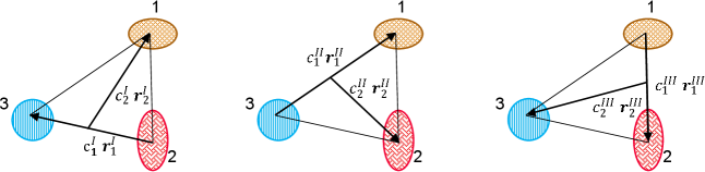
But the elements of Hamiltonian matrix need six dimensional integral and the complex expressions of and for the hypersphere coordinate are based on the transforms of (8) and (9), where . In order to simplify the calculation, Raynal and Revai Raynal and Revai (1970) put forward the RR coefficient which is similar to Clebsch-Gordan coefficient. For example as shown in Fig. 1, it is convenient to calculate when the hypersphere is based on and in Coordinate I but hard to calculate and for the complex expressions of and . By using RR coefficient, the hyperspherical harmonic function , defined in the coordinate I, can be expanded by in coordinate II (III),
| (18) |
where is the RR coefficient which requires that and are same in transformation, and are Clebsch-Gordan coefficients, represents the coordinate II or III, and represent the particle 2 (3) and the pair of particle 3 (1) and 1 (2) when . It is clear that the definition of is same in all coordinates, so the index does not need to change in the transform (18). After the transformation, only relates to the and , which means the six dimensional integral is simplified into a double integral and a sum of .
After the calculation of Hamiltonian matrix, it is natural to calculate the minimum eigenvalue of the matrix as the binding energy of the three-body system and the corresponding eigenvector is the list of coefficients for the basis functions. And the binding energy requires , which means that the binding energy is also the minimum point of variation parameter .
Garcilazo and Valcarce Garcilazo and Valcarce (2016) solved three-body amplitudes by the Faddeev equations Faddeev (1961) with considering the spin and isospin freedom. They assumed that three particles were in -wave by which the spin-isospin state was constructed and two-body amplitudes with the Legendre polynomials were expanded to solve the Faddeev equations.
Table 3 shows the calculated binding energy of , and and the comparison with other theoretical results as well as experimental results. The potential between and used in binding energy calculation is YNG-ND interactions Yamamoto et al. (1994); Hiyama et al. (1997) with Hiyama et al. (2002). It can be seen that this calculation of is consistent with the results from Garcilazo and Valcarce’s results Garcilazo and Valcarce (2019). The error of binding energy is estimated from the fitting errors of the potential. The results of and are close to experimental results Davis (1986); Adam et al. (2020) and theoretical calculations as well Egorov and Postnikov (2021). Like consisting of spin and , one is the ground state (spin ) and one is thought as a virtual state (spin ) near the threshold Schäfer et al. (2022), can also be mix of spin , and . According to the HAL QCD’s calculation Gongyo et al. (2018), the interaction is too weak to form a bound with spin 1. So the ratio of lower spin in is small. In this paper is considered as spin .
| Nuclei | This work | Reference | Experiment Result |
| 8.69 | 8.4 Malfliet and Tjon (1969) | 8.481 (Exp.) | |
| 2.68 | 2.37 Egorov and Postnikov (2021) | (Emulsion) Davis (1986) | |
| (STAR) Adam et al. (2020) | |||
| (ALICE) Acharya et al. (2019) | |||
| 21.3 Garcilazo and Valcarce (2019) | / |
There is another method for few-body system interaction by which the system is not deeply bound, called as the folding model Watanabe (1958); Etminan and Firoozabadi (2019). The folding model assumes that nucleus is bound as a molecular state like dibaryon-baryon state. For the interaction, it is not as strong as , the folding model can be applied in , , and , which softens the interaction. The model uses the free dibaryon wave function to average the potential between dibaryon and baryon,
| (19) | ||||
where is the dibaryon wave function which is consisted of particle 2 and 3, is average potential and the is relative coordinate between the dibaryon and baryon. This method also simplifies the three-body bound state into two two-body bound states (dibaryon and dibaryon-baryon). The total wave function is and total binding energy is , where is the molecular state wave function calculated with the average potential and is the binding energy of molecular state. The binding energies of , , and are calculated by the folding model and their errors are estimated from the fitting error of and potential. The results are listed in Table 4. It can be found that different combinations of dibaryon in three-body systems result in different binding energies which are corresponding to different decay channels and will be discussed later.
| Nuclei | dibaryon-baryon | this work | reference Garcilazo and Valcarce (2019) |
| 2.35 | |||
| 3.04 | |||
| 5.1 | |||
| 6.5 | |||
II.3 Wigner function
The Wigner function introduced in Eq. (1) is written as Chen et al. (2003); Zhang et al. (2010); Sun and Chen (2017),
| (20) | ||||
where , are the relative coordinate and momentum, and is the relative wave function. For the three-body system it is expressed in six dimensions, the Wigner function will be 12 dimensions, which is impossible to draw a picture and hardly calculated. After performing the calculation of eigenvector of Hamiltonian matrix, the major contribution of total wave function comes from a few bases which contribute more than to total amplitude for the parameters of them are large (larger than 0.08). With considering the fitting errors of potential, the total relative errors of such simplified wave functions are about , So this kind of simplification retains most information of origin wave function. If the selected bases are only radial related, the total wave function can be simplified as the sum of these bases with weights of their parameters. And then the simplified wave function is only radial related. The Wigner function can be simplified as,
| (21) | ||||
A Laguerre-Gauss quadrature is applied for the integrals of hyperradius and is integrated by a Legendre-Gauss quadrature Abramowitz and Stegun . The coordinate is defined in a six-dimensional spherical coordinate as , which can be transformed into the six-dimensional Cartesian coordinate:
| (22) | ||||
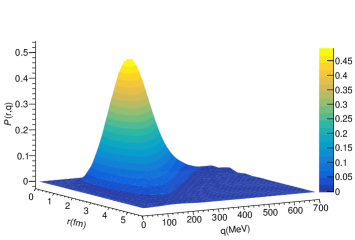
and (), , the volume element is . The in Eq. (21) is set at , the is set at . By integrating out the angle, the probability to find the ground bound state can be obtained at six-dimensional hyperspherical radius and at six-dimensional hyperspherical momentum He et al. (2015),
| (23) |
which is shown in Fig. 2. The Wigner probability is similar to a Gaussian distribution with tails in both coordinate and momentum space. The most probable position in the coordinate-momentum phase space is located at . And the normalization of the probability,
| (24) |
If the wave function relates to not only but also , in other word, the wave function relates to both and which are defined in Fig. 1. Wigner transformation is more complex. can be simplified into . is a 3-dimension radial orthogonal basis which is the same as (16) but the last term is with the same variation parameter for different . Here ranges from 2 to 26 with . By this way, Wigner transformation can be rewritten as:
| (25) | ||||
A complex Wigner transformation is simplified by a series of three-dimension Wigner transform.
For the folding model, , where is the Wigner density function for dibaryon and is the Wigner density function for the pair of dibaryon and third baryon. Both of these two Wigner density functions can be calculated as did in our previous work Zhang and Ma (2020) for two-body systems.
The main errors of Wigner function are from the errors of wave functions. From the relationship between Wigner function and the wave function, the errors of Wigner function are estimated to be about .
III Result and discussion
| T (MeV) | (fm) | (fm) | (fm) | ||
| 200 GeV | 111.6 | 0.98 (0.9) | 15.6 | 10.55 | 3.5 |
| 2.76 TeV | 122 | 1.2 (1.07) | 19.7 | 15.5 | 1 |
In blast-wave model, the parameters (, , , and ) are fitted with experimental transverse momentum spectra of proton and by Eq. (4) and adjusted with the results of triton for different collisions, as shown in Fig. 3. Table 5 listed the parameters used in this work.
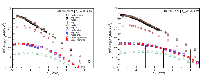
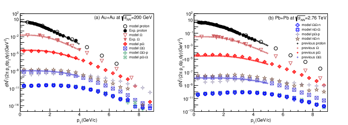
The transverse momentum spectra of is calculated by using the blast-wave model coupled with coalescence model (BLWC) as Eq. (1) and shown in Fig. 3 (a) for Au+Au collisions at GeV and Fig. 3 (b) for Pb + Pb collisions at TeV. The results of with the relative wave function from the folding model are shown in Fig. 4. The spectra of and from our previous work Zhang and Ma (2020) as well as this work are also presented in Fig. 4. The spectra of is not shown here because it is almost as same as .
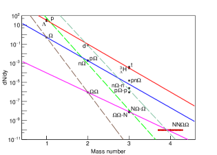
To further investigate the productions of -dibaryons and hypernuclei, the integrated yields at midrapidity are given in Table 6 and 7. The predicted results show Zhang and Ma (2020), , and . The uncertainties of the integrated yields are directly from the Wigner functions, whose relative errors are about . So the relative errors of yields are considered as . Though the uncertainties from the blast-wave parameters are also important, which have been discussed by other model work Zhang et al. (2014), it will not be discussed in this paper. And while, the corresponding values in Pb + Pb collisions at 2.76 TeV are larger than those in Au + Au collisions at 200 GeV. With the growing of constituents number such as and , the production rates appear to follow the exponential function , here is the so-called reduction factor Shah et al. (2016); Xue et al. (2012); Agakishiev et al. (2011), as shown in Fig. 5 for Pb + Pb collisions at 2.76 TeV. This -dependent trend is similar to that for light nuclei of in Fig. 5. However, it can be seen that - (-) slightly deviate from the trend in . Keep in mind that the treatment of interaction is slightly different between and dibaryon-baryon via the folding method, which results in the slight deviation. In general, we have two classes for these production chains. One is for , and (solid lines), they are almost parallel with the increase of constituent number. Another is for , and chains (dash lines), they are almost parallel with the increase of number. Obviously much larger reduction factor for the second class than the first class, indicating that much less yield for adding one more than one more nucleon. The different reduction factor results from the different interactions between and as well as the difference of productions of and . Inspired by this, the production of hypernuclei ( for nucleons and for one kind of hyperons) can be estimated by the intersection of and chains ( is smaller than ). Even if there is one point on the chain of , the reduction factor of this chain is similar to the chain of or other chains whose is known in the same class with . From figure 5, the prediction of the production is about . It implies that the production of hypernuclei is sensitive to the interaction among the constituents in the coalescence framework and then the systematic measurement of hypernuclei can shed light on the production mechanism and the baryon interaction.
| 200 GeV | ||||
|---|---|---|---|---|
| 2.76 TeV |
| 200 GeV | ||||
|---|---|---|---|---|
| 2.76 TeV | ||||
| 200 GeV | ||||
| 2.76 TeV |
can weak decay through an decay, which decays into -hypernuclei ( = 3) or -hypernuclei ( = 3), note that -hypernuclei ( = 3) can not be formed according to the HAL-QCD’s results but might be formed under the ESC08c potential Hiyama et al. (2020). can also strong decay into or which is based on the interaction and reported by the HAL-QCD Sekihara et al. (2018). As for , it can decay into or and mesons from the weak decay of . It can also decay into or by strong interaction. All here mentioned three-baryon group, such as and , may not be bounded.
From Fig. 4, it is hard to figure out the difference between - and -. Although the spectra of - and - are almost the same, the strong decay channels are different in the folding model. For -, it would decay into a or through the or channel and an , while the - can hardly decay into or , since the and are not bound directly in this folding model.
IV Summary
The three-body bound state problem can be solved through a variation method coupled with an eigenvalue problem. For weakly-bounded triple-particle system, the folding model is applied. The - and - potentials used in this work are fitted from the lattice QCD’s simulation near the physical point, which was reported by HAL-QCD collaboration. In coalescence model, the phase-space information of nucleons and are generated by the blast-wave model and the particles are coalesced into and by using the Wigner density function from the simplified three-body wave function. The production of is about and is about . There are also -dependent trends similar with that for . The production rates follow the exponential function . With adding different baryon, the reduction factor is different. Due to different factor , two classes of hypernuclei chains will intersect at certain points where the production rate of new hypernucleus could be estimated. And the decay modes of and are briefly discussed in order to search for such exotic triple-baryons (hypernuclei) in future experiments, which could provide a method to understand the and interactions for multi-strangeness hadrons. The systematic measurements of hypernuclei can definitely shed light on the production mechanism and baryon interactions.
Acknowledgements.
This work was supported in part by the National Natural Science Foundation of China under contract Nos. 11875066, 11890710, 11890714, 11925502, 11961141003, and 12147101, National Key R&D Program of China under Grant No. 2018YFE0104600 and 2016YFE0100900, the Strategic Priority Research Program of CAS under Grant No. XDB34000000, and Guangdong Major Project of Basic and Applied Basic Research No. 2020B0301030008.References
- Danysz and Pniewski (1953) M. Danysz and J. Pniewski, London, Edinburgh, Dublin Philos. Mag. J. Sci. 44, 348 (1953).
- Davis (2005) D. H. Davis, Nucl. Phys. A 754, 3 (2005).
- Gal et al. (2021) A. Gal, E. V. Hungerford, and D. J. Millener, Rev. Mod. Phys. 88, 035004 (2021).
- Hayakawa et al. (2021) S. H. Hayakawa et al. (J-PARC E07 Collaboration), Phys. Rev. Lett. 126, 062501 (2021).
- Abelev et al. (2010) B. I. Abelev et al. (STAR Collaboration), Science 328, 58 (2010).
- Chen et al. (2018) J. Chen, D. Keane, Y.-G. Ma, A. Tang, and Z. Xu, Phys. Rep. 760, 1 (2018).
- Zhang et al. (2021a) D.-C. Zhang, H.-G. Cheng, and Z.-Q. Feng, Chin. Phys. Lett. 38, 092501 (2021a).
- Zhang et al. (2018) S.-H. Zhang, L. Zhou, Y.-F. Zhang, M.-W. Zhang, C. Li, M. Shao, Y.-J. Sun, and Z.-B. Tang, Nucl. Sci. Tech. 29, 136 (2018).
- Buyukcizmeci et al. (2020) N. Buyukcizmeci, A. S. Botvina, R. Ogul, and M. Bleicher, Eur. Phys. J. A 56, 210 (2020).
- Brambilla et al. (2020) N. Brambilla, S. Eidelman, C. Hanhart, et al., Phys. Rep. 873, 1 (2020).
- Esposito et al. (2017) A. Esposito, A. Pilloni, and A. D. Polosa, Phys. Rep. 668, 1 (2017).
- Qin and Roberts (2020) S.-X. Qin and C. D. Roberts, Chin. Phys. Lett. 37, 121201 (2020).
- Chen et al. (2020) H.-X. Chen, W. Chen, R.-R. Dong, and N. Su, Chin. Phys. Lett. 37, 101201 (2020).
- Wu et al. (2021) Q. Wu, D.-Y. Chen, and R. Ji, Chin. Phys. Lett. 38, 071301 (2021).
- Zhang et al. (2021b) H. Zhang, J. Liao, E. Wang, Q. Wang, and H. Xing, Phys. Rev. Lett. 126, 012301 (2021b).
- Cho et al. (2017) S. Cho, T. Hyodo, D. Jido, et al., Prog. Part. Nucl. Phys. 95, 279 (2017).
- Iritani et al. (2019) T. Iritani, S. Aoki, T. Doi, F. Etminan, S. Gongyo, T. Hatsuda, Y. Ikeda, T. Inoue, N. Ishii, T. Miyamoto, and K. Sasaki, Phys. Lett. B 792, 284 (2019).
- Gongyo et al. (2018) S. Gongyo, K. Sasaki, S. Aoki, T. Doi, T. Hatsuda, Y. Ikeda, T. Inoue, T. Iritani, N. Ishii, T. Miyamoto, and H. Nemura, Phys. Rev. Lett. 120, 212001 (2018).
- Zhang and Ma (2020) S. Zhang and Y.-G. Ma, Phys. Lett. B 811, 135867 (2020).
- Goldman et al. (1987) T. Goldman, K. Maltman, G. J. Stephenson, K. E. Schmidt, and F. Wang, Phys. Rev. Lett. 59, 627 (1987).
- Adam et al. (2019) J. Adam et al. (STAR Collaboration), Phys. Lett. B 790, 490 (2019).
- Morita et al. (2016) K. Morita, A. Ohnishi, F. Etminan, and T. Hatsuda, Phys. Rev. C 94, 031901 (2016).
- Acharya et al. (2020) S. Acharya et al. (ALICE Collaboration), Nature 588, 232 (2020).
- Garcilazo and Valcarce (2019) H. Garcilazo and A. Valcarce, Phys. Rev. C 99, 014001 (2019).
- Faddeev (1961) L. D. Faddeev, SOVIET PHYSICS JETP 12, 1014 (1961).
- Retière and Lisa (2004) F. Retière and M. A. Lisa, Phys. Rev. C 70, 044907 (2004).
- Sun and Chen (2017) K. J. Sun and L. W. Chen, Phys. Rev. C 95, 044905 (2017).
- Zhang et al. (2014) S. Zhang, L. X. Han, Y. G. Ma, J. H. Chen, and C. Zhong, Phys. Rev. C 89, 034918 (2014).
- Yan et al. (2006) T. Z. Yan, Y. G. Ma, and X. Z. Cai et al., Phys. Lett. B 638, 50 (2006).
- Schaffner-Bielich et al. (2000) J. Schaffner-Bielich, R. Mattiello, and H. Sorge, Phys. Rev. Lett. 84, 4305 (2000).
- Chen et al. (2003) L.-W. Chen, C. Ko, and B.-A. Li, Nucl. Phys. A 729, 809 (2003).
- Zhang et al. (2010) S. Zhang, J. H. Chen, H. Crawford, D. Keane, Y. G. Ma, and Z. B. Xu, Phys. Lett. B 684, 224 (2010).
- Sun et al. (2021a) K.-J. Sun, R. Wang, C. M. Ko, Y.-G. Ma, and C. Shen, arXiv e-prints (2021a), arXiv:2106.12742 .
- Staudenmaier et al. (2021) J. Staudenmaier, D. Oliinychenko, J. M. Torres-Rincon, and H. Elfner, Phys. Rev. C 104, 034908 (2021).
- He et al. (2020) Y.-J. He, C.-C. Guo, J. Su, L. Zhu, and Z.-D. An, Nucl. Sci. Tech. 31, 84 (2020).
- Polleri et al. (1999) A. Polleri, R. Mattiello, I. N. Mishustin, and J. P. Bondorf, Nucl. Phys. A 661, 452 (1999).
- Zhao et al. (2018) W. Zhao, L. Zhu, H. Zheng, C. M. Ko, and H. Song, Phys. Rev. C 98, 054905 (2018).
- Zhu et al. (2015) L. Zhu, C. M. Ko, and X. Yin, Phys. Rev. C 92, 064911 (2015).
- Sun et al. (2019) K.-J. Sun, C. M. Ko, and B. Dönigus, Phys. Lett. B 792, 132 (2019).
- Sun et al. (2021b) K.-J. Sun, C. M. Ko, and Z.-W. Lin, Phys. Rev. C 103, 064909 (2021b).
- Cooper and Frye (1974) F. Cooper and G. Frye, Phys. Rev. D 10, 186 (1974).
- Waqas et al. (2020) M. Waqas, F.-H. Liu, L.-L. Li, and H. M. Alfanda, Nucl. Sci. Tech. 31, 109 (2020).
- Malfliet and Tjon (1969) R. Malfliet and J. Tjon, Nucl. Phys. A 127, 161 (1969).
- Thompson et al. (2004) I. Thompson, F. Nunes, and B. Danilin, Comput. Phys. Commun. 161, 87 (2004).
- Kovalchuk (2014) V. I. Kovalchuk, Int. J. Mod. Phys. E 23, 1450069 (2014).
- Kievsky et al. (1993) A. Kievsky, M. Viviani, and S. Rosati, Nucl. Phys. A 551, 241 (1993).
- Kievsky et al. (1994) A. Kievsky, M. Viviani, and S. Rosati, Nucl. Phys. A 577, 511 (1994).
- Kievsky (1997) A. Kievsky, Nucl. Phys. A 624, 125 (1997).
- Kievsky et al. (1997) A. Kievsky, L. E. Marcucci, S. Rosati, and M. Viviani, Few-Body Syst. 22, 1 (1997).
- Chattopadhyay et al. (1996) R. Chattopadhyay, T. K. Das, and P. K. Mukherjee, Phys. Scr. 54, 601 (1996).
- Khan (2012) M. A. Khan, Eur. Phys. J. D 66, 83 (2012).
- He et al. (2015) H. He, Y. Liu, and P. Zhuang, Phys. Lett. B 746, 59 (2015).
- (53) M. Abramowitz and I. A. Stegun, Handbook of Mathematical Functions, 0009th ed. (Dover Publications).
- Raynal and Revai (1970) J. Raynal and J. Revai, Nuovo Cim. A Ser. 10 68, 612 (1970).
- Garcilazo and Valcarce (2016) H. Garcilazo and A. Valcarce, Phys. Rev. C 93, 034001 (2016).
- Yamamoto et al. (1994) Y. Yamamoto, T. Motoba, H. Himeno, K. Ikeda, and S. Nagata, Prog. Theor. Phys. Suppl. 117, 361 (1994).
- Hiyama et al. (1997) E. Hiyama, M. Kamimura, T. Motoba, T. Yamada, and Y. Yamamoto, Prog. Theor. Phys. 97, 881 (1997).
- Hiyama et al. (2002) E. Hiyama, M. Kamimura, T. Motoba, T. Yamada, and Y. Yamamoto, Phys. Rev. C 66, 024007 (2002).
- Davis (1986) D. H. Davis, Contemp. Phys. 27, 91 (1986).
- Adam et al. (2020) J. Adam et al. (STAR Collaboration), Nat. Phys. 16, 409 (2020).
- Egorov and Postnikov (2021) M. V. Egorov and V. I. Postnikov, Nucl. Phys. A 1009, 122172 (2021).
- Schäfer et al. (2022) M. Schäfer, B. Bazak, N. Barnea, A. Gal, and J. Mareš, Phys. Rev. C 105, 015202 (2022).
- Acharya et al. (2019) S. Acharya et al. (ALICE Collaboration), Phys. Lett. B 797, 134905 (2019).
- Watanabe (1958) S. Watanabe, Nucl. Phys. 8, 484 (1958).
- Etminan and Firoozabadi (2019) F. Etminan and M. M. Firoozabadi, arXiv e-prints , arXiv:1908.11484 (2019).
- Sun and Chen (2015) K.-J. Sun and L.-W. Chen, Phys. Lett. B 751, 272 (2015).
- Adler et al. (2004) S. S. Adler et al. (PHENIX Collaboration), Phys. Rev. C 69, 034909 (2004).
- Abelev et al. (2009) B. I. Abelev et al. (STAR Collaboration), arXiv e-prints , arXiv:0909.0566 (2009).
- Abelev et al. (2013) B. Abelev et al. (ALICE Collaboration), Phys. Rev. C 88, 044910 (2013).
- Adam et al. (2016a) J. Adam et al. (ALICE Collaboration), Phys. Rev. C 93, 24917 (2016a).
- Abelev et al. (2014) B. Abelev et al., Phys. Lett. B 728, 216 (2014).
- Adam et al. (2007) J. Adam et al. (STAR Collaboration), Phys. Rev. Lett. 98, 062301 (2007).
- Zhang (2021) D. Zhang, Nucl. Phys. A 1005, 121825 (2021).
- Adam et al. (2016b) J. Adam et al. (ALICE Collaboration), Phys. Lett. B 754, 360 (2016b).
- Shah et al. (2016) N. Shah, Y. G. Ma, J. H. Chen, and S. Zhang, Phys. Lett. B 754, 6 (2016).
- Xue et al. (2012) L. Xue, Y. G. Ma, J. H. Chen, and S. Zhang, Phys. Rev. C 85, 064912 (2012).
- Agakishiev et al. (2011) H. Agakishiev et al. (STAR Collaboration), Nature 473, 353 (2011).
- Hiyama et al. (2020) E. Hiyama, K. Sasaki, T. Miyamoto, T. Doi, T. Hatsuda, Y. Yamamoto, and T. A. Rijken, Phys. Rev. Lett. 124, 092501 (2020).
- Sekihara et al. (2018) T. Sekihara, Y. Kamiya, and T. Hyodo, Phys. Rev. C 98, 015205 (2018).