Processes $\gamma\gamma\rightarrow\phi_{i}\phi_{j}$ in Inert Higgs Doublet Models and Two Higgs Doublet Models

Khiem Hong Phan [email protected] Dzung Tri Tran Thanh Huy Nguyen Institute of Fundamental and Applied Sciences, Duy Tan University, Ho Chi Minh City

70000

, Vietnam Faculty of Natural Sciences, Duy Tan University, Da Nang City

50000

, Vietnam VNUHCM-University of Science,

227

Nguyen Van Cu, District

5

, Ho Chi Minh City

70000

, Vietnam

Abstract

In this paper, we present the results for one-loop induced processes $\gamma\gamma\rightarrow\phi_{i}\phi_{j}$ with CP-even Higgses $\phi_{i,j}\equiv h,\leavevmode\nobreak\ H$ at high energy photon-photon collision, within the frameworks of Inert Higgs Doublet Models and Two Higgs Doublet Models. Total cross-sections are shown as functions of center-of-mass energies. We find that the cross-sections for the computed processes in all the models under investigations are enhanced at around the threshold of singly charged Higgs pair ( $\sim 2M_{H^{\pm}}$ ). Furthermore, the enhancement factors defined as the ratio of cross-sections of $\gamma\gamma\rightarrow\phi_{i}\phi_{j}$ in the investigated models over the corresponding ones for $\gamma\gamma\rightarrow hh$ in the Standard Model, are examined in the model’s parameter space. In the Inert Higgs Doublet Models, the factors are studied in the parameter space of $(M_{H^{\pm}},\leavevmode\nobreak\ \mu^{2}_{2})$ and $(M_{H^{\pm}},\leavevmode\nobreak\ \lambda_{2})$ . In the Two Higgs Doublet Models, the factors are examined in the planes of $(M_{H^{\pm}},\leavevmode\nobreak\ t_{\beta})$ as well as in the space of charged Higgs mass $M_{H^{\pm}}$ and the soft-breaking $Z_{2}$ parameter $m_{12}^{2}$ . Two scenarios of $c_{\beta-\alpha}>0$ and $c_{\beta-\alpha}<0$ are studied in further detail. The factors give a different behavior from considering these scenarios. As a result, discriminations for the above-mentioned scenarios can be performed at future colliders.

keywords:

Higgs phenomenology, one-loop corrections, analytic methods for quantum field theory, dimensional regularization.

1 Introduction

Measuring for scalar Higgs self-couplings including Standard Model-like Higgs trilinear- and quadratic-couplings as well as the couplings between scalar Higgses in many physics beyond the Standard Models (BSM) plays a key role for determining the scalar potential. We can subsequently answer for the origin of the electroweak symmetry breaking (EWSB). In this scheme, Higgs boson pair productions and multi-scalar Higgs productions should be measured precisely at future colliders. Recently, search for Higgs boson pair productions in the two bottom quarks associated with two photons, four bottom quarks, etc in the final states in proton-proton collisions have been performed at the Large Hadron Colliders (LHC) as in [1, 2, 3, 4, 5, 6, 7, 8, 9, 10, 11, 12]. It is well-known that the measurements for Higgs self-couplings are rather challenging at the LHC. The results from the study of [13, 14] show that the expected accuracy in the measurement of trilinear Higgs self-couplings would be about $20\%-30\%$ at the high luminosity of $3000$ fb^-1. We know that physics the future lepton colliders (LC) will be complementary to the LHC in many aspects, as studied in [15]. Furthermore, the LC can significantly improve the LHC measurements in many cases and more important photon-photon collision is an option of the LC [16, 17] which the scalar Higgs pair productions ( $\phi_{i}\phi_{j}$ ) can be measured via the channels $f\bar{f}\rightarrow f\bar{f}\gamma^{*}\gamma^{*}\rightarrow f\bar{f}\phi_{i}\phi_{j}$ for $f\equiv e,\mu$ . In this aspect, the LC could open a window for probing new physics signals through multi-scalar Higgs productions.

From theoretical calculation side, one-loop corrections to double Higgs productions at the LHC have calculated in Standard Model (SM), the Higgs Extensions of the Standard Models (HESM), as well as other BSM frameworks by many groups. For examples, it is worth to mention typical works as in [18, 19, 20, 21, 22, 23, 24, 25, 26, 27, 28, 29, 30, 31, 32, 33, 34, 35, 36, 37, 38, 39, 40, 41, 42, 43, 44, 45, 46, 47, 48, 49, 50, 51, 52, 53, 54, 55, 56, 57, 58, 59, 60, 61, 62, 63, 64, 65, 66, 67, 68, 69, 70, 71, 72, 73, 74, 75, 76, 77, 78], for further reviews in [79] and the related-references therein. Additionally, one-loop induced for $hh$ productions in the high-energy $\gamma\gamma$ collisions in the SM, the HESM and other BSMs have computed in Refs. [80, 81, 82, 83, 84, 85, 86, 87, 88, 89, 90, 91, 92, 93, 94]. Other computations for one-loop induced for Higgs boson pair productions in the linear lepton colliders including future multi-TeV muon colliders, have performed in Refs. [95, 96, 97, 98] and the additional references therein. Furthermore, double pseudo-scalar Higgs $A^{0}A^{0}$ at a $\gamma\gamma$ collider in the Two Higgs Doublet Model have reported in Ref. [99].

In this paper, we present the results for one-loop induced processes $\gamma\gamma\rightarrow\phi_{i}\phi_{j}$ with CP-even Higgses $\phi_{i,j}\equiv h,\leavevmode\nobreak\ H$ at high-energy $\gamma\gamma$ collision within the Higgs Extensions of the Standard Models (HESM) including the Inert Higgs Doublet Models the Two Higgs Doublet Models. A general analytic formulas for the process amplitudes derived in ’t Hooft-Feynman gauge (HF) are valid for a class of the above-mentioned HESM. Analytic results for the calculated processes are presented via the scalar Passarino-Veltman (PV) functions following the output of the packages LoopTools [100] and Collier [101]. The analytical expressions are tested by several numerical checks , e.g the ultraviolet finiteness, infrared finiteness of the one-loop amplitudes. Furthermore, the amplitudes also obey the ward identity which the indentity is also verified numerically in the works. Additionally, both the packages LoopTools and Collier are used for cross-checking for the final results before generating physical results. In phenomenological results, cross-sections are shown as functions of center-of-mass energies. Furthermore, the enhancement factors defined as the ratio of cross-sections of $\gamma\gamma\rightarrow\phi_{i}\phi_{j}$ in the HESMs over the corresponding ones for $\gamma\gamma\rightarrow hh$ in the Standard Model, are examined in parameter space of the models under consideration.

The paper is structured as follows. We review briefly the HESM in the next section. We then present calculations for $\gamma\gamma\rightarrow\phi_{i}\phi_{j}$ with CP-even Higgses $\phi_{i,j}\equiv h,H$ in the HESM in the section $3$ . The phenomenological studies for the HESM are discussed in section $4$ . In section $5$ , conclusion and outlook for the paper are shown. In appendices $A,\leavevmode\nobreak\ B$ we derive the couplings appear in the calculations.

2 Higgs Extensions of the Standard Model

Two typical Higgs Extensions of the Standard Models are studied in this paper. The first model is to the Inert Higgs Doublet Models which are reviewed in next subsection $2.1$ . We then discuss the Two Higgs Doublet Models in subsection $2.2$ .

2.1 Inert Higgs Doublet Models

In the IHDM, an inert scalar $SU(2)_{L}$ doublet is included into the potential of the SM. The inert scalar particles will respond for dark matter candidates. For reviewing the theory and phenomenological examinations for the IHDM in concrete, we cite to the following papers [104, 105, 106, 107, 108, 109, 110, 111, 112, 113, 114, 115, 116]. The scalar potential of the IHDM read the general expression as follows:

	$\displaystyle\mathcal{V}_{\textrm{IHDM}}(\phi_{1},\phi_{2})$	$\displaystyle=$	$\displaystyle\mu_{1}^{2}\|\phi_{1}\|^{2}+\mu_{2}^{2}\|\phi_{2}\|^{2}+\lambda_{1}\|\phi_{1}\|^{4}+\lambda_{2}\|\phi_{2}\|^{4}+\lambda_{3}\|\phi_{1}\|^{2}\|\phi_{2}\|^{2}+\lambda_{4}\|\phi_{1}^{\dagger}\phi_{2}\|^{2}$		(1)
			$\displaystyle+\frac{\lambda_{5}}{2}\left\{(\phi_{1}^{\dagger}\phi_{2})^{2}+{\rm h.c}\right\}.$		(1)

The potential is conserved with respect to the so-called the global $Z_{2}$ -symmetry, e.g. $\phi_{1}\leftrightarrow+\phi_{1}$ , $\phi_{2}\leftrightarrow-\phi_{2}$ . In this case, the scalar $\phi_{2}$ is odd and $\phi_{1}$ , all particles in the SM are even under the $Z_{2}$ -transformation. As mentioned, the $Z_{2}$ -symmetry is unbroken after the EWSB, the field $\phi_{2}$ has the zero of vacuum expectation values (VEV). Otherwise, the field $\phi_{1}$ develops non-zero VEV ( $v$ ). Two scalar fields are then expanded around VEV for the EWSB as follows:

	$\displaystyle\phi_{1}$	$\displaystyle=$	$\displaystyle\left(\begin{array}[]{c}G^{\pm}\\ \frac{1}{\sqrt{2}}(v+h+iG^{0})\\ \end{array}\right),$		(4)
	$\displaystyle\phi_{2}$	$\displaystyle=$	$\displaystyle\left(\begin{array}[]{c}H^{\pm}\\ \frac{1}{\sqrt{2}}(H+iA^{0})\\ \end{array}\right).$		(7)

Where the VEV is fixed at $v\sim 246$ GeV (as the SM case). The Goldstone bosons $G^{\pm},\;G^{0}$ are giving the masses for $W^{\pm}$ boson and $Z$ boson, respectively. There is no mixing between $h$ and $H$ . The physical spectrum of the IHDM after the EWSB is consisted of three neutral scalar physical states, e.g two CP-even Higgses $h,\leavevmode\nobreak\ H$ and a CP-odd Higgs $A_{0}$ . In further, we have pair of singly charged Higgs bosons $H^{\pm}$ in this model. In the spectrum, neutral scalar Higgs $h$ is identical to the SM-like Higgs boson discovered at the LHC. The masses of scalar bosons are calculated from the pare parameters as follows:

$\displaystyle M_{h}^{2}$	$\displaystyle=$	$\displaystyle-2\mu_{1}^{2}=2\lambda_{1}v^{2},$	(8)
$\displaystyle M_{H}^{2}$	$\displaystyle=$	$\displaystyle\mu_{2}^{2}+\frac{v^{2}}{2}\lambda_{L},$	(9)
$\displaystyle M_{A^{0}}^{2}$	$\displaystyle=$	$\displaystyle\mu_{2}^{2}+\frac{v^{2}}{2}\lambda_{R},$	(10)
$\displaystyle M_{H^{\pm}}^{2}$	$\displaystyle=$	$\displaystyle\mu_{2}^{2}+\frac{v^{2}}{2}\lambda_{3}.$	(11)

Where we have used $\lambda_{L/R}=\lambda_{3}+\lambda_{4}\pm\lambda_{5}$ . As we mentioned in the above paragraphs, the global $Z_{2}$ -symmetry is unbroken after the EWSB, The "inert" Higgs bosons like $H^{\pm}$ , $A^{0}$ and $H$ have odd number under the $Z_{2}$ -transformation. Subsequently, the "inert" Higgs bosons don’t couple to the SM particles. Therefore, the lightest neutral scalar bosons may be considered as dark matter candidates.

As a consequent of the unbroken of the $Z_{2}$ -symmetry, the Yukawa Lagrangian of the IHDM must be the same as that of the SM. In detail, the Yukawa Lagrangian is expressed as follows:

\displaystyle\mathcal{L}^{\textrm{IHDM}}_{\rm Yukawa}=-\sum_{f=u,d,\ell}g_{hff}\cdot h\bar{f}f+\cdots,

(12)

where the Yukawa coupling is given $g_{hff}=m_{f}/v$ for fermion $f$ . All the couplings involving to the computed processes $\gamma\gamma\rightarrow\phi_{i}\phi_{j}$ in the IHDM are listed in Table 1 (for all physical couplings) and Table 2 (for unphysical particles). We emphasize that the processes $\gamma\gamma\rightarrow hH$ are forbidden in the IHDM due to the $Z_{2}$ -symmetry. Therefore, we have only $\phi_{i}\phi_{j}\equiv hh,\leavevmode\nobreak\ HH$ in this case. The detailed expressions for all the concerned-couplings are derived in the appendix $A$ .

Vertices	Notations	Coupling
$hW_{\mu}W_{\nu}$	$g_{hWW}\cdot g_{\mu\nu}$	$i\left(\dfrac{2M_{W}^{2}}{v}\right)\cdot g_{\mu\nu}$
$hZ_{\mu}Z_{\nu}$	$g_{hZZ}\cdot g_{\mu\nu}$	$i\left(\dfrac{M_{Z}^{2}}{v}\right)\cdot g_{\mu\nu}$
$hH^{\pm}{H^{\mp}}$	$g_{hH^{\pm}H^{\mp}}$	$i\dfrac{2(\mu_{2}^{2}-M_{H^{\pm}}^{2})}{v}$
$Z_{\mu}H^{\pm}(p_{1})H^{\mp}(p_{2})$	$g_{ZH^{\pm}H^{\mp}}\cdot(p_{1}-p_{2})_{\mu}$	$i\left(\dfrac{M_{Z}c_{2W}}{v}\right)\cdot(p_{1}-p_{2})_{\mu}$
$A_{\mu}H^{\pm}(p_{1})H^{\mp}(p_{2})$	$g_{AH^{\pm}H^{\mp}}\cdot(p_{1}-p_{2})_{\mu}$	$i\left(\dfrac{M_{Z}s_{2W}}{v}\right)\cdot(p_{1}-p_{2})_{\mu}$
$hhh$	$g_{hhh}$	$-i\left(\dfrac{3M_{h}^{2}}{v}\right)$
$hHH$	$g_{hHH}$	$i\dfrac{2(\mu_{2}^{2}-M_{H}^{2})}{v}$
$H(p_{2})H^{\pm}(p_{1})W^{\mp}_{\mu}$	$g_{HH^{\pm}W}\cdot(p_{1}-p_{2})_{\mu}$	$\pm i\left(\dfrac{M_{W}}{v}\right)\cdot(p_{1}-p_{2})_{\mu}$
$H^{\pm}H^{\mp}A_{\mu}A_{\nu}$	$g_{AAH^{\pm}H^{\mp}}\cdot g_{\mu\nu}$	$i\left(\dfrac{M_{Z}^{2}s_{2W}^{2}}{v^{2}}\right)\cdot g_{\mu\nu}$
$HH^{\pm}W^{\mp}_{\nu}A_{\mu}$	$g_{HH^{\pm}WA}\cdot g_{\mu\nu}$	$i\left(\dfrac{2M_{Z}^{2}c_{W}^{2}s_{W}}{v^{2}}\right)\cdot g_{\mu\nu}$
$hhH^{\pm}H^{\mp}$	$g_{hhH^{\pm}H^{\mp}}$	$i\dfrac{2(\mu_{2}^{2}-M_{H^{\pm}}^{2})}{v^{2}}$
$HHH^{\pm}H^{\mp}$	$g_{HHH^{\pm}H^{\mp}}$	$-2i\lambda_{2}$
$hhW^{\pm}_{\mu}W^{\mp}_{\nu}$	$g_{hhWW}\cdot g_{\mu\nu}$	$i\left(\dfrac{2M_{Z}^{2}c_{W}^{2}}{v^{2}}\right)\cdot g_{\mu\nu}$
$HHW^{\pm}_{\mu}W^{\mp}_{\nu}$	$g_{HHWW}\cdot g_{\mu\nu}$	$i\left(\dfrac{2M_{Z}^{2}c_{W}^{2}}{v^{2}}\right)\cdot g_{\mu\nu}$

Table 1: We list all couplings (physical couplings) contributing to

\gamma\gamma\rightarrow\phi_{i}\phi_{j}

for the IHDM.

Vertices	Notations	Coupling
$A_{\mu}W^{\pm}_{\nu}G^{\mp}$	$g_{AW^{\pm}G^{\mp}}\cdot g_{\mu\nu}$	$i\left(\dfrac{2M_{Z}^{2}c_{W}^{2}s_{W}}{v}\right)\cdot g_{\mu\nu}$
$HH^{\pm}G^{\mp}$	$g_{HH^{\pm}G^{\mp}}$	$i\dfrac{M_{H^{\pm}}^{2}-M_{H}^{2}}{v}$
$hhG^{\pm}G^{\mp}$	$g_{hhG^{\pm}G^{\mp}}$	$-i\left(\dfrac{M_{h}^{2}}{v^{2}}\right)$
$HHG^{\pm}G^{\mp}$	$g_{HHG^{\pm}G^{\mp}}$	$i\dfrac{2(\mu_{2}^{2}-M_{H^{\pm}}^{2})}{v^{2}}$
$A_{\mu}A_{\nu}G^{\pm}G^{\mp}$	$g_{AAG^{\pm}G^{\mp}}\cdot g_{\mu\nu}$	$i\left(\dfrac{M_{Z}^{2}s_{2W}^{2}}{v^{2}}\right)\cdot g_{\mu\nu}$
$A_{\mu}G^{\pm}(p_{1})G^{\mp}(p_{2})$	$g_{AG^{\pm}G^{\mp}}\cdot(p_{1}-p_{2})_{\mu}$	$i\left(\dfrac{M_{Z}s_{2W}}{v}\right)\cdot(p_{1}-p_{2})_{\mu}$

Table 2: We list all vertices (unphysical couplings) in processes

\gamma\gamma\rightarrow\phi_{i}\phi_{j}

in the IHDM.

The parameter space of the IHDM for our analysis is included as follows:

\displaystyle\mathcal{P}_{\rm IHDM}=\{\mu_{2}^{2},\lambda_{2}^{2},M_{h}^{2}\sim 125.\textrm{GeV},M_{H}^{2},M_{A^{0}}^{2},M^{2}_{H^{\pm}}\}.

(13)

We are going to review the current constraints on the physical parameter space in the IHDM given in Eq. 13. The constraints for the physical parameter space can be obtained by including the theoretical conditions and the experimental data. In the perspective of the experimental data, we take into account the Electroweak Precision Tests (EWPT) of the IHDM, dark matter search at the LHC, as well as including the LEP data. The topics have studied in Refs. [104, 105, 106, 107]. Additionally, the implications for loop-induced decays of the SM-like Higgs ( $h$ ) to $V\gamma$ with $V\equiv Z,\gamma$ in the IHDM framework, e.g. decay process $h\rightarrow\gamma\gamma$ have reported in [108, 115, 116], and decay chanels $h\rightarrow Z\gamma$ have examined in [115, 116]. Furthermore, searching signals of the IHDM at future colliders have performed in Refs. [109, 110, 111, 112, 113, 114]. In the theoretical side, the most important theoretical constraints are obtained from the conditions that the models follow the tree-level unitarity, the vacuum stability, the perturbative regime. The theoretical constraints give the limitations on the Higgs self-couplings $\lambda_{i}$ for $i=1,2,\cdots,5$ and $\mu_{2}$ . Taking theoretical and experimental constraints in the above-mentioned papers, one can select the parameter space for the IHDM as follows: we can take $5$ GeV $\leq M_{H}\leq 150$ GeV, $70$ GeV $\leq M_{H^{\pm}},M_{A^{0}}\leq 1000$ GeV, $|\mu_{2}|\leq 500$ GeV, and $0\leq\lambda_{2}\leq 8\pi$ .

2.2 Two Higgs Doublet Models

We next to consider the second kind of the Higgs extension of the SM which is to the Two Higgs Doublet Models (THDM) in this paper. For reviewing the theory and the phenomenological studies for the THDM, we refer the paper Ref. [117] for further information. The model is summarized briefly in this section. An complex Higgs doublet possessing hypercharge $Y=1/2$ is added into the scalar sector of the SM. The scalar potential is read the form of

	$\displaystyle\mathcal{V}_{\textrm{THDM}}(\phi_{1},\phi_{2})$	$\displaystyle=$	$\displaystyle m_{11}^{2}\phi_{1}^{\dagger}\phi_{1}+m_{22}^{2}\phi_{2}^{\dagger}\phi_{2}-\Big{[}m_{12}^{2}\phi_{1}^{\dagger}\phi_{2}+{\rm h.c.}\Big{]}+\frac{\lambda_{1}}{2}(\phi_{1}^{\dagger}\phi_{1})^{2}+\frac{\lambda_{2}}{2}(\phi_{2}^{\dagger}\phi_{2})^{2}$		(14)
			$\displaystyle+\lambda_{3}(\phi_{1}^{\dagger}\phi_{1})(\phi_{2}^{\dagger}\phi_{2})+\lambda_{4}(\phi_{1}^{\dagger}\phi_{2})(\phi_{2}^{\dagger}\phi_{1})+\frac{1}{2}[\lambda_{5}\leavevmode\nobreak\ (\phi_{1}^{\dagger}\phi_{2})^{2}+\leavevmode\nobreak\ {\rm h.c}].$		(14)

In the present work, the CP-conserving case of the THDM is examined. Subsequently, the pare parameters in the above potential are set to be real parameters in this version. Additionally, the potential of the THDM follows the $Z_{2}$ -symmetry, e.g. $\phi_{1}\leftrightarrow\phi_{1}$ and $\phi_{2}\leftrightarrow-\phi_{2}$ , up to the soft breaking terms as $m_{12}^{2}\phi_{1}^{\dagger}\phi_{2}+{\rm h.c.}$ are added into the potential. Where the parameter $m_{12}^{2}$ is the breaking scale for the $Z_{2}$ -symmetry.

Two scalar doublets are exanded around their VEVs for the EWSB as

\displaystyle\phi_{k}

\displaystyle=

\displaystyle\begin{bmatrix}\rho_{k}^{+}\\ (v_{k}+\eta_{k}+i\xi_{k})/\sqrt{2}\end{bmatrix}\quad\textrm{for}\quad k=1,2.

(15)

The vacuum expectation value is then fixed at $v=\sqrt{v_{1}^{2}+v_{2}^{2}}\sim 246$ GeV in agreement with the SM case. After the EWSB, the physical particles in the THDM include of two CP-even Higgs bosons $h$ and $H$ in which one of them $h$ being SM-like Higgs boson found at LHC, a CP-odd Higgs ( $A^{0}$ ) boson, and a pair of charged Higgses ( $H^{\pm}$ ). To obtain the physical masses for the new scalar bosons, we perform the following rotations

$\displaystyle\begin{pmatrix}\eta_{1}\\ \eta_{2}\end{pmatrix}$	$\displaystyle=$	$\displaystyle\begin{pmatrix}c_{\alpha}&-s_{\alpha}\\ s_{\alpha}&c_{\alpha}\end{pmatrix}\begin{pmatrix}H\\ h\end{pmatrix},$	(16)
$\displaystyle\begin{pmatrix}\rho_{1}^{\pm}\\ \rho_{2}^{\pm}\end{pmatrix}$	$\displaystyle=$	$\displaystyle\begin{pmatrix}c_{\beta}&-s_{\beta}\\ s_{\beta}&c_{\beta}\end{pmatrix}\begin{pmatrix}G^{\pm}\\ H^{\pm}\end{pmatrix},$	(17)
$\displaystyle\begin{pmatrix}\xi_{1}\\ \xi_{2}\end{pmatrix}$	$\displaystyle=$	$\displaystyle\begin{pmatrix}c_{\beta}&-s_{\beta}\\ s_{\beta}&c_{\beta}\end{pmatrix}\begin{pmatrix}G^{0}\\ A^{0}\end{pmatrix}.$	(18)

The mixing angle $\beta$ is given by $t_{\beta}\equiv\tan\beta=v_{2}/v_{1}$ . The physical masses of Higgs bosons are then presented via the pare parameters as follows:

$\displaystyle M_{H^{\pm}}^{2}$	$\displaystyle=$	$\displaystyle M^{2}-\frac{1}{2}\lambda_{45}v^{2},$	(19)
$\displaystyle M_{A^{0}}^{2}$	$\displaystyle=$	$\displaystyle M^{2}-\lambda_{5}v^{2},$	(20)
$\displaystyle M_{h}^{2}$	$\displaystyle=$	$\displaystyle M_{11}^{2}s_{\beta-\alpha}^{2}+M_{22}^{2}c_{\beta-\alpha}^{2}+M_{12}^{2}s_{2(\beta-\alpha)},$	(21)
$\displaystyle M_{H}^{2}$	$\displaystyle=$	$\displaystyle M_{11}^{2}c_{\beta-\alpha}^{2}+M_{22}^{2}s_{\beta-\alpha}^{2}-M_{12}^{2}s_{2(\beta-\alpha)}$	(22)

where the parameter $M^{2}$ is used as $M^{2}=m_{12}^{2}/(s_{\beta}c_{\beta})$ . The elements $M_{ij}$ for $i,j=1,2$ are given by

$\displaystyle M_{11}^{2}$	$\displaystyle=$	$\displaystyle(\lambda_{1}c_{\beta}^{4}+\lambda_{2}s_{\beta}^{4})v^{2}+\frac{v^{2}}{2}\;\lambda_{345}\;s_{2\beta}^{2},$	(23)
$\displaystyle M_{22}^{2}$	$\displaystyle=$	$\displaystyle M^{2}+\frac{v^{2}}{4}\Big{[}\lambda_{12}-2\lambda_{345}\Big{]}s_{2\beta}^{2},$	(24)
$\displaystyle M_{12}^{2}$	$\displaystyle=$	$\displaystyle M_{21}^{2}=-\frac{v^{2}}{2}\Big{[}\lambda_{1}c_{\beta}^{2}-\lambda_{2}s_{\beta}^{2}-\lambda_{345}\;c_{2\beta}\Big{]}s_{2\beta}.$	(25)

Here, the shorten notation have used as $\lambda_{ij\cdots}=\lambda_{i}+\lambda_{j}+\cdots$ .

We show the couplings concerning in the amplitude computations for the processes $\gamma\gamma\rightarrow\phi_{i}\phi_{j}$ in Tables 3, 4 (for physical couplings) and in Table 5 (for unphysical couplings). The couplings are derived in the appendix $B$ .

Vertices	Notations	Couplings
$hW_{\mu}W_{\nu}$	$g_{hWW}\cdot g_{\mu\nu}$	$i\left(\dfrac{2M_{W}^{2}}{v}\;s_{\beta-\alpha}\right)\cdot g_{\mu\nu}$
$HW_{\mu}W_{\nu}$	$g_{HWW}\cdot g_{\mu\nu}$	$i\left(\dfrac{2M_{W}^{2}}{v}\;c_{\beta-\alpha}\right)\cdot g_{\mu\nu}$
$hZ_{\mu}Z_{\nu}$	$g_{hZZ}\cdot g_{\mu\nu}$	$i\left(\dfrac{2M_{Z}^{2}}{v}\;s_{\beta-\alpha}\right)\cdot g_{\mu\nu}$
$HZ_{\mu}Z_{\nu}$	$g_{HZZ}\cdot g_{\mu\nu}$	$i\left(\dfrac{2M_{Z}^{2}}{v}\;c_{\beta-\alpha}\right)\cdot g_{\mu\nu}$
$hH^{\pm}H^{\mp}$	$g_{hH^{\pm}H^{\mp}}$	$i\Bigg{[}\dfrac{c_{\alpha+\beta}(4M^{2}-3M_{h}^{2}-2M_{H^{\pm}}^{2})}{2vs_{2\beta}}$
		$+\dfrac{(2M_{H^{\pm}}^{2}-M_{h}^{2})c_{(\alpha-3\beta)}}{2vs_{2\beta}}\Bigg{]}$
$Z_{\mu}H^{\pm}(p_{1})H^{\mp}(p_{2})$	$g_{ZH^{\pm}H^{\mp}}\cdot(p_{1}-p_{2})_{\mu}$	$i\left(\dfrac{M_{Z}\;c_{2W}}{v}\right)\cdot(p_{1}-p_{2})_{\mu}$
$A_{\mu}H^{\pm}(p_{1})H^{\mp}(p_{2})$	$g_{AH^{\pm}H^{\mp}}\cdot(p_{1}-p_{2})_{\mu}$	$i\left(\dfrac{M_{Z}\;s_{2W}}{v}\right)\cdot(p_{1}-p_{2})_{\mu}$
$hhh$	$g_{hhh}$	$i\dfrac{3e}{4M_{W}s_{W}s_{2\beta}}\Bigg{[}M^{2}c_{\alpha-3\beta}+(M^{2}-M_{h}^{2})c_{3\alpha-\beta}$
		$+(2M^{2}-3M_{h}^{2})c_{\alpha+\beta}\Bigg{]}$
$HHH$	$g_{HHH}$	$i\dfrac{3e}{4M_{W}s_{W}s_{2\beta}}\Bigg{[}M^{2}s_{\alpha-3\beta}+(M_{H}^{2}-M^{2})s_{3\alpha-\beta}$
		$+(2M^{2}-3M_{H}^{2})s_{\alpha+\beta}\Bigg{]}$
$hHH$	$g_{hHH}$	$i\dfrac{\Big{[}s_{2\alpha}(3M^{2}-M_{h}^{2}-2M_{H}^{2})+M^{2}s_{2\beta}\Big{]}}{v\;s_{2\beta}}s_{\alpha-\beta}$
$Hhh$	$g_{Hhh}$	$i\dfrac{\Big{[}s_{2\alpha}(3M^{2}-M_{H}^{2}-2m_{h}^{2})-M^{2}s_{2\beta}\Big{]}}{2vs_{2\beta}}c_{\alpha-\beta}$

Table 3: The physical couplings contributing to the considered processes

\gamma\gamma\rightarrow\phi_{i}\phi_{j}

in the THDM.

Vertices	Notations	Couplings
$HH^{\pm}H^{\mp}$	$g_{HH^{\pm}H^{\mp}}$	$i\Bigg{[}\dfrac{s_{\alpha+\beta}(4M^{2}-3M_{H}^{2}-2M_{H^{\pm}}^{2})}{2v\;s_{2\beta}}$
		$+\dfrac{(2M_{H^{\pm}}^{2}-M_{H}^{2})s_{\alpha-3\beta}}{2v\;s_{2\beta}}\Bigg{]}$
$H(p_{1})H^{\pm}(p_{2})W^{\mp}_{\mu}$	$g_{HH^{\pm}W}\cdot(p_{1}-p_{2})_{\mu}$	$\pm i\left(\dfrac{M_{W}}{v}s_{\beta-\alpha}\right)\cdot(p_{1}-p_{2})_{\mu}$
$h(p_{1})H^{\pm}(p_{2})W^{\mp}_{\mu}$	$g_{hH^{\pm}W}\cdot(p_{1}-p_{2})_{\mu}$	$\mp i\left(\dfrac{M_{W}}{v}c_{\alpha-\beta}\right)\cdot(p_{1}-p_{2})_{\mu}$
$H^{\pm}H^{\mp}A_{\mu}A_{\nu}$	$g_{H^{\pm}H^{\mp}AA}\cdot g_{\mu\nu}$	$i\left(\dfrac{4M_{W}^{2}s_{W}^{2}}{v^{2}}\right)\cdot g_{\mu\nu}$
$HH^{\pm}W^{\mp}_{\mu}A_{\nu}$	$g_{HH^{\pm}WA}\cdot g_{\mu\nu}$	$i\left(\dfrac{2M_{W}^{2}s_{W}}{v^{2}}s_{\alpha-\beta}\right)\cdot g_{\mu\nu}$
$hH^{\pm}W^{\mp}_{\mu}A_{\nu}$	$g_{hH^{\pm}WA}\cdot g_{\mu\nu}$	$i\left(\dfrac{2M_{W}^{2}s_{W}}{v^{2}}c_{\alpha-\beta}\right)\cdot g_{\mu\nu}$
$hHH^{\pm}H^{\mp}$	$g_{HhH^{\pm}H^{\mp}}$	$i\lambda_{HhH^{\pm}H^{\mp}}$ [in Eq. (56)]
$HHH^{\pm}H^{\mp}$	$g_{HHH^{\pm}H^{\mp}}$	$i\lambda_{HHH^{\pm}H^{\mp}}$ [in Eq. (60)]
$hhH^{\pm}H^{\mp}$	$g_{hhH^{\pm}H^{\mp}}$	$i\lambda_{hhH^{\pm}H^{\mp}}$ [in Eq. (61)]
$hhW^{\pm}_{\mu}W^{\mp}_{\nu}$	$g_{hhWW}\cdot g_{\mu\nu}$	$i\left(\dfrac{4M_{W}^{2}}{v^{2}}\right)\cdot g_{\mu\nu}$
$HHW^{\pm}_{\mu}W^{\mp}_{\nu}$	$g_{HHWW}\cdot g_{\mu\nu}$	$i\left(\dfrac{4M_{W}^{2}}{v^{2}}\right)\cdot g_{\mu\nu}$

Table 4: Additional, the physical couplings contributing to the considered processes

\gamma\gamma\rightarrow\phi_{i}\phi_{j}

in the THDM.

Vertices	Notations	Couplings
$A_{\mu}W^{\pm}_{\nu}G^{\mp}$	$g_{AW^{\pm}G^{\mp}}\cdot g_{\mu\nu}$	$i\left(\dfrac{2M_{W}^{2}s_{W}}{v}\right)\cdot g_{\mu\nu}$
$HH^{\pm}G^{\mp}$	$g_{HH^{\pm}G^{\mp}}$	$i\left(\dfrac{e}{2M_{W}s_{W}}s_{\alpha-\beta}\right)(M_{H^{\pm}}^{2}-M_{H}^{2})$
$A_{\mu}A_{\nu}G^{\pm}G^{\mp}$	$g_{AAG^{\pm}G^{\mp}}\cdot g_{\mu\nu}$	$i\left(\dfrac{4M_{W}^{2}s_{W}^{2}}{v^{2}}\right)\cdot g_{\mu\nu}$
$A_{\mu}G^{\pm}(p_{1})G^{\mp}(p_{2})$	$g_{AG^{\pm}G^{\mp}}\cdot(p_{1}-p_{2})_{\mu}$	$i\left(\dfrac{2M_{W}s_{W}}{v}\right)\cdot(p_{1}-p_{2})_{\mu}$
$hHG^{\pm}G^{\mp}$	$g_{hHG^{\pm}G^{\mp}}$	$i\lambda_{hHG^{\pm}G^{\mp}}$ [in Eq. (57)]
$hhG^{\pm}G^{\mp}$	$g_{hhG^{\pm}G^{\mp}}$	$i\lambda_{hhG^{\pm}G^{\mp}}$ [in Eq. (62) ]
$HHG^{\pm}G^{\mp}$	$g_{HHG^{\pm}G^{\mp}}$	$i\lambda_{HHG^{\pm}G^{\mp}}$ [in Eq. (63)]

Table 5: Unphysical couplings involving to the processes under investigations are shown.

Finally, we pay attention to the Yukawa sector in the THDM. In order to avoid Tree-level Flavor-Changing Neutral Currents (FCNCs), the discrete $Z_{2}$ -symmetry may be proposed in the THDM as in [118]. The $Z_{2}$ -parity assignments for all fermions and the definition for four types of the THDM based on the couple of the scalar with fermions are shown in [128]. The Yukawa Lagrangian is then written in the mass eigenstates as in [117]

\displaystyle{\mathcal{L}}_{\rm Yukawa}=-\sum_{f=u,d,\ell}\left(g_{hff}\cdot\bar{f}fh+g_{Hff}\cdot\bar{f}fH-ig_{A^{0}ff}\cdot\bar{f}\gamma_{5}fA^{0}\right)+\cdots,

(26)

We show the Yukawa couplings of CP-even with fermions for four types of the THDM in Table 6, see [117, 129] for further detail.

Type	$g_{huu}$	$g_{hdd}$	$g_{h\ell\ell}$	$g_{Huu}$	$g_{Hdd}$	$g_{H\ell\ell}$
I	$\dfrac{m_{u}}{\sqrt{2}v}\dfrac{c_{\alpha}}{s_{\beta}}$	$\dfrac{m_{d}}{\sqrt{2}v}\dfrac{c_{\alpha}}{s_{\beta}}$	$\dfrac{m_{\ell}}{\sqrt{2}v}\dfrac{c_{\alpha}}{s_{\beta}}$	$\dfrac{m_{u}}{\sqrt{2}v}\dfrac{s_{\alpha}}{s_{\beta}}$	$\dfrac{m_{d}}{\sqrt{2}v}\dfrac{s_{\alpha}}{s_{\beta}}$	$\dfrac{m_{\ell}}{\sqrt{2}v}\dfrac{s_{\alpha}}{s_{\beta}}$
II	$\dfrac{m_{u}}{\sqrt{2}v}\dfrac{c_{\alpha}}{s_{\beta}}$	$-\dfrac{m_{d}}{\sqrt{2}v}\dfrac{s_{\alpha}}{c_{\beta}}$	$-\dfrac{m_{\ell}}{\sqrt{2}v}\dfrac{s_{\alpha}}{c_{\beta}}$	$\dfrac{m_{u}}{\sqrt{2}v}\dfrac{s_{\alpha}}{s_{\beta}}$	$-\dfrac{m_{d}}{\sqrt{2}v}\dfrac{c_{\alpha}}{c_{\beta}}$	$-\dfrac{m_{\ell}}{\sqrt{2}v}\dfrac{c_{\alpha}}{c_{\beta}}$
X	$\dfrac{m_{u}}{\sqrt{2}v}\dfrac{c_{\alpha}}{s_{\beta}}$	$\dfrac{m_{d}}{\sqrt{2}v}\dfrac{c_{\alpha}}{s_{\beta}}$	$-\dfrac{m_{\ell}}{\sqrt{2}v}\dfrac{s_{\alpha}}{c_{\beta}}$	$\dfrac{m_{u}}{\sqrt{2}v}\dfrac{s_{\alpha}}{s_{\beta}}$	$\dfrac{m_{d}}{\sqrt{2}v}\dfrac{s_{\alpha}}{s_{\beta}}$	$-\dfrac{m_{\ell}}{\sqrt{2}v}\dfrac{c_{\alpha}}{c_{\beta}}$
Y	$\dfrac{m_{u}}{\sqrt{2}v}\dfrac{c_{\alpha}}{s_{\beta}}$	$-\dfrac{m_{d}}{\sqrt{2}v}\dfrac{s_{\alpha}}{c_{\beta}}$	$\dfrac{m_{\ell}}{\sqrt{2}v}\dfrac{c_{\alpha}}{s_{\beta}}$	$\dfrac{m_{u}}{\sqrt{2}v}\dfrac{s_{\alpha}}{s_{\beta}}$	$-\dfrac{m_{d}}{\sqrt{2}v}\dfrac{c_{\alpha}}{c_{\beta}}$	$\dfrac{m_{\ell}}{\sqrt{2}v}\dfrac{s_{\alpha}}{s_{\beta}}$

Table 6: We show all the Yukawa couplings of CP-even Higges to fermions for all types of THDMs.

The parameter space $\mathcal{P}_{\rm THDM}$ for THDM is include as follows

\displaystyle\mathcal{P}_{\rm THDM}=\{M_{h}^{2}\sim 125.\textrm{GeV},M_{H}^{2},M_{A^{0}}^{2},M^{2}_{H^{\pm}},m_{12}^{2},t_{\beta},s_{\beta-\alpha}\}.

(27)

As same as the IHDM, we first summarize the current constraints the parameter space of the THDM given in Eq. 27. Both the theoretical conditions and experimental data are taken into consideration, we then obtain the current regions for the parameter space of the THDM. Theoretical conditions are from that the models follow the perturbative regime, the tree-level unitarity and the vacuum stability conditions of the scalar Higgs potential. The topics have advised in the following papers [119, 120, 121, 122, 124] and references therein. We also take into consideration the EWPT for the THDM in aspect of experimental data. The implications for these topics at LEP have reported in Refs. [125, 126]. The masses range for scalar particles in the THDM have performed at the LEP, the Tevaron as well as at the LHC as reviewed in the paper [123]. Moreover, one-loop induced for the SM-like Higgs decay channels like $h\rightarrow\gamma\gamma$ and $h\rightarrow Z\gamma$ in the THDM have implicated in Refs. [115, 116] and references therein. Combining all the above constraints, the physical paragraphs ca be selected as: $126$ GeV $\leq M_{H}\leq 1000$ GeV, $60$ GeV $\leq M_{A^{0}}\leq 1000$ GeV and $80$ GeV $\leq M_{H^{\pm}}\leq 1000$ GeV in the type I and type X of the THDM. For the Type-II and Y of the THDM, the physical parameters can be scanned as: $500$ GeV $\leq M_{H}\leq 1000$ GeV, $500$ GeV $\leq M_{A^{0}}\leq 1000$ GeV and $580$ GeV $\leq M_{H^{\pm}}\leq 1500$ GeV. The $Z_{2}$ -breaking parameter can be selected as $m_{12}^{2}=M_{H}^{2}s_{\beta}c_{\beta}$ . Lasly, the further constraints on the plane of $t_{\beta}$ , $M_{H^{\pm}}$ have also examined with combining the flavor experimental data as shown in Ref. [127]. The results in Ref. [127] indicates that the small values of $t_{\beta}$ are favoured for matching the flavor experimental data. For our complementary discussions, the small values of $t_{\beta}$ are also scrutinized in this work.

3 One-loop corrections to $\gamma\gamma\rightarrow\phi_{i}\phi_{j}$ with CP-even Higgses $\phi_{i,j}\equiv h,H$ in HESM

The calculations are performed with the help of FeynArts/FormCalc/LoopTools/Collider packages [102, 100, 101]. We first implement the above-mentioned HESMs into FeynArts [102] model. All one-loop diagrams for the computed processes are then generated automatically by using the program. In the frameworks of the HESM under investigations, all one-loop induced Feynman diagrams for $\gamma\gamma\rightarrow\phi_{i}\phi_{j}$ are listed in the following paragraphs. The computations are performed in the ’t Hooft-Feynman gauge (HF), all Feynman diagrams can be categorized into several groups listed in next paragraphs. We first mention one-loop induced Feynman diagrams with $\phi_{k}^{*}$ -poles for $\phi_{k}^{*}=h^{*},H^{*}$ . These topologies are connected loop-induced processes $\phi_{k}^{*}\rightarrow\gamma\gamma$ with the vertices of $\phi_{k}^{*}\phi_{i}\phi_{j}$ , as plotted in Fig. 1. In Fig. 1, all fermions exchanging in the loop are included in the group $G_{1}$ . Feynman diagrams with vector $W$ -boson propagating in the loop are concerned. Within the HF gauges, all charged Goldstone $G^{\pm}$ and Ghost particles exchanging in the loop are also taken into consideration this case. These diagrams are putted into the group $G_{2}$ . We also have singly charged Higgs appear in the models under concern which they are also exchanged in the loop of diagrams, as noted as the group $G_{3}$ .

Refer to caption — Figure 1: One-loop induced Feynman diagrams with $\phi_{k}^{*}$ -poles for $\phi_{k}^{*}=h^{*},H^{*}$ .

One-loop box diagrams contributing to the computed processes are next discussed. Depend on the kind of particles propagating in the loop, we list the box diagrams into several groups as follows. In the group $G_{4}$ , as plotted in Fig. 2, all fermions in the loop are concerned.

Additionally, conindering vector $W$ -boson, charged Goldstone bosons and Ghost particles propagating in the loop of one-loop box diagrams, as plotted in Figs. 3, 4, are also contributed to the processes under consideration. We classify these diagrams into the group $G_{5}$ .

Within the frameworks of the HESMs under investigations in the paper, we also have one-loop box diagrams with mixing of vector $W$ -boson and charged Higgs in the internal lines, seen Figs. 5, 6. We classify these diagrams into group $G_{6}$ .

Finally, we consider all one-loop box diagrams with singly charged Higgs in the loop, as shown in Fig. 7. These diagrams are then putted into group $G_{7}$ .

In general, one-loop amplitude for scattering processes $\gamma_{\mu}(q_{1})\,\gamma_{\nu}(q_{2})\rightarrow\phi_{i}(q_{3})\,\phi_{j}(q_{4})$ is expressed in terms of Lorentz structure as follows:

\displaystyle\mathcal{A}_{\gamma\gamma\rightarrow\phi_{i}\phi_{j}}

\displaystyle=

\displaystyle\Big{[}F_{00}\,g^{\mu\nu}+F_{12}\,q_{1}^{\nu}q_{2}^{\mu}+F_{13}\,q_{1}^{\nu}q_{3}^{\mu}+F_{23}\,q_{2}^{\mu}q_{3}^{\nu}+F_{33}\,q_{3}^{\mu}q_{3}^{\nu}\Big{]}\varepsilon_{\mu}(q_{1})\varepsilon_{\nu}(q_{2}).

(28)

In this formulas, the vector $\varepsilon_{\mu}(q)$ is polarization vector of external photon with the $4$ -dimension momentum $q$ . The invariant masses are given: $q_{1}^{2}=q_{2}^{2}=0,\quad q_{3}^{2}=M_{\phi_{i}}^{2},\quad q_{4}^{2}=M_{\phi_{j}}^{2}$ . The factors $F_{ij}$ for $i,j=1,2,3$ are called as one-loop form factors hereafter. They are presented as functions of the following kinematic invariant variables:

$\displaystyle s$	$\displaystyle=$	$\displaystyle(q_{1}+q_{2})^{2}=q_{1}^{2}+2q_{1}\cdot q_{2}+q_{2}^{2}=2q_{1}\cdot q_{2},$	(29)
$\displaystyle t$	$\displaystyle=$	$\displaystyle(q_{1}-q_{3})^{2}=q_{1}^{2}-2q_{1}\cdot q_{3}+q_{3}^{2}=M_{\phi_{i}}^{2}-2q_{1}\cdot q_{3},$	(30)
$\displaystyle u$	$\displaystyle=$	$\displaystyle(q_{2}-q_{3})^{2}=q_{2}^{2}-2q_{2}\cdot q_{3}+q_{3}^{2}=M_{\phi_{i}}^{2}-2q_{2}\cdot q_{3}.$	(31)

The kinematic variables obey the below relation as: $s+t+u=M_{\phi_{i}}^{2}+M_{\phi_{j}}^{2}$ . Due to the on-shell photons in initial states, the amplitude follows the ward identity. Subsequently, the above-mentioned factors are related to each others as

$\displaystyle F_{00}$	$\displaystyle=$	$\displaystyle\dfrac{t-M_{\phi_{i}}^{2}}{2}\,F_{13}-\dfrac{s}{2}\,F_{12},$	(32)
$\displaystyle F_{00}$	$\displaystyle=$	$\displaystyle\dfrac{u-M_{\phi_{i}}^{2}}{2}\,F_{23}-\dfrac{s}{2}\,F_{12},$	(33)
$\displaystyle F_{13}$	$\displaystyle=$	$\displaystyle\dfrac{u-M_{\phi_{i}}^{2}}{s}\,F_{33},$	(34)
$\displaystyle F_{23}$	$\displaystyle=$	$\displaystyle\dfrac{t-M_{\phi_{i}}^{2}}{s}\,F_{33}.$	(35)

With the help of the mentioned relations, one-loop amplitude is written by two independent one-loop form factors, e.g $F_{12}$ and $F_{33}$ as chosen in this work. The one-loop amplitude can be finally presented in form of:

	$\displaystyle\mathcal{A}_{\gamma\gamma\rightarrow\phi_{i}\phi_{j}}$	$\displaystyle=$	$\displaystyle\Bigg{\{}\Bigg{[}\dfrac{(M_{\phi_{i}}^{2}-t)(M_{\phi_{i}}^{2}-u)}{2s}\cdot g^{\mu\nu}+q_{3}^{\mu}q_{3}^{\nu}+\dfrac{(t-M_{\phi_{i}}^{2})}{s}\cdot q_{2}^{\mu}q_{3}^{\nu}$
			$\displaystyle\hskip 14.22636pt+\dfrac{(u-M_{\phi_{i}}^{2})}{s}\cdot q_{3}^{\mu}q_{1}^{\nu}\Bigg{]}\cdot F_{33}+\Big{[}q_{2}^{\mu}q_{1}^{\nu}-\dfrac{s}{2}\cdot g^{\mu\nu}\Big{]}\cdot F_{12}\Bigg{\}}\,\varepsilon_{\mu}(q_{1})\varepsilon_{\nu}(q_{2}).$

From the FeynArts program, we can generate the amplitude automatically which is expressed in term of one-loop tensor integrals. The mentioned tensor integrals appear in the production amplitude can be reduced into the scalar PV-functions by using the FormCalc package [103]. Finally, we collect all factors $F_{12}$ and $F_{33}$ presenting via the scalar PV-functions following the output of the packages LoopTools [100] and Collier [101].

The form factors $F_{ab}$ for $ab={12,33}$ are divided into several parts which are corresponding to the contributions from one-loop triangle and one-loop box diagrams given in the above-paragraphs. In detail, the form factors are decomposed as follows:

$\displaystyle F_{12}$	$\displaystyle=$	$\displaystyle\sum\limits_{\phi_{k}^{}=h^{},H^{}}\dfrac{g_{\phi_{k}^{}\phi_{i}\phi_{j}}}{\Big{[}s-M_{\phi_{k}}^{2}+i\Gamma_{\phi_{k}}M_{\phi_{k}}\Big{]}}\times$
		$\displaystyle\times\Bigg{\{}\sum\limits_{f}g_{\phi_{k}^{}ff}\cdot F_{12,f}^{\text{Trig}}+g_{\phi_{k}^{}WW}\cdot F_{12,W}^{\text{Trig}}+g_{\phi_{k}^{*}SS}\cdot F_{12,S}^{\text{Trig}}\Bigg{\}}$
		$\displaystyle+\sum\limits_{f}g_{\phi_{i}ff}\cdot g_{\phi_{j}ff}\cdot F_{12,f}^{\text{Box}}$
		$\displaystyle+\Big{\{}g_{\phi_{i}WW}\cdot g_{\phi_{j}WW}\cdot F_{12,W}^{\text{Box, 1}}+g_{\phi_{i}\phi_{j}WW}\cdot F_{12,W}^{\text{Box, 2}}+g_{\phi_{i}\phi_{j}GG}\cdot F_{12,W}^{\text{Box, 3}}\Big{\}}$
		$\displaystyle+\Big{\{}g_{\phi_{i}SS}\cdot g_{\phi_{j}SS}\cdot F_{12,S}^{\text{Box},1}+g_{\phi_{i}\phi_{j}SS}\cdot F_{12,S}^{\text{Box},2}\Big{\}}$
		$\displaystyle+g_{\phi_{i}SW}\cdot g_{\phi_{j}SW}\cdot F_{12,WS}^{\text{Box}},$
$\displaystyle F_{33}$	$\displaystyle=$	$\displaystyle\sum\limits_{f}g_{\phi_{i}ff}\cdot g_{\phi_{j}ff}\cdot F_{33,f}^{\text{Box}}+g_{\phi_{i}WW}\cdot g_{\phi_{j}WW}\cdot F_{33,W}^{\text{Box}}$
		$\displaystyle+g_{\phi_{i}SS}\cdot g_{\phi_{j}SS}\cdot F_{33,S}^{\text{Box}}+g_{\phi_{i}SW}\cdot g_{\phi_{j}SW}\cdot F_{33,WS}^{\text{Box}},$

where $S\equiv H^{\pm}$ in this case. In further detail, the first part of form factors $F_{12}$ are calculated from one-loop diagrams of $\phi_{k}^{*}\rightarrow\gamma\gamma$ in connecting with the vertices $\phi_{k}^{*}\phi_{i}\phi_{j}$ . These factors are presented in terms of each factor in the bracket, e.g. $F_{12,f}^{\text{Trig}}$ (contributed from the group $G_{1}$ in Fig. 1), $F_{12,W}^{\text{Trig}}$ (evaluated from $G_{2}$ in Fig. 1), $F_{12,S}^{\text{Trig}}$ (attributed from $G_{3}$ in Fig. 1). While the factors $F_{12,f}^{\text{Box}}$ are calculated from the fermion box diagrams in Fig. 2. Another form factors computed from one-loop $W$ box diagrams as in Fig. 3, are divided into the following parts, e.g. $F_{12,W}^{\text{Box, k}}$ for $k=1,2,3$ which are corresponding to the factors factorized out by general trilinear-couplings of $\phi_{i}WW,\leavevmode\nobreak\ \phi_{j}WW$ , quadratic-couplings of $\phi_{i}\phi_{j}WW$ and $\phi_{i}\phi_{j}GG$ as in Eq. 3. We have also expressed the factors attributing from one-loop charged Higgs box diagrams into two sub-factors $F_{12,S}^{\text{Box},k}$ for $k=1,2$ which are factorized out by general trilinear-couplings of $\phi_{i}SS,\leavevmode\nobreak\ \phi_{j}SS$ , quadratic-couplings of $\phi_{i}\phi_{j}WW$ and $\phi_{i}\phi_{j}SS$ as in Eq. 3. Lastly, from diagrams with mixing $W$ boson and charged Higgs in internal lines, we have the factors $F_{12,WS}^{\text{Box}}$ which can be factorized out in term of the trilinear-couplings $\phi_{i}SW,\leavevmode\nobreak\ \phi_{j}SW$ . Otherwise, the form factors $F_{33}$ are only contributed from one-loop box diagrams. They can be factorized out in term of general couplings as in Eq. 3.

The factors $F_{12}$ and $F_{33}$ for the processes $\gamma\gamma\rightarrow hh$ in the HESM can be reduced to the results in the SM. For this case, we set all general couplings related to the HESM as $\phi_{k}SS,\leavevmode\nobreak\ \phi_{k}WS,\leavevmode\nobreak\ \phi_{i}\phi_{j}SS$ being zero and all other couplings is set back to the SM cases. Due to the $Z_{2}$ -symmetry, the processes $\gamma\gamma\rightarrow hH$ in the IHDM are forbidden in this case. Reduction for factors $\gamma\gamma\rightarrow hh,\leavevmode\nobreak\ HH$ in the IHDM can be performed by setting appropriately the general couplings to the IHDM case. We can apply the same strategies for getting all one-loop form factors in the THDM. Having all the necessary factors for the computed processes, the tests for the calculations are performed, e.g. the ultraviolet finiteness, infrared finiteness of the one-loop amplitudes. Furthermore, the amplitudes also obey the so-called ward identity. This identity can be verified as follows. We collect all form factors $F_{00},\leavevmode\nobreak\ F_{12},\cdots$ independently and we then confirm the indentities from Eq. 32 to 35 numerically. Additionally, both the packages LoopTools and Collier are used for cross-checking for the final results. We skip showing the numerical results for the tests in this paper. For these topics, we refer our previous paper [129] for examples.

The cross-sections are then calculated as follows

\displaystyle\hat{\sigma}_{\gamma\gamma\rightarrow\phi_{i}\phi_{j}}

\displaystyle=

\displaystyle\dfrac{1}{n}\dfrac{1}{16\pi s^{2}}\int\limits_{t_{\text{min}}}^{t_{\text{max}}}dt\;\frac{1}{4}\sum\limits_{\text{unpol.}}\big{|}\mathcal{A}_{\gamma\gamma\rightarrow\phi_{i}\phi_{j}}\big{|}^{2}

(39)

with $n=2$ if the final particles are identical such as $\gamma\gamma\rightarrow hh,\leavevmode\nobreak\ HH$ , and 1 otherwise like $\gamma\gamma\rightarrow hH$ . The integration limits are

\displaystyle t_{\text{min}(\text{max})}

\displaystyle=

\displaystyle-\dfrac{s}{2}\Bigg{\{}1-\dfrac{M_{\phi_{i}}^{2}+M_{\phi_{j}}^{2}}{s}\pm\Bigg{[}1-2\Bigg{(}\dfrac{M_{\phi_{i}}^{2}+M_{\phi_{j}}^{2}}{s}\Bigg{)}+\Bigg{(}\dfrac{M_{\phi_{i}}^{2}-M_{\phi_{j}}^{2}}{s}\Bigg{)}^{2}\Bigg{]}^{1/2}\Bigg{\}}.

(40)

The unpolarized amplitude is given

$\displaystyle\frac{1}{4}\sum\limits_{\text{unpol.}}\big{\|}\mathcal{A}_{\gamma\gamma\rightarrow\phi_{i}\phi_{j}}\big{\|}^{2}$	$\displaystyle=$	$\displaystyle\dfrac{M_{\phi_{i}}^{4}s^{2}+(M_{\phi_{i}}^{2}M_{\phi_{j}}^{2}-tu)^{2}}{8s^{2}}\,\big{\|}F_{33}\big{\|}^{2}$
		$\displaystyle-\dfrac{M_{\phi_{i}}^{2}s}{4}\,\mathcal{R}e\Big{[}F_{33}\cdot\big{(}F_{12}\big{)}^{*}\Big{]}$
		$\displaystyle+\dfrac{s^{2}}{8}\,\big{\|}F_{12}\big{\|}^{2}.$

In phenomenological analyses, we are interested in examining the enhancement factors $\mu_{\phi_{i}\phi_{j}}^{\textrm{NP}}$ with NP standing for the THDM and the IHDM, accordingly, defined as the ratio of cross-sections of $\gamma\gamma\rightarrow\phi_{i}\phi_{j}$ in the HESM over the corresponding ones for $\gamma\gamma\rightarrow hh$ in the SM. The factors are given explicitly by

\displaystyle\mu_{\phi_{i}\phi_{j}}^{\textrm{NP}}=\frac{\hat{\sigma}^{\textrm{NP}}_{\gamma\gamma\rightarrow\phi_{i}\phi_{j}}}{\hat{\sigma}^{\textrm{SM}}_{\gamma\gamma\rightarrow hh}}(\mathcal{P}_{\textrm{NP}}).

(42)

In this work, the enhancement factors are examined in the parameter space of the THDM and the IHDM.

4 Phenomenological results

For phenomenological results, all physical input parameters in the SM are given the same as in [128, 129]. Scanning parameters for each HESM will be shown in the next subsections.

4.1 IHDM

Phenomenological studies for the processes $\gamma\gamma\rightarrow\phi_{i}\phi_{j}$ in the IHDM are presented in this subsection. In the IHDM, the process $\gamma\gamma\rightarrow hH$ is forbidden by the $Z_{2}$ -symmetry. For this reason, we only concern physical results for the processes $\gamma\gamma\rightarrow hh,\leavevmode\nobreak\ HH$ in the IHDM.

4.1.1 Production cross-sections

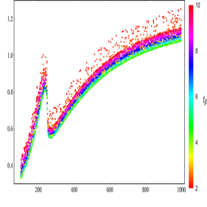
In Fig. 8, we show cross-sections for $\gamma\gamma\rightarrow hh,\leavevmode\nobreak\ HH$ in the IHDM, together with the ones for $hh$ production in the SM, as functions of center-of-mass energy (CoM, or $\sqrt{\hat{s}_{\gamma\gamma}}$ ). For the generated data, we select the following parameter space in the IHDM as $M_{H^{\pm}}=200$ GeV, $M_{H}=150$ GeV and fix $\lambda_{2}=0.8$ for all cases. We vary $350$ GeV $\leq\sqrt{\hat{s}_{\gamma\gamma}}\leq 1500$ GeV in the plots. Cross-sections are presented for $\mu_{2}^{2}=0$ GeV² on the left panel and for $200^{2}$ GeV² on the right panel, respectively. In the plots, the black line shows for cross-sections for $\gamma\gamma\rightarrow hh$ in the SM and the blue (green) line presents for $\gamma\gamma\rightarrow hh\leavevmode\nobreak\ (HH)$ in THDM, respectively.

We first comment on the results in the case of $\mu_{2}^{2}=0$ GeV². The cross-sections for $hh,\leavevmode\nobreak\ HH$ in the IHDM have peaks at $\sqrt{\hat{s}_{\gamma\gamma}}\sim 2M_{H^{\pm}}=400$ GeV. In the regions $\sqrt{\hat{s}_{\gamma\gamma}}\leq 750$ GeV, $\hat{\sigma}_{hh,HH}$ in the IHDM are larger than $\hat{\sigma}_{hh}$ in the SM. Beyond the regions of $\sqrt{\hat{s}_{\gamma\gamma}}\geq 750$ GeV, the cross-sections for $HH$ in the IHDM are suppressed in comparison with $hh$ productions in both the SM and the IHDM. It is interested in finding that the production cross-sections for $\gamma\gamma\rightarrow hh,\leavevmode\nobreak\ HH$ in the IHDM are dominant around the peaks compared with $\hat{\sigma}_{hh}$ in the SM. It indicates that the contributions from singly charged Higgs in the loop of $\gamma\gamma\rightarrow hh,\leavevmode\nobreak\ HH$ are massive attributions in the regions.

In the case of $\mu_{2}^{2}=200^{2}$ GeV², we only observe a peak of $\hat{\sigma}_{HH}$ in the IHDM around $\sqrt{\hat{s}_{\gamma\gamma}}\sim 2M_{H^{\pm}}=400$ GeV. In further, the data shows that the cross-sections for $HH$ production are dominant in the regions $\sqrt{\hat{s}_{\gamma\gamma}}\leq 750$ GeV in contrast with the corresponding ones for $hh$ productions in both the SM and the IHDM. Beyond the regions $\sqrt{\hat{s}_{\gamma\gamma}}\geq 750$ GeV, $\hat{\sigma}_{HH}$ are suppressed. It is observed that the cross-sections for $hh$ production in the IHDM are smaller than $\hat{\sigma}_{hh}$ in the SM when $\sqrt{\hat{s}_{\gamma\gamma}}\leq 550$ GeV. In the regions of $\sqrt{\hat{s}_{\gamma\gamma}}\geq 550$ GeV, $\hat{\sigma}_{hh}$ in the IHDM tend to the cross-sections for $hh$ production in the SM. This can be explained as follows. Since the $hh$ productions in the IHDM are different from the ones in the SM by the contributions of charged Higgs in the loop of triangle $h^{*}$ -pole and box diagrams. These contributions depend on $M_{H^{\pm}}$ and the vertices $hH^{\pm}H^{\mp}$ , $hhH^{\pm}H^{\mp}$ expressing in terms of $\mu_{2}^{2}$ . At the large value of $\mu_{2}^{2}$ these contributions may be cancelled out. As a result, cross-sections for $hh$ productions in the IHDM tend to the corresponding ones in the SM. Another case of $HH$ production, we have no couplings of $HH^{\pm}H^{\mp}$ due to the $Z_{2}$ -symmetry and the vertex $HHH^{\pm}H^{\mp}$ depend on $\lambda_{2}$ . Therefore, we have no such cancellations as mentioned. It is reasonable that the cross-sections for $HH$ production in the IHDM are dominant in the regions $\sqrt{\hat{s}_{\gamma\gamma}}\leq 550$ GeV and they also have peak at $\sqrt{\hat{s}_{\gamma\gamma}}\sim 2M_{H^{\pm}}=400$ GeV.

4.1.2 Enhancement factors

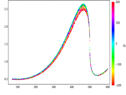
The enhancement factors given in Eq. 42 are examined in the IHDM. In Fig. 9, the factors for $\gamma\gamma\rightarrow hh,\leavevmode\nobreak\ HH$ are scanned in the parameter space of $M_{H^{\pm}},\leavevmode\nobreak\ \mu_{2}^{2}$ . In the following scatter plots, singly charged Higgs masses are varied from $70$ GeV $\leq M_{H^{\pm}}\leq 600$ GeV and $-200$ GeV $\leq\mu_{2}\leq 200$ GeV. Furthermore, we fix $\lambda_{2}=0.8$ and $M_{H}=150$ GeV for all cases. The data is generated at $\sqrt{\hat{s}_{\gamma\gamma}}=500$ (all left panel scatter-plots) GeV and at $\sqrt{\hat{s}_{\gamma\gamma}}=1000$ GeV (all right panel scatter-plots).

The factors for $hh$ productions in the IHDM are first analyzed. Since the cross-sections for $hh$ productions are enhanced around the peaks at $\sqrt{\hat{s}_{\gamma\gamma}}\sim 2M_{H^{\pm}}$ . Therefore, it is not surprised in finding that $\mu_{hh}^{\textrm{IHDM}}$ becomes largest at $\sqrt{\hat{s}_{\gamma\gamma}}\sim 2M_{H^{\pm}}=250$ GeV (for the left plots) and at $\sqrt{\hat{s}_{\gamma\gamma}}\sim 2M_{H^{\pm}}=500$ GeV (for the right plots). Around these peaks, the data indicates that the enhancement factors tend to about $\sim 1.5$ in the limit of $\mu_{2}^{2}\rightarrow M_{H^{\pm}}^{2}$ . Since the contributions of charged Higgs in the loop being small when $\mu_{2}^{2}\rightarrow M_{H^{\pm}}^{2}$ (due to the fact that the couplings of $hH^{\pm}H^{\mp}$ , $hhH^{\pm}H^{\mp}$ tend to zero in this limit). It is found that the enhancement factors can reach to factor of $6$ (for $500$ GeV of CoM) and factor of $13$ (for $1000$ GeV of CoM) around the peaks. Beyond the peaks, we observe that $1\leq\mu_{hh}^{\textrm{IHDM}}\leq 2$ .

For the enhancement factors of $HH$ productions in the IHDM, we also find $\mu_{HH}^{\textrm{IHDM}}$ becomes largest contributions at $\sqrt{\hat{s}_{\gamma\gamma}}\sim 2M_{H^{\pm}}=250$ GeV (for the left plots) and at $\sqrt{\hat{s}_{\gamma\gamma}}\sim 2M_{H^{\pm}}=500$ GeV (for the right plots). It is attentive to realize that $\mu_{HH}^{\textrm{IHDM}}$ have different behavior in comparison with $\mu_{hh}^{\textrm{IHDM}}$ . At the $500$ GeV of CoM, the factors develop to the peak and then are decreased rapidly beyond the peak. However, they grow up with the charged Higgs masses in the above regions of $M_{H^{\pm}}\geq\sim 300$ GeV. Because there aren’t couplings $HH^{\pm}H^{\mp}$ due to the $Z_{2}$ -symmetry and the vertex $HHH^{\pm}H^{\mp}$ only depends on $\lambda_{2}$ . Therefore, in the high regions of charged Higgs masses, the factors $\mu_{HH}^{\textrm{IHDM}}$ are increased with $M_{H^{\pm}}$ .

In Fig. 10, the enhancement factors for $\gamma\gamma\rightarrow hh,\leavevmode\nobreak\ HH$ are generated in the space of $M_{H^{\pm}},\leavevmode\nobreak\ \lambda_{2}$ . The charged Higgs masses are varied as $70$ GeV $\leq M_{H^{\pm}}\leq 600$ GeV and $0\leq\lambda_{2}\leq 4$ . We fix $\mu_{2}^{2}=200^{2}$ GeV² and $M_{H}=150$ GeV for all cases. In the scatter plots, we set $\sqrt{\hat{s}_{\gamma\gamma}}=500$ (for all left panel plots) GeV and $\sqrt{\hat{s}_{\gamma\gamma}}=1000$ GeV (for all right panel plots). For the factors $\mu_{hh}^{\textrm{IHDM}}$ (as shown in all the above scatter plots), both the couplings $hH^{\pm}H^{\mp}$ and $hhH^{\pm}H^{\mp}$ are independent of $\lambda_{2}$ . As a result, the factors only depend on $M_{H^{\pm}}$ . For the factors $\mu_{HH}^{\textrm{IHDM}}$ (as shown in all the below scatter plots), it is found that the quadratic-coupling $HHH^{\pm}H^{\mp}$ depend on $\lambda_{2}$ . As a result, the factors depend strongly on $\lambda_{2}$ and $M_{H^{\pm}}$ . These massive contributions are mainly from the charged Higgs exchanging in the box diagrams.

4.2 THDM

The phenomenological results for the production processes $\gamma\gamma\rightarrow\phi_{i}\phi_{j}$ with CP-even Higgses $\phi_{i,j}\equiv h,H$ in the THDM are analysed in the following subsection.

4.2.1 Production cross-sections

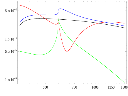
Cross-sections for $\gamma\gamma\rightarrow\phi_{i}\phi_{j}$ in the THDM are first investigated at several CoM energies. In Fig. 11, $\hat{\sigma}_{\gamma\gamma\rightarrow\phi_{i}\phi_{j}}$ in the THDM together with $\hat{\sigma}_{\gamma\gamma\rightarrow hh}$ in the SM, are presented as functions of $\sqrt{\hat{s}_{\gamma\gamma}}$ . The following data is generated at $M_{H^{\pm}}=300$ GeV, $M_{H}=150$ GeV and $t_{\beta}=5$ . The CoM energies are varied as $350$ GeV $\leq\sqrt{\hat{s}_{\gamma\gamma}}\leq 1500$ GeV in the selected-configurations. The $Z_{2}$ -breaking parameter $m_{12}^{2}=M^{2}/s_{\beta}c_{\beta}$ is selected as follows: $M^{2}=0,\leavevmode\nobreak\ 200^{2},\leavevmode\nobreak\ 500^{2},\leavevmode\nobreak\ 700^{2}$ GeV². In further, the mixing angle $\alpha$ is taken as $c_{\beta-\alpha}=+0.2$ and $s_{\beta-\alpha}=+\sqrt{1-c_{\beta-\alpha}^{2}}$ , accordingly. The notations for all lines appear in the presented plots are as follows: the black line shows for cross-sections of $\gamma\gamma\rightarrow hh$ in the SM. While the blue line presents for $\gamma\gamma\rightarrow hh$ in THDM. Additionally, the green (red) line presents for $\gamma\gamma\rightarrow hH$ ( $\gamma\gamma\rightarrow HH$ ) in THDM, respectively. Generally, we observe that $\hat{\sigma}_{\phi_{i}\phi_{j}}$ are enhanced at $\sqrt{\hat{s}_{\gamma\gamma}}\sim 2M_{H^{\pm}}=600$ GeV for all cases. Among the productions, the data shows that cross-sections for $\gamma\gamma\rightarrow hH$ are suppressed compared with other productions, as the consequences of the softly breaking the $Z_{2}$ -symmetry. However, $\hat{\sigma}_{hH}$ become more and more significant once $M^{2}$ being the large values.

We first inspect the data in the case of $M^{2}=0$ . One notices that $\hat{\sigma}_{HH}$ become largest in the regions $\sqrt{\hat{s}_{\gamma\gamma}}\leq\sim 450$ GeV and they are decreased rapidly in the regions $\sqrt{\hat{s}_{\gamma\gamma}}\geq 450$ GeV. Moreover, $\hat{\sigma}_{hh}$ in the SM and the THDM are dominant in the regions of $\sqrt{\hat{s}_{\gamma\gamma}}\geq 450$ GeV contrasted to the ones for $\gamma\gamma\rightarrow hH,\leavevmode\nobreak\ HH$ in the THDM. Among the mentioned cross-sections, the $hh$ production in the THDM is largest in this case.

When $M^{2}=200^{2}$ GeV², the cross-sections for $HH$ productions in THDM become largest in comparison with other ones. These massive contributions are attributed from charged Higgs in the loop. Due to the $Z_{2}$ -symmetry, the productions of $hH$ in the THDM are still suppressed in this case. For high regions of $M^{2}$ , taking $M^{2}=500^{2},\leavevmode\nobreak\ 700^{2}$ GeV² as examples, the productions $\gamma\gamma\rightarrow hH,\leavevmode\nobreak\ HH$ are more and more dominant in comparison with $hh$ production in the SM and in the THDM.

Fermionphobic limit

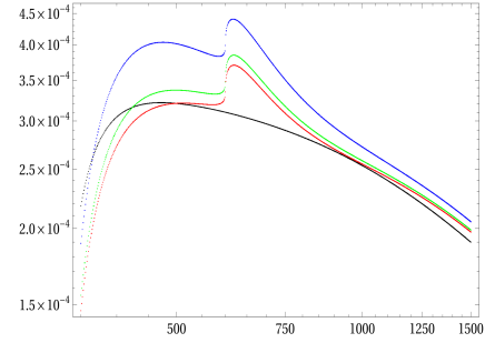
The fermionphobic limit is studied in which the mixing angle is taken as $\alpha=\pm\pi/2$ . For a typical example, we select $\alpha=+\pi/2$ in the following plots. Since, we have already checked that top quark propagating in the loop is dominant contributions versus other fermions. It is enough to take into account top quark in the loop for the present calculations. It means that the cross-sections are only contributed from $W$ boson and scalar particles in the loop when we consider the fermionphobic limit. Subsequently, we can examine the comparative sizes among these contributions. In Fig. 12 (for $hh$ production), Fig. 13 (for $hH$ production), Fig. 14 (for $HH$ production), the corresponding cross-sections for $\gamma\gamma\rightarrow\phi_{i}\phi_{j}$ in the THDM together with $\hat{\sigma}_{hh}$ in the SM as functions of $\sqrt{\hat{s}_{\gamma\gamma}}$ , are analysed in the fermionphobic limit. The CoM energies are varied $350$ GeV $\leq\sqrt{\hat{s}_{\gamma\gamma}}\leq 1500$ GeV. We select $M_{H^{\pm}}=300$ GeV and apply $t_{\beta}=3$ (blue line), $t_{\beta}=5$ (green line), $t_{\beta}=7$ (red line), respectively. Moreover, we fix $M_{H}=150$ GeV for all cases. In further, the results are presented at $M^{2}=0$ GeV² (for all the left Figures) and at $M^{2}=+200^{2}$ GeV² (for all the right Figures).

The $hh$ productions in the SM and the THDM at $M^{2}=0$ GeV² are first analysed. We notice that the cross-sections depend slightly on $t_{\beta}$ in the regions below the peak $\sqrt{\hat{s}_{\gamma\gamma}}\sim 2M_{H^{\pm}}=600$ GeV. In the regions above the peak, it is found that the cross-sections are more sensitive to $t_{\beta}$ . For the case of $M^{2}=200^{2}$ GeV², the cross-sections are proportional to $t_{\beta}$ . Around the peak regions, the cross-sections are enhanced by charged Higgs loop.

As mentioned in above, the cross-sections for $hH$ productions in the THDM are suppressed due to the softly breaking of the $Z_{2}$ -symmetry. It is explainable for cross-sections for $hH$ productions are much smaller than the corresponding ones for $hh$ productions in the SM. However, at the peak of $\sqrt{\hat{s}_{\gamma\gamma}}=2M_{H^{\pm}}=600$ GeV, the cross-sections are enhanced and can reach to order of $\hat{\sigma}_{hh}$ in the SM. At $M^{2}=0$ , $\hat{\sigma}_{\gamma\gamma\rightarrow hH}$ are more sensitive to $t_{\beta}$ in all range of CoM. Another case of $M^{2}=+200^{2}$ GeV², the cross-sections are also more sensitive to $t_{\beta}$ in the regions below the peak $\sim 600$ GeV. But they are nearly proportional to $t_{\beta}$ beyond the peak.

For all cases of $M^{2}$ in $HH$ productions, it is interested in finding that the cross-sections are larger than $\hat{\sigma}_{hh}$ in the SM and they are proportional to $1/t_{\beta}$ for all range of CoM. We also observe that cross-sections are enhanced around the peak $\sim 2M_{H^{\pm}}=600$ GeV. The dominant contributions are from the singly charged Higgs exchanging in the loop.

Decoupling limit

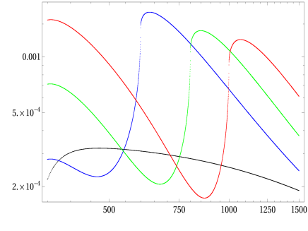
We next study the decoupling limit in which the mixing angle is taken as $\beta-\alpha=\pi/2$ . In Fig. 15 ( $hh$ production), Fig. 16 ( $hH$ production), Fig. 17 ( $HH$ production), cross-sections for $\gamma\gamma\rightarrow\phi_{i}\phi_{j}$ in the THDM together with $\gamma\gamma\rightarrow hh$ in the SM, as functions of $\sqrt{\hat{s}_{\gamma\gamma}}$ are examined in the decoupling limit. In the Figures 15, cross-sections for $hh$ productions in the decoupling limit are investigated at $M^{2}=0$ GeV² (on left panel) and at $M^{2}=200$ GeV² (on right panel). The CoM energy is varied as $350$ GeV $\leq\sqrt{\hat{s}_{\gamma\gamma}}\leq 1500$ GeV. We select $M_{\phi}=M_{H}=M_{A^{0}}=M_{H^{\pm}}=300$ GeV (blue line), $400$ GeV (green line), $500$ GeV (red line) and set $t_{\beta}=5$ for all cases. In both cases, cross-sections $\hat{\sigma}_{\gamma\gamma\rightarrow hh}$ have the peaks at $\sqrt{\hat{s}_{\gamma\gamma}}=2M_{H^{\pm}}=600,\leavevmode\nobreak\ 800,\leavevmode\nobreak\ 1000$ GeV, respectively. Furthermore, $\hat{\sigma}_{hh}$ in the THDM are larger than $\hat{\sigma}_{hh}$ in the SM. It is explained that the charged Higgs loop contributions being significant contributions once $M_{\phi}$ being large. At $M^{2}=0$ GeV², it is seem that cross-sections depend on $1/M_{\phi}$ in the regions below the peaks and are proportional to $M_{\phi}$ in the regions above the peak. When $M^{2}=200$ GeV², we find clearly that cross-sections are proportional to $M_{\phi}$ .

For the productions of $hH,\leavevmode\nobreak\ HH$ in the THDM in the decoupling limit, we emphasize that we take $M_{H}=150$ GeV and note $M_{\phi}=M_{H^{\pm}}=300,\leavevmode\nobreak\ 400,\leavevmode\nobreak\ 500$ GeV in these cases. Other parameters are set as in the previous case. It is not surprised that the cross-sections for $hH$ in the THDM are suppressed because of breaking of the $Z_{2}$ -symmetry. For the $HH$ productions at $M^{2}=0$ , the cross-sections are greater than the $hh$ productions in the SM in the below of the peak regions. But they are decreased rapidly and become smaller than the ones for $hh$ productions in the SM. For the $HH$ productions at $M^{2}=200$ GeV², the cross-sections are greater than $\hat{\sigma}_{hh}$ in the SM for most of CoM.

4.2.2 Enhancement factors

We pay attention to investigate the enhancement factors defined in Eq. 42 for $\gamma\gamma\rightarrow\phi_{i}\phi_{j}$ in the THDM. The factors scanned over parameter space of $M_{H^{\pm}},\leavevmode\nobreak\ t_{\beta}$ are first studied in this subsection. Two scenarios for $c_{\beta-\alpha}>0$ and $c_{\beta-\alpha}<0$ are examined in detail. In Figs. 18, 19, we fix $M^{2}=M_{H}^{2}=200^{2}$ GeV². Moreover, we vary $100$ GeV $\leq M_{H^{\pm}}\leq 1000$ GeV and set $2\leq t_{\beta}\leq 10$ in the following plots. The factors $\mu_{\phi_{i}\phi_{j}}^{\textrm{THDM}}$ are generated at $\sqrt{\hat{s}_{\gamma\gamma}}=500$ GeV (for all above scatter-plots) and examined at $\sqrt{\hat{s}_{\gamma\gamma}}=1000$ GeV (for all below scatter-plots). In the left panel, we show for the enhancement factors for $hh$ productions. In the middle (right) panel, the enhancement factors for $hH,\leavevmode\nobreak\ (HH)$ productions are presented, respectively.

In Fig. 18, the first scenario for $c_{\beta-\alpha}>0$ is explored. In this scenario, we take $c_{\beta-\alpha}=+0.2$ for an example and $s_{\beta-\alpha}=+\sqrt{1-c_{\beta-\alpha}^{2}}$ , correspondingly. At $\sqrt{\hat{s}_{\gamma\gamma}}=500$ GeV, $\mu_{hh}^{\textrm{THDM}}$ change from $1$ to $1.5$ for all range of $M_{H^{\pm}}$ . The values of $\mu_{hh}^{\textrm{THDM}}$ are enhanced around the peak at $M_{H^{\pm}}=\sqrt{\hat{s}_{\gamma\gamma}}/2=250$ GeV. Predominantly, the factors are proportional to $t_{\beta}^{-1}$ in this case. Interestingly, we observe that the factors $\mu_{hH}^{\textrm{THDM}}$ change from $0$ to $0.5$ for all range of $M_{H^{\pm}}$ . The suppressed values of $\mu_{hH}^{\textrm{THDM}}$ are expected as explained in previous paragraphs due to the $Z_{2}$ -symmetry. The $\mu_{hH}^{\textrm{THDM}}$ are the same behavior as $\mu_{hh}^{\textrm{THDM}}$ which they are inversely proportional to $t_{\beta}$ . In the other hand, the enhancement factors for $HH$ productions in the THDM are strongly dependent of the charged Higgs mass but change slightly with $t_{\beta}$ . In all range of $M_{H^{\pm}}$ , the factors $\mu_{HH}^{\textrm{THDM}}$ are from $0.3$ to $1.2$ .

At $\sqrt{\hat{s}_{\gamma\gamma}}=1000$ GeV, the factors $\mu_{hh}^{\textrm{THDM}}$ become biggest at the peak at $M_{H}^{\pm}=\sqrt{\hat{s}_{\gamma\gamma}}/2=500$ GeV. Around the peak, $\mu_{hh}^{\textrm{THDM}}$ change from $1.2$ to $1.8$ . Beyond the peak, the factors are changed from $1.0$ to $1.2$ in all range of $M_{H^{\pm}}$ . It is stress that $\mu_{hh}^{\textrm{THDM}}$ slightly change with $t_{\beta}$ . For $HH$ productions, $\mu_{HH}^{\textrm{THDM}}$ are varied from $0.4$ to $2.5$ around the peak (at $M_{H^{\pm}}=500$ GeV) regions. It is realized that $\mu_{HH}^{\textrm{THDM}}$ slightly change with $t_{\beta}$ . Otherwise, $\mu_{hH}^{\textrm{THDM}}$ are much smaller than $1$ and are inversely proportional to $t_{\beta}$ .

Another scenario for $c_{\beta-\alpha}<0$ is considered for examining how are the factors effect by setting different sign of $c_{\beta-\alpha}$ in this work. In Fig. 19, we take $c_{\beta-\alpha}=-0.2$ for an example and $s_{\beta-\alpha}=+\sqrt{1-c_{\beta-\alpha}^{2}}$ , accordingly. At $\sqrt{\hat{s}_{\gamma\gamma}}=500$ GeV, it is excited in observing that $\mu_{hh}^{\textrm{THDM}}$ are different behavior in comparison with previous scenario. At this CoM energy, the factors $\mu_{hh}^{\textrm{THDM}}$ can reach to $1.5$ in the low region of $M_{H^{\pm}}<200$ GeV. They then are decreased to around $0.9$ when $M_{H^{\pm}}>200$ GeV. There isn’t peak of the factors observed in this scenario. Because the contributions of singly charged Higgs exchanging in the one-loop triangle diagrams may cancel out with the ones one-loop box diagrams in this scenario. Surprisingly, we find that the factors $\mu_{hh}^{\textrm{THDM}}$ are proportional to $t_{\beta}$ in this scenario. For the $hH$ productions, the factors are suppressed and they are in the range of $[\sim 0.025,\sim 0.3]$ . They are sensitive with $t_{\beta}^{-1}$ in all range of charged Higgs mass. In $HH$ productions, it is found that the factors develop to the peak around $M_{H^{\pm}}=500$ GeV. They reach to factor $2.5$ around the peak and they are in the ranges of $[\sim 0.5,\sim 1.7]$ beyond the peak regions. In all range of $M_{H^{\pm}}$ , the factors $\mu_{HH}^{\textrm{THDM}}$ are proportional to $t_{\beta}^{-1}$ in this scenario.

The survey for all the enhancement factors at $\sqrt{\hat{s}_{\gamma\gamma}}=1000$ GeV are concerned in the next paragraphs. The factors $\mu_{hh}^{\textrm{THDM}}$ are large in the regions ( $M_{H^{\pm}}\leq 200$ GeV) and they can reach to $1.5$ . They then are decreased rapidly to the regions around $M_{H^{\pm}}\sim 300$ GeV and develop to the peak at $M_{H^{\pm}}=\sqrt{\hat{s}_{\gamma\gamma}}/2=500$ GeV. Around the peak, the enhancement factor is about $1.2$ . In other ranges of charged Higgs mass, $\mu_{hh}^{\textrm{THDM}}\sim 0.9$ . One also finds that $\mu_{hh}^{\textrm{THDM}}$ is inversely proportional to $t_{\beta}$ in this scenario. In $hH$ productions, the factors are increased to the peak $M_{H^{\pm}}=\sqrt{\hat{s}_{\gamma\gamma}}/2=500$ GeV and they are about $0.3$ around the peak. In all regions of $M_{H^{\pm}}$ , the mentioned factors are in the ranges of $[\sim 0.025,\sim 0.3]$ and they are inversely proportional to $t_{\beta}$ . In the last case, it is found that the factors $\mu_{HH}^{\textrm{THDM}}$ are same behavior as previous scenario. They are in the ranges of $[\sim 0.5,\sim 4]$ in all regions of $M_{H^{\pm}}$ . However, the factors $\mu_{HH}^{\textrm{THDM}}$ depend slightly on $t_{\beta}$ in this scenario.

The enhancement factors scanned over the parameter space of $M_{H^{\pm}},\leavevmode\nobreak\ M^{2}$ in the THDM are also interested greatly in this work. Two scenarios for $c_{\beta-\alpha}>0$ and $c_{\beta-\alpha}<0$ are studied in detail in the following paragraphs. In Fig. 20 (for $c_{\beta-\alpha}>0$ scenario), Fig. 21 (for $c_{\beta-\alpha}<0$ scenario), we consider $\sqrt{\hat{s}_{\gamma\gamma}}=500$ GeV (for all the above scatter plots) and $\sqrt{\hat{s}_{\gamma\gamma}}=1000$ GeV (for all the below scatter plots). Moreover, we vary charged Higgs mass as $100$ GeV $\leq M_{H^{\pm}}\leq 1000$ GeV, the soft-breaking parameter as $0$ GeV² $\leq M^{2}\leq 200^{2}$ GeV² and take $t_{\beta}=5$ for all cases.

In Fig. 20, the first scenario of $c_{\beta-\alpha}>0$ is examined. For this case, we take $c_{\beta-\alpha}=+0.2$ as an example and $s_{\beta-\alpha}=+\sqrt{1-c_{\beta-\alpha}^{2}}$ , accordingly. For $hh$ production at $\sqrt{\hat{s}_{\gamma\gamma}}=500$ GeV, we observe the peak of $\mu_{hh}^{\textrm{THDM}}$ at $M_{H^{\pm}}=250$ GeV which is corresponding to the threshold of cross-sections $hh$ in the THDM at the peak $\sqrt{\hat{s}_{\gamma\gamma}}=2M_{H^{\pm}}$ . Around the peak, $\mu_{hh}^{\textrm{THDM}}$ are varied from $1.0$ to $1.8$ . Above the peak regions, the enhancement factors tend to $1.2$ and depend slightly on $M^{2}$ . For $hH$ productions, $\mu_{hH}^{\textrm{THDM}}$ are more sensitive with $M^{2}$ in below the peak regions. The factors are in the ranges of $[0.07,1.5]$ in above the peak regions. Around the peak, $\mu_{hH}^{\textrm{THDM}}$ can reach to $0.3$ . We also find the same behavior for $\mu_{HH}^{\textrm{THDM}}$ . The factors for $HH$ productions are large in the low regions of $M_{H^{\pm}}$ and around the peak $M_{H^{\pm}}=250$ GeV. They are in the ranges of $[0.7,2.4]$ in the above the peak regions. Generally, we observe that $\mu_{\phi_{i}\phi_{j}}^{\textrm{THDM}}$ are proportional to $1/M$ at this CoM energy.

At $\sqrt{\hat{s}_{\gamma\gamma}}=1000$ GeV, we also find that $\mu_{hh}^{\textrm{THDM}}$ develop to the peak at $M_{H^{\pm}}=500$ GeV where the factors can reach to $2.2$ and are decreased rapidly beyond the peak. The factors depend slightly on $M^{2}$ and tend to $1$ beyond the peak regions. For $hH$ productions, $\mu_{hH}^{\textrm{THDM}}$ are sensitive with $M^{2}$ in the peak regions. They tend to $0.05$ and they are slightly dependent of $M^{2}$ in the above the peak regions. For $HH$ productions, the factors become large in the below the peak regions and they are inversely proportional to $M^{-1}$ . Around the peak, the factors are enhanced by large values of $M^{2}$ . Above the peak regions, $\mu_{HH}^{\textrm{THDM}}$ are varied around $1.0$ .

Another scenario for $c_{\beta-\alpha}=-0.2<0$ is also concerned interestingly in this work. In Fig. 21, $s_{\beta-\alpha}=+\sqrt{1-c_{\beta-\alpha}^{2}}$ is obtained accordingly. We are going to comment on physical results at $\sqrt{\hat{s}_{\gamma\gamma}}=500$ GeV. For $hh$ productions, we observe different behavior of $\mu_{hh}^{\textrm{THDM}}$ in comparison with the $c_{\beta-\alpha}>0$ scenario. In concrete, the factors are large in below the peak regions. Around the peak regions, they are enhanced by the small value of $M$ and can reach to $1.6$ . Above the peak regions, the factors are in the ranges of $[0.9,1.1]$ . We also observe the different behavior for the factors in $hH$ productions compared with the previous scenario. The factors $\mu_{hH}^{\textrm{THDM}}$ get the large values in the below and around the peak regions and they are proportional to $M$ . The factors $\mu_{hH}^{\textrm{THDM}}$ are in the ranges of $[0.2,0.6]$ for $M_{H\pm}$ in above the peak regions. In the case of $HH$ productions, $\mu_{HH}^{\textrm{THDM}}$ develop to the peak at $M_{H^{\pm}}\sim 250$ GeV. They are in the range of $[1.0,\leavevmode\nobreak\ 2.4]$ in above the peak regions. In general, the factors $\mu_{HH}^{\textrm{THDM}}$ depend slightly on charged Higgs mass and are proportional to $1/M$ in above the peak regions.

We next comment on physical results at $\sqrt{\hat{s}_{\gamma\gamma}}=1000$ GeV. The factors $\mu_{hh}^{\textrm{THDM}}$ are enhanced by the small values of $M$ in low regions of charged Higgs mass and they can reach $1.2$ . They tend to $2.5$ around the peak. The factors are then varied around $\sim 0.9$ . In general, the factors depend on $M^{-1}$ . In the productions $hH$ , $\mu_{hH}^{\textrm{THDM}}$ are more sensitive to $M^{-1}$ around the peak regions. They then tend to $0.2$ in the high mass regions of singly charged Higgs. For $HH$ productions, the factors $\mu_{HH}^{\textrm{THDM}}$ strongly depend on $M^{-1}$ . At the peak, the factors are enhanced by the large value of $M$ . Above the peak regions, $\mu_{HH}^{\textrm{THDM}}$ tend to $\sim 1$ .

5 Conclusions

In this paper, we have presented the results for one-loop induced processes $\gamma\gamma\rightarrow\phi_{i}\phi_{j}$ with CP-even Higgses $\phi_{i,j}\equiv h,\leavevmode\nobreak\ H$ at high energy photon-photon collision in the IHDM and the THDM. In the phenomenological results, we have shown the cross-sections at several center-of-mass energies. The results show that cross-sections for the computed processes in the models under investigations are enhanced at around the threshold of charged Higgs pair ( $\sim 2M_{H^{\pm}}$ ). Furthermore, the enhancement factors for the processes are examined in parameter space of the models under consideration. In the IHDM, the factors are studied in the parameter space of $(M_{H^{\pm}},\leavevmode\nobreak\ \mu^{2}_{2})$ and $(M_{H^{\pm}},\leavevmode\nobreak\ \lambda_{2})$ . In the the THDM, the factors are analysed in the planes of $(M_{H^{\pm}},\leavevmode\nobreak\ t_{\beta})$ and $(M_{H^{\pm}},\leavevmode\nobreak\ M^{2})$ . Two scenarios of $c_{\beta-\alpha}>0$ and $c_{\beta-\alpha}<0$ have studied in further detail. The factors give a different behavior from considering these scenarios. As a result, discriminations for the above-mentioned scenarios can be performed at future colliders.

Acknowledgment: This research is funded by Vietnam National Foundation for Science and Technology Development (NAFOSTED) under the grant number $103.01$ - $2023.16$ .

Appendix A: Effective Lagrangian in the IHDM

The kinematic terms of Lagrangian in the IHDM can be expanded as follows:

$\displaystyle\mathcal{L}_{K}^{\text{IHDM}}$	$\displaystyle\supset$	$\displaystyle\frac{2M_{W}^{2}}{v}W^{\pm}_{\mu}W^{\mp,\mu}h+\frac{M_{Z}^{2}}{v}hZ_{\mu}Z^{\mu}+i\frac{M_{Z}c_{2W}}{v}Z^{\mu}(H^{\mp}\partial_{\mu}H^{\pm}-H^{\pm}\partial_{\mu}H^{\mp})$	(43)
		$\displaystyle+i\frac{M_{Z}s_{2W}}{v}A^{\mu}(H^{\mp}\partial_{\mu}H^{\pm}-H^{\pm}\partial_{\mu}H^{\mp})+i\frac{2M_{Z}^{2}c_{W}^{2}s_{W}}{v}A^{\mu}W_{\mu}^{\pm}G^{\pm}$
		$\displaystyle+i\frac{M_{W}}{v}(HW^{\mp,\mu}\partial_{\mu}H^{\pm}-H^{\pm}W^{\mp,\mu}\partial_{\mu}H-HW^{\pm}_{\mu}\partial^{\mu}H^{\mp}+H^{\mp}W^{\pm}_{\mu}\partial^{\mu}H)$
		$\displaystyle+\frac{M_{Z}^{2}s_{2W}^{2}}{v^{2}}A_{\mu}A^{\mu}H^{\pm}H^{\mp}+\frac{2M_{Z}^{2}c_{W}^{2}s_{W}}{v^{2}}HH^{\pm}W_{\mu}^{\mp}A^{\mu}+\frac{2M_{W}^{2}}{v^{2}}W^{\pm}_{\mu}W^{\mp,\mu}hh$
		$\displaystyle+\frac{2M_{W}^{2}}{v^{2}}W^{\pm}_{\mu}W^{\mp,\mu}HH+\frac{M_{Z}^{2}s_{2W}^{2}}{v^{2}}A_{\mu}A^{\mu}G^{\pm}G^{\mp}$
		$\displaystyle+i\frac{M_{Z}s_{2W}}{v}A^{\mu}(G^{\mp}\partial_{\mu}G^{\pm}-G^{\pm}\partial_{\mu}G^{\mp})+\cdots.$

We also expand the scalar Higgs potential of the IHDM and collect the terms involving to Higgs self-coupling as follows:

$\displaystyle-\mathcal{V}_{\text{IHDM}}(\phi_{1},\phi_{2})$	$\displaystyle\supset$	$\displaystyle-\frac{3M_{h}^{2}}{v}hhh+\frac{2(\mu_{2}^{2}-M_{H}^{2})}{v}hHH+\frac{2(\mu_{2}^{2}-M_{H^{\pm}}^{2})}{v}hH^{\pm}H^{\mp}$	(44)
		$\displaystyle+\frac{M_{H^{\pm}}^{2}-M_{H}^{2}}{v}HH^{\pm}{G^{\mp}}+\frac{2(\mu_{2}^{2}-M_{H^{\pm}}^{2})}{v^{2}}hhH^{\pm}H^{\mp}-2\lambda_{2}HHH^{\pm}H^{\mp}$
		$\displaystyle-\frac{M_{h}^{2}}{v^{2}}hhG^{\pm}G^{\mp}+\frac{2(\mu_{2}^{2}-M_{H^{\pm}}^{2})}{v^{2}}HHG^{\pm}G^{\mp}+\cdots.$

Appendix B: Effective Lagrangian in the THDM

We expand the kinematic terms of Lagrangian in the THDM as follows:

$\displaystyle\mathcal{L}_{K}^{\text{THDM}}$	$\displaystyle\supset$	$\displaystyle\frac{2M_{W}^{2}}{v}s_{\beta-\alpha}hW_{\mu}^{\pm}W^{\mp,\mu}+\frac{2M_{W}^{2}}{v}c_{\alpha-\beta}HW_{\mu}^{\pm}W^{\mp,\mu}+\frac{M_{Z}^{2}}{v}s_{\beta-\alpha}hZ_{\mu}Z^{\mu}$	(45)
		$\displaystyle+\frac{M_{Z}^{2}}{v}c_{\alpha-\beta}HZ_{\mu}Z^{\mu}+i\frac{M_{Z}c_{2W}}{v}Z^{\mu}(H^{\mp}\partial_{\mu}{H^{\pm}}-H^{\pm}\partial_{\mu}H^{\mp})$
		$\displaystyle+i\frac{M_{Z}s_{2W}}{v}A^{\mu}(H^{\mp}\partial_{\mu}{H^{\pm}}-H^{\pm}\partial_{\mu}H^{\mp})+\frac{4M_{W}^{2}s_{W}^{2}}{v^{2}}H^{\pm}H^{\mp}A_{\mu}{A^{\mu}}$
		$\displaystyle-i\frac{M_{W}s_{\beta-\alpha}}{v}(HW^{\mp,\mu}\partial_{\mu}H^{\pm}-HW^{\pm,\mu}\partial_{\mu}H^{\mp}+H^{\mp}W^{\pm,\mu}\partial_{\mu}H-H^{\pm}W^{\mp,\mu}\partial_{\mu}H)$
		$\displaystyle-i\frac{M_{W}c_{\beta-\alpha}}{v}(-hW^{\mp,\mu}\partial_{\mu}H^{\pm}+hW^{\pm,\mu}\partial_{\mu}H^{\mp}-H^{\mp}W^{\pm,\mu}\partial_{\mu}h+H^{\pm}W^{\mp,\mu}\partial_{\mu}h)$
		$\displaystyle+\frac{2M_{W}^{2}s_{W}c_{\beta-\alpha}}{v^{2}}hH^{\mp}W_{\mu}^{\pm}A^{\mu}-\frac{2M_{W}^{2}s_{W}s_{\beta-\alpha}}{v^{2}}HH^{\mp}W^{\pm}_{\mu}A^{\mu}$
		$\displaystyle+\dfrac{2M_{W}^{2}}{v^{2}}W^{\pm}_{\mu}W^{\mp,\mu}HH+\frac{2M_{W}^{2}}{v^{2}}W^{\pm}_{\mu}W^{\mp,\mu}hh+\cdots$

Expanding the scalar potential in the THDM, we then collect the terms involving to the Higgs self-couplings as

	$\displaystyle-\mathcal{V}_{\text{THDM}}(\phi_{1},\phi_{2})$	$\displaystyle\supset$	$\displaystyle-\lambda_{hHH}hHH-\lambda_{Hhh}Hhh-\lambda_{hH^{\pm}H^{\mp}}hH^{\pm}H^{\mp}$		(46)
			$\displaystyle-\lambda_{hH^{\pm}H^{\mp}}HH^{\pm}H^{\mp}-\lambda_{HhH^{\pm}H^{\mp}}HhH^{\pm}H^{\mp}+\cdots.$		(46)

All coefficients of the mentioned couplings are shown explicitly in terms of physical parameters as follows:

$\displaystyle-\lambda_{hHH}$	$\displaystyle=$	$\displaystyle\frac{3\lambda_{1}v}{2}s_{\alpha}c_{\alpha}^{2}c_{\beta}-\frac{3\lambda_{2}v}{2}s_{\beta}s_{\alpha}^{2}c_{\alpha}-\frac{\lambda_{345}}{2}v[c_{\beta}(2s_{\alpha}c_{\alpha}^{2}-s_{\alpha}^{3})+s_{\beta}(c_{\alpha}^{3}-2s_{\alpha}^{2}c_{\alpha})]$	(47)
	$\displaystyle=$	$\displaystyle\frac{s_{\alpha-\beta}[s_{2\alpha}(3M^{2}-M_{h}^{2}-2M_{H}^{2})+M^{2}s_{2\beta}]}{v\;s_{2\beta}},$	(48)
$\displaystyle-\lambda_{Hhh}$	$\displaystyle=$	$\displaystyle-\frac{3\lambda_{1}v}{2}c_{\beta}c_{\alpha}s_{\alpha}^{2}-\frac{3\lambda_{2}v}{2}s_{\beta}c_{\alpha}^{2}s_{\alpha}-\frac{\lambda_{345}}{2}v[s_{\beta}(s_{\alpha}^{3}-2c_{\alpha}^{2}s_{\alpha})-c_{\beta}(2c_{\alpha}s_{\alpha}^{2}-c_{\alpha}^{3})]$	(49)
	$\displaystyle=$	$\displaystyle\frac{c_{\alpha-\beta}[s_{2\alpha}(3M^{2}-M_{H}^{2}-2m_{h}^{2})-M^{2}s_{2\beta}]}{v\;s_{2\beta}},$	(50)
$\displaystyle-\lambda_{HH^{\pm}H^{\mp}}$	$\displaystyle=$	$\displaystyle-\lambda_{1}vc_{\beta}c_{\alpha}s_{\beta}^{2}-\lambda_{2}vs_{\beta}s_{\alpha}c_{\beta}^{2}-\lambda_{3}v(s_{\beta}s_{\alpha}s_{\beta}^{2}+c_{\beta}c_{\alpha}c_{\beta}^{2})+\frac{\lambda_{45}}{2}vs_{(2\beta)}\;s_{\beta+\alpha}$	(51)
	$\displaystyle=$	$\displaystyle\frac{s_{\alpha+\beta}(4M^{2}-3M_{H}^{2}-2M_{H^{\pm}}^{2})+(2M_{H^{\pm}}^{2}-M_{H}^{2})s_{\alpha-3\beta}}{2vs_{(2\beta)}},$	(52)
$\displaystyle-\lambda_{hH^{\pm}H^{\mp}}$	$\displaystyle=$	$\displaystyle\lambda_{1}vc_{\beta}s_{\alpha}s_{\beta}^{2}-\lambda_{2}vs_{\beta}c_{\alpha}c_{\beta}^{2}-\lambda_{3}v(s_{\beta}c_{\alpha}s_{\beta}^{2}-c_{\beta}s_{\alpha}c_{\beta}^{2})+\frac{\lambda_{45}}{2}v\;s_{(2\beta)}\;c_{(\beta+\alpha)}$	(53)
	$\displaystyle=$	$\displaystyle\frac{c_{\alpha+\beta}(4M^{2}-3M_{h}^{2}-2M_{H^{\pm}}^{2})+(2M_{H^{\pm}}^{2}-M_{h}^{2})c_{(\alpha-3\beta)}}{2vs_{2\beta}},$	(54)

and

$\displaystyle-\lambda_{HhH^{\pm}H^{\mp}}$	$\displaystyle=$	$\displaystyle\lambda_{1}s_{\beta}^{2}s_{\alpha}c_{\alpha}-\lambda_{2}c_{\beta}^{2}s_{\alpha}c_{\alpha}+\lambda_{3}s_{\alpha}c_{\alpha}c_{2\beta}+(\lambda_{4}+\lambda_{5})s_{\beta}c_{\beta}c_{2\alpha}$	(56)
	$\displaystyle=$	$\displaystyle\frac{s_{2\alpha}(3c_{2\alpha}+c_{2(\alpha-2\beta)}-4c_{2\beta})}{4v^{2}s_{2\beta}^{2}}M_{H}^{2}-\frac{s_{2\alpha}(3c_{2\alpha}+c_{2(\alpha-2\beta)}+4c_{2\beta})}{4v^{2}s_{2\beta}^{2}}M_{h}^{2}$
		$\displaystyle+\frac{s_{2(\alpha-\beta)}}{v^{2}}M_{H^{\pm}}^{2}+\frac{(s_{2(\alpha-3\beta)}+2s_{2(\alpha-\beta)}+5s_{2(\alpha+\beta)})}{4v^{2}s_{2\beta}^{2}}M^{2},$
$\displaystyle-\lambda_{HhG^{\pm}G^{\mp}}$	$\displaystyle=$	$\displaystyle\lambda_{1}c_{\beta}^{2}s_{\alpha}c_{\alpha}-\lambda_{2}s_{\beta}^{2}s_{\alpha}c_{\alpha}-\lambda_{3}s_{\alpha}c_{\alpha}c_{2\beta}-(\lambda_{4}+\lambda_{5})s_{\beta}c_{\beta}c_{2\alpha}$
	$\displaystyle=$	$\displaystyle\frac{1}{2v^{2}s_{2\beta}}s_{2(\alpha-\beta)}[(M_{h}^{2}-M_{H}^{2})s_{2\alpha}+2(M^{2}-M_{H^{\pm}}^{2})s_{2\beta}].$	(57)

Furthermore, we have the following couplings:

	$\displaystyle-\lambda_{hhh}$	$\displaystyle=$	$\displaystyle 3v\Big{[}\lambda_{1}s_{\alpha}^{3}c_{\beta}-\lambda_{2}c_{\alpha}^{3}s_{\beta}+(\lambda_{3}+\lambda_{4}+\lambda_{5})(s_{\alpha}c_{\beta}c_{\alpha}^{2}-c_{\alpha}s_{\beta}s_{\alpha}^{2})\Big{]}$		(58)
		$\displaystyle=$	$\displaystyle\dfrac{3e}{4M_{W}s_{W}s_{2\beta}}\Big{[}M^{2}c_{\alpha-3\beta}+(M^{2}-M_{h}^{2})c_{3\alpha-\beta}+(2M^{2}-3M_{h}^{2})c_{\alpha+\beta}\Big{]},$		(58)

	$\displaystyle-\lambda_{HHH}$	$\displaystyle=$	$\displaystyle-3v\Big{[}\lambda_{1}c_{\alpha}^{3}c_{\beta}+\lambda_{2}s_{\alpha}^{3}s_{\beta}+(\lambda_{3}+\lambda_{4}+\lambda_{5})(c_{\alpha}c_{\beta}s_{\alpha}^{2}+s_{\alpha}s_{\beta}c_{\alpha}^{2})\Big{]}$		(59)
		$\displaystyle=$	$\displaystyle\dfrac{3e}{4M_{W}s_{W}s_{2\beta}}\Big{[}M^{2}s_{\alpha-3\beta}+(M_{H}^{2}-M^{2})s_{3\alpha-\beta}+(2M^{2}-3M_{H}^{2})s_{\alpha+\beta}\Big{]},$		(59)

$\displaystyle-\lambda_{HHH^{\pm}{H^{\mp}}}$	$\displaystyle=$	$\displaystyle-\lambda_{1}c_{\alpha}^{2}s_{\beta}^{2}-\lambda_{2}s_{\alpha}^{2}c_{\beta}^{2}-\lambda_{3}(c_{\alpha}^{2}c_{\beta}^{2}+s_{\alpha}^{2}s_{\beta}^{2})+(\lambda_{4}+\lambda_{5})c_{\alpha}s_{\alpha}s_{2\beta}$	(60)
	$\displaystyle=$	$\displaystyle-\dfrac{2c_{\alpha-\beta}^{2}}{v^{2}}M_{H^{\pm}}^{2}-\frac{s_{2\alpha}[3s_{2\alpha}+s_{2(\alpha-2\beta)}-2s_{2\beta}]}{4v^{2}s_{2\beta}^{2}}M_{h}^{2}$
		$\displaystyle-\dfrac{[c_{\alpha}^{4}+c_{\alpha}^{3}s_{\alpha}\cot^{3}\beta+c_{\alpha}s_{\alpha}^{3}\cot\beta+s_{\alpha}^{4}\cot^{4}\beta]\tan^{2}\beta}{v^{2}}M_{H}^{2}$
		$\displaystyle+\dfrac{s_{\beta}[4c_{\alpha}c_{\beta}s_{\alpha}+(1+\cot^{4}\beta)s_{\alpha}^{2}s_{\beta}+c_{\alpha}^{2}(1+\cot^{4}\beta)s_{\beta}\tan^{2}\beta]}{v^{2}}M^{2},$

$\displaystyle-\lambda_{hhH^{\pm}H^{\mp}}$	$\displaystyle=$	$\displaystyle-\lambda_{1}s_{\alpha}^{2}s_{\beta}^{2}-\lambda_{2}c_{\alpha}^{2}c_{\beta}^{2}-\lambda_{3}(s_{\alpha}^{2}c_{\beta}^{2}+c_{\alpha}^{2}s_{\beta}^{2})-(\lambda_{4}+\lambda_{5})c_{\alpha}s_{\alpha}s_{2\beta}$	(61)
	$\displaystyle=$	$\displaystyle-\dfrac{2s_{\alpha-\beta}^{2}}{v^{2}}M_{H^{\pm}}^{2}-\dfrac{s_{2\alpha}[3s_{2\alpha}+s_{2(\alpha-2\beta)}+2s_{2\beta}]}{4v^{2}s_{2\beta}^{2}}M_{H}^{2}$
		$\displaystyle+\dfrac{(-c_{\alpha}^{4}\cot^{2}{\beta}+c_{\alpha}s_{\alpha}^{3}\cot\beta+c_{\alpha}^{3}s_{\alpha}\tan\beta-s_{\alpha}^{4}\tan^{2}\beta)}{v^{2}}M_{h}^{2}$
		$\displaystyle+\dfrac{s_{\beta}c_{\beta}[-4c_{\alpha}s_{\alpha}+(1+\cot^{4}\beta)s_{\alpha}^{2}\tan^{3}{\beta}+c_{\alpha}^{2}(\cot^{3}\beta+\tan\beta)]}{v^{2}}M^{2},$

	$\displaystyle-\lambda_{hhG^{\pm}G^{\mp}}$	$\displaystyle=$	$\displaystyle-\lambda_{1}s_{\alpha}^{2}c_{\beta}^{2}-\lambda_{2}c_{\alpha}^{2}s_{\beta}^{2}-\lambda_{3}(c_{\alpha}^{2}c_{\beta}^{2}+s_{\alpha}^{2}s_{\beta}^{2})+(\lambda_{4}+\lambda_{5})c_{\alpha}s_{\alpha}s_{2\beta}$		(62)
		$\displaystyle=$	$\displaystyle\dfrac{2c_{\alpha-\beta}^{2}}{v^{2}}(M^{2}-M_{H^{\pm}}^{2})-\dfrac{c_{\alpha-\beta}^{2}s_{2\alpha}}{v^{2}s_{2\beta}}M_{H}^{2}+\dfrac{-3s_{2\beta}+2s_{2\alpha}+s_{4\alpha-2\beta}}{4v^{2}s_{2\beta}}M_{h}^{2},$		(62)

	$\displaystyle-\lambda_{HHG^{\pm}G^{\mp}}$	$\displaystyle=$	$\displaystyle-\lambda_{1}c_{\alpha}^{2}c_{\beta}^{2}-\lambda_{2}s_{\alpha}^{2}s_{\beta}^{2}-\lambda_{3}(s_{\alpha}^{2}c_{\beta}^{2}+c_{\alpha}^{2}s_{\beta}^{2})-(\lambda_{4}+\lambda_{5})c_{\alpha}s_{\alpha}s_{2\beta}$		(63)
		$\displaystyle=$	$\displaystyle\dfrac{2s_{\alpha-\beta}^{2}}{v^{2}}(M^{2}-M_{H^{\pm}}^{2})+\dfrac{s_{\alpha-\beta}^{2}s_{2\alpha}}{v^{2}s_{2\beta}}M_{h}^{2}+\dfrac{-3s_{2\beta}-2s_{2\alpha}+s_{4\alpha-2\beta}}{4v^{2}s_{2\beta}}M_{H}^{2}.$		(63)

Additionally, we also derive the couplings relating to Goldstone bosons as follows:

	$\displaystyle\mathcal{L}_{K}^{\text{THDM}}$	$\displaystyle\supset$	$\displaystyle\frac{2M_{W}^{2}s_{W}}{v}A_{\mu}W^{\pm,\mu}G^{\mp}+\frac{4M_{W}^{2}s_{W}^{2}}{v^{2}}A_{\mu}A^{\mu}G^{\pm}{G^{\mp}}$		(64)
			$\displaystyle+i\frac{2M_{W}s_{W}}{v}A^{\mu}(G^{\mp}\partial_{\mu}G^{\pm}-G^{\pm}\partial_{\mu}G^{\mp})+\cdots$		(64)

From scalar potential, we have

\displaystyle-\mathcal{V}(\phi_{1},\phi_{2})

\displaystyle\supset

\displaystyle-\lambda_{hH^{\pm}G^{\mp}}hH^{\pm}G^{\mp}-\lambda_{HH^{\pm}G^{\mp}}HH^{\pm}G^{\mp}+\cdots

(65)

where the coefficients of the couplings are given by

	$\displaystyle-\lambda_{hH^{\pm}G^{\mp}}$	$\displaystyle=$	$\displaystyle\frac{ec_{\alpha-\beta}}{2M_{W}s_{W}}(M_{H^{\pm}}^{2}-M_{h}^{2}),$		(66)
	$\displaystyle-\lambda_{HH^{\pm}G^{\mp}}$	$\displaystyle=$	$\displaystyle\frac{es_{\alpha-\beta}}{2M_{W}s_{W}}(M_{H^{\pm}}^{2}-M_{H}^{2}).$		(67)

References

[1] G. Aad et al. [ATLAS], Phys. Rev. D 106 (2022) no.5, 052001 doi:10.1103/PhysRevD.106.052001 [arXiv:2112.11876 [hep-ex]].
[2] G. Aad et al. [ATLAS], Phys. Rev. Lett. 114 (2015) no.8, 081802 doi:10.1103/PhysRevLett.114.081802 [arXiv:1406.5053 [hep-ex]].
[3] G. Aad et al. [ATLAS], Eur. Phys. J. C 75 (2015) no.9, 412 doi:10.1140/epjc/s10052-015-3628-x [arXiv:1506.00285 [hep-ex]].
[4] G. Aad et al. [ATLAS], Phys. Rev. D 92 (2015), 092004 doi:10.1103/PhysRevD.92.092004 [arXiv:1509.04670 [hep-ex]].
[5] A. M. Sirunyan et al. [CMS], JHEP 01 (2018), 054 doi:10.1007/JHEP01(2018)054 [arXiv:1708.04188 [hep-ex]].
[6] M. Aaboud et al. [ATLAS], JHEP 11 (2018), 040 doi:10.1007/JHEP11(2018)040 [arXiv:1807.04873 [hep-ex]].
[7] A. M. Sirunyan et al. [CMS], Phys. Lett. B 788 (2019), 7-36 doi:10.1016/j.physletb.2018.10.056 [arXiv:1806.00408 [hep-ex]].
[8] A. M. Sirunyan et al. [CMS], JHEP 03 (2021), 257 doi:10.1007/JHEP03(2021)257 [arXiv:2011.12373 [hep-ex]].
[9] A. Tumasyan et al. [CMS], Phys. Rev. Lett. 129 (2022) no.8, 081802 doi:10.1103/PhysRevLett.129.081802 [arXiv:2202.09617 [hep-ex]].
[10] G. Aad et al. [ATLAS], JHEP 07 (2023), 040 doi:10.1007/JHEP07(2023)040 [arXiv:2209.10910 [hep-ex]].
[11] G. Aad et al. [ATLAS], Phys. Rev. D 108 (2023) no.5, 052003 doi:10.1103/PhysRevD.108.052003 [arXiv:2301.03212 [hep-ex]].
[12] G. Aad et al. [ATLAS], [arXiv:2406.09971 [hep-ex]].
[13] U. Baur, T. Plehn and D. L. Rainwater, Phys. Rev. Lett. 89 (2002), 151801 doi:10.1103/PhysRevLett.89.151801 [arXiv:hep-ph/0206024 [hep-ph]].
[14] U. Baur, T. Plehn and D. L. Rainwater, Phys. Rev. D 67 (2003), 033003 doi:10.1103/PhysRevD.67.033003 [arXiv:hep-ph/0211224 [hep-ph]].
[15] G. Weiglein et al. [LHC/LC Study Group], Phys. Rept. 426 (2006), 47-358 doi:10.1016/j.physrep.2005.12.003 [arXiv:hep-ph/0410364 [hep-ph]].
[16] H. Baer et al. [ILC], [arXiv:1306.6352 [hep-ph]].
[17] V. Shiltsev and F. Zimmermann, Rev. Mod. Phys. 93 (2021), 015006 doi:10.1103/RevModPhys.93.015006 [arXiv:2003.09084 [physics.acc-ph]].
[18] A. Arhrib, R. Benbrik, C. H. Chen, R. Guedes and R. Santos, JHEP 08 (2009), 035 doi:10.1088/1126-6708/2009/08/035 [arXiv:0906.0387 [hep-ph]].
[19] J. Grigo, J. Hoff, K. Melnikov and M. Steinhauser, Nucl. Phys. B 875 (2013), 1-17 doi:10.1016/j.nuclphysb.2013.06.024 [arXiv:1305.7340 [hep-ph]].
[20] D. Y. Shao, C. S. Li, H. T. Li and J. Wang, JHEP 07 (2013), 169 doi:10.1007/JHEP07(2013)169 [arXiv:1301.1245 [hep-ph]].
[21] U. Ellwanger, JHEP 08 (2013), 077 doi:10.1007/JHEP08(2013)077 [arXiv:1306.5541 [hep-ph]].
[22] C. Han, X. Ji, L. Wu, P. Wu and J. M. Yang, JHEP 04 (2014), 003 doi:10.1007/JHEP04(2014)003 [arXiv:1307.3790 [hep-ph]].
[23] A. J. Barr, M. J. Dolan, C. Englert and M. Spannowsky, Phys. Lett. B 728 (2014), 308-313 doi:10.1016/j.physletb.2013.12.011 [arXiv:1309.6318 [hep-ph]].
[24] D. de Florian and J. Mazzitelli, Phys. Rev. Lett. 111 (2013), 201801 doi:10.1103/PhysRevLett.111.201801 [arXiv:1309.6594 [hep-ph]].
[25] N. Haba, K. Kaneta, Y. Mimura and E. Tsedenbaljir, Phys. Rev. D 89 (2014) no.1, 015018 doi:10.1103/PhysRevD.89.015018 [arXiv:1311.0067 [hep-ph]].
[26] J. Cao, D. Li, L. Shang, P. Wu and Y. Zhang, JHEP 12 (2014), 026 doi:10.1007/JHEP12(2014)026 [arXiv:1409.8431 [hep-ph]].
[27] T. Enkhbat, JHEP 01 (2014), 158 doi:10.1007/JHEP01(2014)158 [arXiv:1311.4445 [hep-ph]].
[28] Q. Li, Q. S. Yan and X. Zhao, Phys. Rev. D 89 (2014) no.3, 033015 doi:10.1103/PhysRevD.89.033015 [arXiv:1312.3830 [hep-ph]].
[29] R. Frederix, S. Frixione, V. Hirschi, F. Maltoni, O. Mattelaer, P. Torrielli, E. Vryonidou and M. Zaro, Phys. Lett. B 732 (2014), 142-149 doi:10.1016/j.physletb.2014.03.026 [arXiv:1401.7340 [hep-ph]].
[30] J. Baglio, O. Eberhardt, U. Nierste and M. Wiebusch, Phys. Rev. D 90 (2014) no.1, 015008 doi:10.1103/PhysRevD.90.015008 [arXiv:1403.1264 [hep-ph]].
[31] D. E. Ferreira de Lima, A. Papaefstathiou and M. Spannowsky, JHEP 08 (2014), 030 doi:10.1007/JHEP08(2014)030 [arXiv:1404.7139 [hep-ph]].
[32] B. Hespel, D. Lopez-Val and E. Vryonidou, JHEP 09 (2014), 124 doi:10.1007/JHEP09(2014)124 [arXiv:1407.0281 [hep-ph]].
[33] V. Barger, L. L. Everett, C. B. Jackson, A. D. Peterson and G. Shaughnessy, Phys. Rev. Lett. 114 (2015) no.1, 011801 doi:10.1103/PhysRevLett.114.011801 [arXiv:1408.0003 [hep-ph]].
[34] J. Grigo, K. Melnikov and M. Steinhauser, Nucl. Phys. B 888 (2014), 17-29 doi:10.1016/j.nuclphysb.2014.09.003 [arXiv:1408.2422 [hep-ph]].
[35] F. Maltoni, E. Vryonidou and M. Zaro, JHEP 11 (2014), 079 doi:10.1007/JHEP11(2014)079 [arXiv:1408.6542 [hep-ph]].
[36] F. Goertz, A. Papaefstathiou, L. L. Yang and J. Zurita, JHEP 04 (2015), 167 doi:10.1007/JHEP04(2015)167 [arXiv:1410.3471 [hep-ph]].
[37] A. Azatov, R. Contino, G. Panico and M. Son, Phys. Rev. D 92 (2015) no.3, 035001 doi:10.1103/PhysRevD.92.035001 [arXiv:1502.00539 [hep-ph]].
[38] A. Papaefstathiou, Phys. Rev. D 91 (2015) no.11, 113016 doi:10.1103/PhysRevD.91.113016 [arXiv:1504.04621 [hep-ph]].
[39] R. Grober, M. Muhlleitner, M. Spira and J. Streicher, JHEP 09 (2015), 092 doi:10.1007/JHEP09(2015)092 [arXiv:1504.06577 [hep-ph]].
[40] D. de Florian and J. Mazzitelli, JHEP 09 (2015), 053 doi:10.1007/JHEP09(2015)053 [arXiv:1505.07122 [hep-ph]].
[41] H. J. He, J. Ren and W. Yao, Phys. Rev. D 93 (2016) no.1, 015003 doi:10.1103/PhysRevD.93.015003 [arXiv:1506.03302 [hep-ph]].
[42] J. Grigo, J. Hoff and M. Steinhauser, Nucl. Phys. B 900 (2015), 412-430 doi:10.1016/j.nuclphysb.2015.09.012 [arXiv:1508.00909 [hep-ph]].
[43] W. J. Zhang, W. G. Ma, R. Y. Zhang, X. Z. Li, L. Guo and C. Chen, Phys. Rev. D 92 (2015), 116005 doi:10.1103/PhysRevD.92.116005 [arXiv:1512.01766 [hep-ph]].
[44] A. Agostini, G. Degrassi, R. Gröber and P. Slavich, JHEP 04 (2016), 106 doi:10.1007/JHEP04(2016)106 [arXiv:1601.03671 [hep-ph]].
[45] R. Grober, M. Muhlleitner and M. Spira, JHEP 06 (2016), 080 doi:10.1007/JHEP06(2016)080 [arXiv:1602.05851 [hep-ph]].
[46] G. Degrassi, P. P. Giardino and R. Gröber, Eur. Phys. J. C 76 (2016) no.7, 411 doi:10.1140/epjc/s10052-016-4256-9 [arXiv:1603.00385 [hep-ph]].
[47] S. Kanemura, K. Kaneta, N. Machida, S. Odori and T. Shindou, Phys. Rev. D 94 (2016) no.1, 015028 doi:10.1103/PhysRevD.94.015028 [arXiv:1603.05588 [hep-ph]].
[48] D. de Florian, M. Grazzini, C. Hanga, S. Kallweit, J. M. Lindert, P. Maierhöfer, J. Mazzitelli and D. Rathlev, JHEP 09 (2016), 151 doi:10.1007/JHEP09(2016)151 [arXiv:1606.09519 [hep-ph]].
[49] S. Borowka, N. Greiner, G. Heinrich, S. P. Jones, M. Kerner, J. Schlenk and T. Zirke, JHEP 10 (2016), 107 doi:10.1007/JHEP10(2016)107 [arXiv:1608.04798 [hep-ph]].
[50] F. Bishara, R. Contino and J. Rojo, Eur. Phys. J. C 77 (2017) no.7, 481 doi:10.1140/epjc/s10052-017-5037-9 [arXiv:1611.03860 [hep-ph]].
[51] Q. H. Cao, G. Li, B. Yan, D. M. Zhang and H. Zhang, Phys. Rev. D 96 (2017) no.9, 095031 doi:10.1103/PhysRevD.96.095031 [arXiv:1611.09336 [hep-ph]].
[52] K. Nakamura, K. Nishiwaki, K. y. Oda, S. C. Park and Y. Yamamoto, Eur. Phys. J. C 77 (2017) no.5, 273 doi:10.1140/epjc/s10052-017-4835-4 [arXiv:1701.06137 [hep-ph]].
[53] R. Grober, M. Muhlleitner and M. Spira, Nucl. Phys. B 925 (2017), 1-27 doi:10.1016/j.nuclphysb.2017.10.002 [arXiv:1705.05314 [hep-ph]].
[54] G. Heinrich, S. P. Jones, M. Kerner, G. Luisoni and E. Vryonidou, JHEP 08 (2017), 088 doi:10.1007/JHEP08(2017)088 [arXiv:1703.09252 [hep-ph]].
[55] S. Jones and S. Kuttimalai, JHEP 02 (2018), 176 doi:10.1007/JHEP02(2018)176 [arXiv:1711.03319 [hep-ph]].
[56] J. Davies, G. Mishima, M. Steinhauser and D. Wellmann, JHEP 03 (2018), 048 doi:10.1007/JHEP03(2018)048 [arXiv:1801.09696 [hep-ph]].
[57] D. Gonçalves, T. Han, F. Kling, T. Plehn and M. Takeuchi, Phys. Rev. D 97 (2018) no.11, 113004 doi:10.1103/PhysRevD.97.113004 [arXiv:1802.04319 [hep-ph]].
[58] J. Chang, K. Cheung, J. S. Lee, C. T. Lu and J. Park, Phys. Rev. D 100 (2019) no.9, 096001 doi:10.1103/PhysRevD.100.096001 [arXiv:1804.07130 [hep-ph]].
[59] G. Buchalla, M. Capozi, A. Celis, G. Heinrich and L. Scyboz, JHEP 09 (2018), 057 doi:10.1007/JHEP09(2018)057 [arXiv:1806.05162 [hep-ph]].
[60] R. Bonciani, G. Degrassi, P. P. Giardino and R. Gröber, Phys. Rev. Lett. 121 (2018) no.16, 162003 doi:10.1103/PhysRevLett.121.162003 [arXiv:1806.11564 [hep-ph]].
[61] P. Banerjee, S. Borowka, P. K. Dhani, T. Gehrmann and V. Ravindran, JHEP 11 (2018), 130 doi:10.1007/JHEP11(2018)130 [arXiv:1809.05388 [hep-ph]].
[62] A. A H, P. Banerjee, A. Chakraborty, P. K. Dhani, P. Mukherjee, N. Rana and V. Ravindran, JHEP 05 (2019), 030 doi:10.1007/JHEP05(2019)030 [arXiv:1811.01853 [hep-ph]].
[63] J. Baglio, F. Campanario, S. Glaus, M. Mühlleitner, M. Spira and J. Streicher, Eur. Phys. J. C 79 (2019) no.6, 459 doi:10.1140/epjc/s10052-019-6973-3 [arXiv:1811.05692 [hep-ph]].
[64] J. Davies, F. Herren, G. Mishima and M. Steinhauser, JHEP 05 (2019), 157 doi:10.1007/JHEP05(2019)157 [arXiv:1904.11998 [hep-ph]].
[65] J. Davies, G. Heinrich, S. P. Jones, M. Kerner, G. Mishima, M. Steinhauser and D. Wellmann, JHEP 11 (2019), 024 doi:10.1007/JHEP11(2019)024 [arXiv:1907.06408 [hep-ph]].
[66] L. B. Chen, H. T. Li, H. S. Shao and J. Wang, Phys. Lett. B 803 (2020), 135292 doi:10.1016/j.physletb.2020.135292 [arXiv:1909.06808 [hep-ph]].
[67] L. B. Chen, H. T. Li, H. S. Shao and J. Wang, JHEP 03 (2020), 072 doi:10.1007/JHEP03(2020)072 [arXiv:1912.13001 [hep-ph]].
[68] J. Baglio, F. Campanario, S. Glaus, M. Mühlleitner, J. Ronca, M. Spira and J. Streicher, JHEP 04 (2020), 181 doi:10.1007/JHEP04(2020)181 [arXiv:2003.03227 [hep-ph]].
[69] G. Wang, Y. Wang, X. Xu, Y. Xu and L. L. Yang, Phys. Rev. D 104 (2021) no.5, L051901 doi:10.1103/PhysRevD.104.L051901 [arXiv:2010.15649 [hep-ph]].
[70] H. Abouabid, A. Arhrib, D. Azevedo, J. E. Falaki, P. M. Ferreira, M. Mühlleitner and R. Santos, JHEP 09 (2022), 011 doi:10.1007/JHEP09(2022)011 [arXiv:2112.12515 [hep-ph]].
[71] J. Davies, G. Mishima, K. Schönwald, M. Steinhauser and H. Zhang, JHEP 08 (2022), 259 doi:10.1007/JHEP08(2022)259 [arXiv:2207.02587 [hep-ph]].
[72] D. He, T. F. Feng, J. L. Yang, G. Z. Ning, H. B. Zhang and X. X. Dong, J. Phys. G 49 (2022) no.8, 085002 doi:10.1088/1361-6471/ac77a8 [arXiv:2206.04450 [hep-ph]].
[73] A. A H and H. S. Shao, JHEP 02 (2023), 067 doi:10.1007/JHEP02(2023)067 [arXiv:2209.03914 [hep-ph]].
[74] S. Iguro, T. Kitahara, Y. Omura and H. Zhang, Phys. Rev. D 107 (2023) no.7, 075017 doi:10.1103/PhysRevD.107.075017 [arXiv:2211.00011 [hep-ph]].
[75] S. Alioli, G. Billis, A. Broggio, A. Gavardi, S. Kallweit, M. A. Lim, G. Marinelli, R. Nagar and D. Napoletano, JHEP 06 (2023), 205 doi:10.1007/JHEP06(2023)205 [arXiv:2212.10489 [hep-ph]].
[76] J. Davies, K. Schönwald, M. Steinhauser and H. Zhang, JHEP 10 (2023), 033 doi:10.1007/JHEP10(2023)033 [arXiv:2308.01355 [hep-ph]].
[77] E. Bagnaschi, G. Degrassi and R. Gröber, Eur. Phys. J. C 83 (2023) no.11, 1054 doi:10.1140/epjc/s10052-023-12238-8 [arXiv:2309.10525 [hep-ph]].
[78] J. Davies, K. Schönwald, M. Steinhauser and M. Vitti, [arXiv:2405.20372 [hep-ph]].
[79] V. Brigljevic, D. Ferencek, G. Landsberg, T. Robens, M. Stamenkovic, T. Susa, H. Abouabid, A. Arhrib, H. Arnold and D. Azevedo, et al. [arXiv:2407.03015 [hep-ph]].
[80] G. V. Jikia, Nucl. Phys. B 412 (1994), 57-78 doi:10.1016/0550-3213(94)90494-4.
[81] L. Z. Sun and Y. Y. Liu, Phys. Rev. D 54 (1996), 3563-3569 doi:10.1103/PhysRevD.54.3563.
[82] S. H. Zhu, C. S. Li and C. S. Gao, Phys. Rev. D 58 (1998), 015006 doi:10.1103/PhysRevD.58.015006 [arXiv:hep-ph/9710424 [hep-ph]].
[83] S. H. Zhu, J. Phys. G 24 (1998), 1703-1721 doi:10.1088/0954-3899/24/9/005.
[84] G. J. Gounaris and P. I. Porfyriadis, Eur. Phys. J. C 18 (2000), 181-193 doi:10.1007/s100520000520 [arXiv:hep-ph/0007110 [hep-ph]].
[85] Y. J. Zhou, W. G. Ma, H. S. Hou, R. Y. Zhang, P. J. Zhou and Y. B. Sun, Phys. Rev. D 68 (2003), 093004 doi:10.1103/PhysRevD.68.093004 [arXiv:hep-ph/0308226 [hep-ph]].
[86] F. Cornet and W. Hollik, Phys. Lett. B 669 (2008), 58-61 doi:10.1016/j.physletb.2008.09.035 [arXiv:0808.0719 [hep-ph]].
[87] E. Asakawa, D. Harada, S. Kanemura, Y. Okada and K. Tsumura, Phys. Lett. B 672 (2009), 354-360 doi:10.1016/j.physletb.2009.01.050 [arXiv:0809.0094 [hep-ph]].
[88] E. Asakawa, D. Harada, S. Kanemura, Y. Okada and K. Tsumura, [arXiv:0902.2458 [hep-ph]].
[89] T. Takahashi, N. Maeda, K. Ikematsu, K. Fujii, E. Asakawa, D. Harada, S. Kanemura, Y. Kurihara and Y. Okada, [arXiv:0902.3377 [hep-ex]].
[90] R. N. Hodgkinson, D. Lopez-Val and J. Sola, Phys. Lett. B 673 (2009), 47-56 doi:10.1016/j.physletb.2009.02.009 [arXiv:0901.2257 [hep-ph]].
[91] A. Arhrib, R. Benbrik, C. H. Chen and R. Santos, Phys. Rev. D 80 (2009), 015010 doi:10.1103/PhysRevD.80.015010 [arXiv:0901.3380 [hep-ph]].
[92] E. Asakawa, D. Harada, S. Kanemura, Y. Okada and K. Tsumura, Phys. Rev. D 82 (2010), 115002 doi:10.1103/PhysRevD.82.115002 [arXiv:1009.4670 [hep-ph]].
[93] J. Hernandez-Sanchez, C. G. Honorato, M. A. Perez and J. J. Toscano, Phys. Rev. D 85 (2012), 015020 doi:10.1103/PhysRevD.85.015020 [arXiv:1108.4074 [hep-ph]].
[94] W. Ma, C. X. Yue and T. T. Zhang, Chin. Phys. C 35 (2011), 333-338 doi:10.1088/1674-1137/35/4/003.
[95] J. Sola and D. Lopez-Val, Nuovo Cim. C 34S1 (2011), 57-67 doi:10.1393/ncc/i2011-11002-1 [arXiv:1107.1305 [hep-ph]].
[96] Z. Heng, L. Shang and P. Wan, JHEP 10 (2013), 047 doi:10.1007/JHEP10(2013)047 [arXiv:1306.0279 [hep-ph]].
[97] M. Chiesa, B. Mele and F. Piccinini, Eur. Phys. J. C 84 (2024) no.5, 543 doi:10.1140/epjc/s10052-024-12882-8 [arXiv:2109.10109 [hep-ph]].
[98] B. Samarakoon and T. M. Figy, Phys. Rev. D 109 (2024) no.7, 075015 doi:10.1103/PhysRevD.109.075015 [arXiv:2312.12594 [hep-ph]].
[99] M. Demirci, Turk. J. Phys. 43 (2019) no.5, 442-458 doi:10.3906/fiz-1903-15 [arXiv:1902.07236 [hep-ph]].
[100] T. Hahn and M. Perez-Victoria, Comput. Phys. Commun. 118 (1999), 153-165.
[101] A. Denner, S. Dittmaier and L. Hofer, Comput. Phys. Commun. 212 (2017), 220-238 doi:10.1016/j.cpc.2016.10.013 [arXiv:1604.06792 [hep-ph]].
[102] T. Hahn, Comput. Phys. Commun. 140 (2001), 418-431 doi:10.1016/S0010-4655(01)00290-9 [arXiv:hep-ph/0012260 [hep-ph]].
[103] T. Hahn, [arXiv:hep-ph/9905354 [hep-ph]].
[104] D. Borah and J. M. Cline, Phys. Rev. D 86 (2012), 055001 doi:10.1103/PhysRevD.86.055001 [arXiv:1204.4722 [hep-ph]].
[105] M. Gustafsson, S. Rydbeck, L. Lopez-Honorez and E. Lundstrom, Phys. Rev. D 86 (2012), 075019 doi:10.1103/PhysRevD.86.075019 [arXiv:1206.6316 [hep-ph]].
[106] A. Arhrib, R. Benbrik and N. Gaur, Phys. Rev. D 85 (2012), 095021 doi:10.1103/PhysRevD.85.095021 [arXiv:1201.2644 [hep-ph]].
[107] M. Klasen, C. E. Yaguna and J. D. Ruiz-Alvarez, Phys. Rev. D 87 (2013), 075025 doi:10.1103/PhysRevD.87.075025 [arXiv:1302.1657 [hep-ph]].
[108] M. Krawczyk, D. Sokolowska, P. Swaczyna and B. Swiezewska, JHEP 09 (2013), 055 doi:10.1007/JHEP09(2013)055 [arXiv:1305.6266 [hep-ph]].
[109] A. Arhrib, R. Benbrik and T. C. Yuan, Eur. Phys. J. C 74 (2014), 2892 doi:10.1140/epjc/s10052-014-2892-5 [arXiv:1401.6698 [hep-ph]].
[110] N. Chakrabarty, D. K. Ghosh, B. Mukhopadhyaya and I. Saha, Phys. Rev. D 92 (2015) no.1, 015002 doi:10.1103/PhysRevD.92.015002 [arXiv:1501.03700 [hep-ph]].
[111] A. Ilnicka, M. Krawczyk and T. Robens, Phys. Rev. D 93 (2016) no.5, 055026 doi:10.1103/PhysRevD.93.055026 [arXiv:1508.01671 [hep-ph]].
[112] A. Datta, N. Ganguly, N. Khan and S. Rakshit, Phys. Rev. D 95 (2017) no.1, 015017 doi:10.1103/PhysRevD.95.015017 [arXiv:1610.00648 [hep-ph]].
[113] J. Kalinowski, W. Kotlarski, T. Robens, D. Sokolowska and A. F. Zarnecki, JHEP 12 (2018), 081 doi:10.1007/JHEP12(2018)081 [arXiv:1809.07712 [hep-ph]].
[114] D. Dercks and T. Robens, Eur. Phys. J. C 79 (2019) no.11, 924 doi:10.1140/epjc/s10052-019-7436-6 [arXiv:1812.07913 [hep-ph]].
[115] C. W. Chiang and K. Yagyu, Phys. Rev. D 87 (2013) no.3, 033003 doi:10.1103/PhysRevD.87.033003 [arXiv:1207.1065 [hep-ph]].
[116] R. Benbrik, M. Boukidi, M. Ouchemhou, L. Rahili and O. Tibssirte, Nucl. Phys. B 990 (2023), 116154 doi:10.1016/j.nuclphysb.2023.116154 [arXiv:2211.12546 [hep-ph]].
[117] G. C. Branco, P. M. Ferreira, L. Lavoura, M. N. Rebelo, M. Sher and J. P. Silva, Phys. Rept. 516 (2012), 1-102 doi:10.1016/j.physrep.2012.02.002 [arXiv:1106.0034 [hep-ph]].
[118] M. Aoki, S. Kanemura, K. Tsumura and K. Yagyu, Phys. Rev. D 80 (2009), 015017 doi:10.1103/PhysRevD.80.015017 [arXiv:0902.4665 [hep-ph]].
[119] S. Nie and M. Sher, Phys. Lett. B 449 (1999), 89-92 doi:10.1016/S0370-2693(99)00019-2 [arXiv:hep-ph/9811234 [hep-ph]].
[120] S. Kanemura, T. Kasai and Y. Okada, Phys. Lett. B 471 (1999), 182-190 doi:10.1016/S0370-2693(99)01351-9 [arXiv:hep-ph/9903289 [hep-ph]].
[121] A. G. Akeroyd, A. Arhrib and E. M. Naimi, Phys. Lett. B 490 (2000), 119-124 doi:10.1016/S0370-2693(00)00962-X [arXiv:hep-ph/0006035 [hep-ph]].
[122] I. F. Ginzburg and I. P. Ivanov, Phys. Rev. D 72 (2005), 115010 doi:10.1103/PhysRevD.72.115010 [arXiv:hep-ph/0508020 [hep-ph]].
[123] S. Kanemura, Y. Okada, H. Taniguchi and K. Tsumura, Phys. Lett. B 704 (2011), 303-307 doi:10.1016/j.physletb.2011.09.035 [arXiv:1108.3297 [hep-ph]].
[124] S. Kanemura and K. Yagyu, Phys. Lett. B 751 (2015), 289-296 doi:10.1016/j.physletb.2015.10.047 [arXiv:1509.06060 [hep-ph]].
[125] L. Bian and N. Chen, JHEP 09 (2016), 069 doi:10.1007/JHEP09(2016)069 [arXiv:1607.02703 [hep-ph]].
[126] W. Xie, R. Benbrik, A. Habjia, S. Taj, B. Gong and Q. S. Yan, Phys. Rev. D 103 (2021) no.9, 095030 doi:10.1103/PhysRevD.103.095030 [arXiv:1812.02597 [hep-ph]].
[127] J. Haller, A. Hoecker, R. Kogler, K. Mönig, T. Peiffer and J. Stelzer, Eur. Phys. J. C 78 (2018) no.8, 675 doi:10.1140/epjc/s10052-018-6131-3 [arXiv:1803.01853 [hep-ph]].
[128] K. H. Phan, D. T. Tran and T. H. Nguyen, PTEP 2024 (2024) no.8, 083B02 doi:10.1093/ptep/ptae103 [arXiv:2404.02417 [hep-ph]].
[129] K. H. Phan, D. T. Tran and T. H. Nguyen, [arXiv:2406.15749 [hep-ph]].

$\displaystyle\frac{1}{4}\sum\limits_{\text{unpol.}}\big{\|}\mathcal{A}_{\gamma\gamma\rightarrow\phi_{i}\phi_{j}}\big{\|}^{2}$	$\displaystyle=$	$\displaystyle\dfrac{M_{\phi_{i}}^{4}s^{2}+(M_{\phi_{i}}^{2}M_{\phi_{j}}^{2}-tu)^{2}}{8s^{2}}\,\big{\|}F_{33}\big{\|}^{2}$
		$\displaystyle-\dfrac{M_{\phi_{i}}^{2}s}{4}\,\mathcal{R}e\Big{[}F_{33}\cdot\big{(}F_{12}\big{)}^{*}\Big{]}$
		$\displaystyle+\dfrac{s^{2}}{8}\,\big{\|}F_{12}\big{\|}^{2}.$

$\hat{\sigma}_{\phi_{i}\phi_{j}}(\mu_{2}^{2}=0)$ [pb]	$\hat{\sigma}_{\phi_{i}\phi_{j}}(\mu_{2}^{2}=200^{2})$ [pb]

$\sqrt{\hat{s}_{\gamma\gamma}}$ [GeV]	$\sqrt{\hat{s}_{\gamma\gamma}}$ [GeV]

$\hat{\sigma}_{\phi_{i}\phi_{j}}(M^{2}=0)$ [pb]	$\hat{\sigma}_{\phi_{i}\phi_{j}}(M^{2}=200^{2})$ [pb]

$\sqrt{\hat{s}_{\gamma\gamma}}$ [GeV]	$\sqrt{\hat{s}_{\gamma\gamma}}$ [GeV]
$\hat{\sigma}_{\phi_{i}\phi_{j}}(M^{2}=500^{2})$ [pb]	$\hat{\sigma}_{\phi_{i}\phi_{j}}(M^{2}=700^{2})$ [pb]

$\sqrt{\hat{s}_{\gamma\gamma}}$ [GeV]	$\sqrt{\hat{s}_{\gamma\gamma}}$ [GeV]

$\hat{\sigma}_{hh}(M^{2}=0)$ [pb]	$\hat{\sigma}_{hh}(M^{2}=200^{2})$ [pb]

$\sqrt{\hat{s}_{\gamma\gamma}}$ [GeV]	$\sqrt{\hat{s}_{\gamma\gamma}}$ [GeV]

$\hat{\sigma}_{hH}(M^{2}=0)$ [pb]	$\hat{\sigma}_{hH}(M^{2}=200^{2})$ [pb]

$\sqrt{\hat{s}_{\gamma\gamma}}$ [GeV]	$\sqrt{\hat{s}_{\gamma\gamma}}$ [GeV]

$\mu_{hh}^{\textrm{IHDM}}$	$\mu_{hh}^{\textrm{IHDM}}$

$M_{H^{\pm}}$ [GeV]	$M_{H^{\pm}}$ [GeV]
$\mu_{HH}^{\textrm{IHDM}}$	$\mu_{HH}^{\textrm{IHDM}}$

$M_{H^{\pm}}$ [GeV]	$M_{H^{\pm}}$ [GeV]

$\mu_{hh}^{\textrm{THDM}}$	$\mu_{hH}^{\textrm{THDM}}$	$\mu_{HH}^{\textrm{THDM}}$

$M_{H^{\pm}}$ [GeV]	$M_{H^{\pm}}$ [GeV]	$M_{H^{\pm}}$ [GeV]
$\mu_{hh}^{\textrm{THDM}}$	$\mu_{hH}^{\textrm{THDM}}$	$\mu_{HH}^{\textrm{THDM}}$

$M_{H^{\pm}}$ [GeV]	$M_{H^{\pm}}$ [GeV]	$M_{H^{\pm}}$ [GeV]

Processes γ​γ→ϕi​ϕj\gamma\gamma\rightarrow\phi_{i}\phi_{j} in Inert Higgs Doublet Models and Two Higgs Doublet Models