Probing two Higgs oscillations in a one-dimensional Fermi superfluid with Raman-type spin-orbit coupling
Abstract
We theoretically investigate the Higgs oscillation in a one-dimensional Raman-type spin-orbit-coupled Fermi superfluid with the time-dependent Bogoliubov-de Gennes equations. By linearly ramping or abruptly changing the effective Zeeman field in both the Bardeen-Cooper-Schrieffer state and the topological superfluid state, we find the amplitude of the order parameter exhibits an oscillating behaviour over time with two different frequencies (i.e., two Higgs oscillations) in contrast to the single one in a conventional Fermi superfluid. The observed period of oscillations has a great agreement with the one calculated using the previous prediction [Volkov and Kogan, J. Exp. Theor. Phys. 38, 1018 (1974)], where the oscillating periods are now determined by the minimums of two quasi-particle spectrum in this system. We further verify the existence of two Higgs oscillations using a periodic ramp strategy with theoretically calculated driving frequency. Our predictions would be useful for further theoretical and experimental studies of these Higgs oscillations in spin-orbit-coupled systems.
I INTRODUCTION
Collective excitation is important dynamics of many-body quantum system, and becomes an interesting research topic in all realm of physics. As a kind of gapped collective excitation, the Higgs mode is a quantum phenomenon investigated in superconductors Littlewood and Varma (1981, 1982); Sooryakumar and Klein (1980, 1981), magnetic materials Matsumoto et al. (2004); Rüegg et al. (2008), and ultracold atoms in continuous or lattice system Scott et al. (2012); Altman and Auerbach (2002); Pollet and Prokof’ev (2012); Bissbort et al. (2011); Endres et al. (2012). A review paper about Higgs mode in condensed matter physics can be found in Ref. Pekker and Varma (2015). Physically the Higgs mode is described by the amplitude fluctuation of the order parameter, which is different from the gapless Goldstone excitation related to the phase fluctuation of order parameter.
While the appearance of Goldstone mode is easy to observe when continuous symmetries are broken, stable Higgs modes require additional symmetry to stop them from rapidly decaying into other low-energy excitations. In high-energy physics, the stability of Higgs mode is ensured by Lorentz invariance, whose role is replaced by particle-hole symmetry in condensed matter physics. The famous Bardeen-Cooper-Schrieffer (BCS) Hamiltonian describing a weakly interacting superconductor is a typical example of hosting a stable Higgs mode with particle-hole mechanism Littlewood and Varma (1981, 1982), and related evidence has also been found in conventional BCS superconductors Sooryakumar and Klein (1980); Matsunaga et al. (2013); Sherman et al. (2015). The same BCS theory, which is usually called Bogoliubov-de Gennes (BdG) mean field theory, is also widely used to study the ultracold Fermi gases. The Higgs mode has also been theoretically investigated in the BCS-Bose Einstein Condensate (BEC) crossover of Fermi superfluid Yuzbashyan and Dzero (2006); Scott et al. (2012); Hannibal et al. (2015) with a time-dependent Bogoliubov-de Gennes (BdG) simulation. The order parameter has a close connection with the condensate fraction Altman and Vishwanath (2005); Perali et al. (2005); Matyjaśkiewicz et al. (2008). Following this relation, experimentally the Higgs mode has been observed in a strongly interacting fermionic superfluid with radiofrequency field technique Behrle et al. (2018).
To excite the Higgs mode in ultracold Fermi gases, generally one can resort to the modulation of all parameters which can decide the order parameter, e.g., the interaction parameter in the BCS-BEC crossover Scott et al. (2012); Liu et al. (2016); Han et al. (2016); Kurkjian et al. (2019). In 1974, Volkov and Kogan studied the response of superconductors in the presence of a small perturbation with the Green’s functions, and found that the order parameter oscillates with the period , where the is the energy gap in the spectrum of fermionic excitations Volkov and Kogan (1974). This also indicates that the Higgs mode is greatly influenced by the single-particle excitation. Usually the Higgs mode is mixed and coupled with the continuum spectrum of the single-particle excitation in many Fermi superfluids and thus we will call it a Higgs oscillation instead in the remaining text. Since the development of artificial gauge field in Fermi superfluid Wang et al. (2012); Cheuk et al. (2012), more control knobs, like effective Zeeman field and spin-orbit coupling strength, can be brought in to perturb the amplitude of order parameter. Higgs oscillation is expected to display richer and much interesting dynamical behavior in spin-orbit coupled (SOC) degenerate Fermi gases. Previously topological phase transition of quench dynamics and dynamical phases had been studied in SOC Fermi superfluid Wang et al. (2015); Dong et al. (2015). But to date there are quite few discussions to introduce the Higgs oscillation and its physical properties in SOC Fermi superfluid. In this paper, we will introduce two kinds of Higgs oscillations with different periods in SOC Fermi superfluid.
In this work, motivated by previous theoretical studies and recent experiments, we explore the fascinating Higgs oscillation in a one-dimensional (1D) SOC Fermi superfluid and aim to characterize two distinct Higgs oscillations by studying the related dynamic behaviour. With the help of time-dependent BdG equation, we first investigate the properties of the order parameter as well as the excitation spectrum on the tunable effective Zeeman field in different phase regimes. By introducing three time-dependent ways to tune the effective Zeeman field, we then obtain the oscillating behaviours of the amplitude of the order parameter in both the BCS and topological phases. Finally, by means of a Fourier analysis, we numerically calculate the oscillating frequency or period to straightforwardly characterize the Higgs oscillation, and compare it with the previous theoretical prediction of Volkov and Kogan in both two phases.
The paper is organized as follows. In the next section, we will briefly introduce the model and Hamiltonian of a SOC Fermi superfluid with the mean-field theory. In Sec. III, we probe and investigate two Higgs oscillations in both the BCS and topological states, by tuning the effective Zeeman field in three different ways and investigating the oscillating behaviors of the amplitude of the order parameter. Finally, we summarize and draw conclusions in Sec. IV.
II MODEL AND HAMILTONIAN
We consider a 1D superfluid Fermi gas with Raman-type spin-orbit coupling effect. The system can be described by a single-channel model Hamiltonian , where
| (1) |
is the SOC single-particle part in a uniform system and
| (2) |
is the interaction Hamiltonian with describing an attractive -wave contact interaction between two spin states . is the bulk density, and denotes a dimensionless interaction parameter. Here or is the field operator that annihilates or creates a spin atom with mass . describes the motion of free atoms with chemical potential . The term , with the momentum operator and Pauli matrices and , is induced by the Raman process, describing a synthetic spin-orbit coupling with a strength and an effective Zeeman field . Here and are the recoil momentum and the Rabi frequency of Raman laser beams, respectively. In the following, we will set for simplicity.
We use the standard mean-field theory to solve the single-channel model Hamiltonian. Within the mean-field approximation, we define an order parameter , and the interaction Hamiltonian is decoupled as
| (3) |
After the standard Bogoliubov transformation to all field operators of mean-field Hamiltonian, we obtain the BdG equations
| (4) |
in a Nambu spinor representation with BdG Hamiltonian
| (5) |
the quasi-particle wave function and the corresponding quasi-particle eigenenergy . The BdG equations above should be solved self-consistently with the order parameter equation
| (6) |
and the density equation
| (7) |
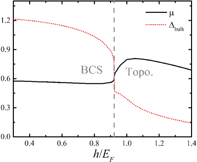
where is the Fermi-Dirac distribution function at a temperature . It is important to note that the use of Nambu spinor representation doubles the size of Hilbert space of the system. As a result, there is a particle-hole symmetry in the Bogoliubov solutions: for any “particle” solution with the wave function and energy , we can always find the other “hole” solution with a wave function and energy . Generally these two states describe the same physical state. To remove this redundancy, we have added an extra factor of in the expressions for the order parameter (6) and total density (7). In the following discussions, we focus at zero temperature with a typical interaction strength , the SOC strength . As shown in Fig. 1, the system undergoes a phase transition from a BCS superfluid to a topological superfluid when continuously increasing the effective Zeeman field over a critical value Kong et al. (2021), where the chemical potential and the bulk order parameter present a jump change. We need to emphasize that the value of will be slightly influenced by some parameters in the numerical calculation such as the size of box and the energy cutoff.
In a uniform and infinite system, the continuous momentum is a good quantum number. Thus, it is possible to get an analytic expression of four quasi-particle eigenenergy in Eq. (4) with Wei and Mueller (2012)
| (8) |
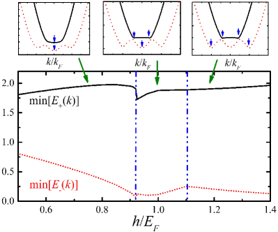
where and . The excitation of the Higgs oscillation is closely related to the minimum of quasi-particle energy Volkov and Kogan (1974). In Fig. 2, we present the positions and values of the minimum in two positive quasi-particle energy branches as a function of the Zeeman field . Typically there are three regimes separated by and , where the locations of minimum in two energy branches marked by blue arrows in three upper panels are different. The locations of minimum are both at when , then the minimum of is shifted to a nonzero momentum while the one in is still at when , and finally both of them are shifted to a nonzero momentum when .
III RESULTS AND DISCUSSION
In this work, a 1D SOC Fermi superfluid is taken into account where the quasi-1D geometry is usually realized by applying a strong confinement along both and axes in a three-dimensional (3D) system Cazalilla et al. (2011); Guan et al. (2013). In general, the order parameter is determined by the realistic parameters of the system, such as the interaction strength , the SOC strength and the effective Zeeman field . The interaction strength can be well controlled by both confinement and Feshbach resonances as discussed in references Olshanii (1998); Haller et al. (2009, 2010); Peng et al. (2010, 2011, 2014). However, it is tough to change the interaction strength rapidly or in a very short time scale. In addition, the SOC strength can not be tuned over a large range in ultracold atoms experiments. Thus, we choose the effective Zeeman field as the ramping parameter in this work. First, the Zeeman field determines directly the topological structure of the ground state as shown in Fig. 1 and we can discuss for different cases. Besides, the effective Zeeman field can be feasibly tuned in a long or short time scale by the laser intensity or the detuning in the experiments of the SOC Fermi gases. These experiment features have been introduced in Refs. Lin et al. (2011); Wang et al. (2012); Cheuk et al. (2012); Zhang et al. (2012); Williams et al. (2013); Qu et al. (2013). In order to excite and investigate the Higgs oscillation, we begin with an initial Zeeman field to calculate self-consistently its ground state, and then vary over time in a slow linear ramp way or by abruptly changing to reach a final Zeeman field . Therefore, the dynamics of the order parameter can be then studied by solving the time-dependent BdG equation
| (9) |
III.1 Slow ramp of the effective Zeeman field
We begin with a slow linear ramp of the Zeeman field , namely , in which is the time consumed to arrive at the final Zeeman field . Generally the order of can not be very small to make the system evolve in an almost adiabatic process. So should be at least in an order of .
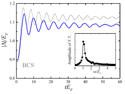
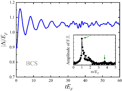
We first choose an initial Zeeman field , and linearly decrease to in a time regime . Obviously , which means that the system is in the BCS state. As shown by a smooth blue solid line in Fig. 3, the amplitude of the order parameter first increases monotonically from (i.e., the equilibrium value of at obtained from Eq. (4)), and then oscillates around an average value (i.e., almost the equilibrium value of at ). The oscillation period can be determined by the Fourier analysis of the oscillation of the order parameter. As shown in the inset, there’s a frequency peak at in the Fourier analysis, giving rise to an oscillation period at about . In addition, Volkov and Kogan predicted that the oscillation period of the Higgs oscillation should be Volkov and Kogan (1974)
| (10) |
where is usually the minimum of quasi-particle energy, and here
| (11) |
is equal to a half of the minimum energy to break a Cooper pair. Here the chemical potential and the Zeeman field in Eq. (8) should use their values at the final state (), while the order parameter should take the value of Scott et al. (2012). And we find , which is quite close to the numerical value obtained from the Fourier analysis with a deviation rate about . For comparison, we also simulate with another set of parameters (i.e., from to denoted by gray dotted line), and the difference rate between and the numerically calculated one is also around . So the Higgs oscillation here is closely related to the excitation in the lower branch of quasi-particle spectrum, and we call it the low Higgs oscillation in the following discussion.
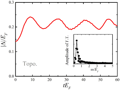
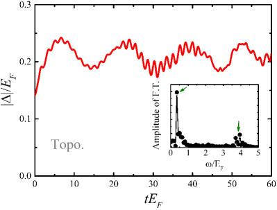
We now turn to consider the topological superfluid where both values of the initial and final Zeeman field are larger than the critical one . The Zeeman field is linearly tuned from to . We can know from Fig. 1 that increasing the Zeeman field in the topological state will generally decreases the corresponding order parameter in equilibrium. In Fig. 4, we find a similar oscillation in the amplitude of the order parameter as in the case of the BCS superfluid, around an almost equilibrium value . Similarly, we can figure out the oscillation period from the Fourier analysis, which also agrees well with the theoretical prediction within a deviation. Obviously this is also a low Higgs oscillation, originated from the excitation in the lower quasi-particle spectrum . It should also be noted that there are some tiny sawtooth-like structures in the oscillation curve at relatively large time, which make the curve not so smooth. In fact these detailed structures are closely associated to the other Higgs oscillation which will be discussed in the next subsection.
Overall, we find that the oscillation period of the Higgs oscillation obtained numerically from its dynamics agrees well with Volkov and Kogan’s prediction in both the BCS superfluid and the topological one. Moreover, we also run simulation and make the Zeeman field come into the regime , and investigate the Higgs oscillation there. However, we find a complex oscillating behaviour in the order parameter, and the numerical result of the period is quite far away from due to the rapid variation of and (see Fig. 1), or the switch of the position of minimum in the spectrum (see Fig. 2). Here we argue that these two reasons make Volkov and Kogan’s prediction can not work well in this regime.
III.2 Abrupt ramp of the effective Zeeman field
In this subsection, we consider an abrupt way to vary the Zeeman field, and investigate the following quench dynamics of the system. Similarly we prepare the system in the ground state at an initial Zeeman field , and then change immediately the Zeeman field to its destination value at time .
We first discuss the case in the topological superfluid by suddenly tuning the Zeeman field from to and study the quench dynamics of the system. The result of the oscillating behaviour in the order parameter and the associated Fourier analysis are present in Fig. 5. In contrast to the single oscillation period in the conventional 3D Fermi gas Scott et al. (2012), we find that there exist two distinct periods in the amplitude of the order parameter oscillating around . is usually smaller than the equilibrium value of the order parameter at in the case of an abrupt ramp. The bigger period originates from the excitation in the lower branch of the energy spectrum, as we discussed in the last subsection and in Fig. 4. However, we find that the smaller period, i.e., the sawtooth-like structure in the oscillation, can be well explained by the excitation to the higher branch in Eq. (8) in the quasi-particle energy spectrum, giving rise to the other excitation gap energy
| (12) |
for calculating the theoretical value using Volkov and Kogan’s prediction Volkov and Kogan (1974). The existence of two types of the Higgs oscillation can be also seen clearly from the Fourier analysis in the inset of Fig. 5 which presents two frequency peaks at and marked by two arrows. The low-frequency peak represents the low Higgs oscillation coming from the lower energy branch , while the high-frequency peak supports the other Higgs oscillation with a smaller period . This Higgs oscillation with a small period can be called the high Higgs oscillation, and has an about deviation from Volkov and Kogan’s prediction using the higher branch in the quasi-particle spectrum. Here, the ratio between two periods is about , sufficiently large to make these two Higgs oscillations can be clearly distinguished.
Likewise, we then turn to consider the existence of high Higgs oscillation in the quench dynamics of the BCS state, which has not been probed in the case of a slow ramp as in Fig. 3. We illustrate the results in Fig. 6 by preparing a ground state at and then suddenly changing the Zeeman field to at time . In general, the order parameter oscillates around , and displays an almost clear period for . However, a complex oscillation behaviour turns out at larger time, and makes it very tough to distinguish the periodic oscillation by naked eyes. Similarly, by means of the Fourier analysis of the oscillation dynamics, we can also find two frequency peaks marked by two arrows in the inset of Fig. 6. Using the peak frequency, the calculated periods of these two periodic oscillations are and respectively, which just fit well with Volkov and Kogan’s prediction and using two energy branches in the quasi-particle spectrum. Compared with the topological case in Fig. 5, the low-frequency peak of the low Higgs oscillation here is still remarkable, while the signal of the high Higgs oscillation is relatively much weaker. In fact similar to other resonance phenomena, these two Higgs oscillations are always coupled with each other, only a large period (or frequency) contrast can help to distinguish them. However, the period ratio here is much smaller than the one in the topological case, which is consistent with the expectation from Fig. 2, i.e., the minima of two energy branches approaching each other. Thus, these factors make two Higgs oscillations tangled with each other and display a complex dynamical behaviour in Fig. 6.
III.3 Further verification of two Higgs oscillations
To further probe and study these two Higgs oscillations in both the BCS and topological states, we introduce a new way to tune the Zeeman field following the resonance theory. In the last two sections, we find that the Volkov and Kogan’s prediction and agree well with the corresponding numerical results. Thus, we can use these frequencies calculated theoretically as a driving frequency to excite two Higgs oscillations respectively in only oscillation periods (longer driving-resonance time can do help to strengthen the resonance effect and is beneficial to the associated Fourier analysis), and stop driving in the following time, namely
| (13) |
with being a small amplitude of the perturbation. In fact a larger value of will not only strengthen the amplitude of oscillation, but also possibly make the system comes into different regimes as shown in Fig. 2. So we choose in the following discussions. With this periodic ramp strategy described above, we can then investigate its evolving dynamics at an initial Zeeman field .
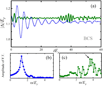
In the BCS state with a Zeeman field , we find two different oscillations in the amplitude of the order parameter as anticipated. The behaviour is shown in Fig. 7 (a), where the blue dotted line depicts the low Higgs oscillation with a big oscillation period, and the olive solid line is the high Higgs oscillation with a much smaller period. The big period contrast of these two Higgs oscillations makes it quite easy to distinguish each other by naked eyes. In panels (b) and (c) of Fig. 7, the corresponding results from the Fourier analysis are present and agree well with Volkov and Kogan’s prediction in Eq. (10). The low Higgs oscillation in the blue solid line on the left panel exhibits a clear low-frequency peak at (i.e., ), not far from the position of the high-frequency peak for the high Higgs oscillation marked by an arrow on the right panel. The lower peaks in (c) are from coupling effect of the Higgs oscillation to other excitations, and we have checked that this coupling can be weakened by taking a relatively larger driving amplitude .
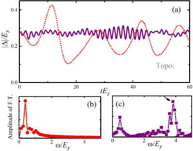
In addition, we show the results in the topological phase in Fig. 8 with where two Higgs oscillations are manifested in two significant oscillating behaviours of the order parameter. Different with the case in the BCS state, it is now much easier to distinguish two Higgs oscillations owing to their larger period contrast which may weaken the coupling between two Higgs oscillations following the resonance theory. The Fourier analysis in panels (b) and (c) of Fig. 8 further verifies the existence of two Higgs oscillations and shows an excellent agreement with the Volkov and Kogan’s prediction in Eq. (10).
In a word from Figs. 7 and 8, we can clearly distinguish the high Higgs oscillation (solid lines) and the low Higgs oscillation (dotted lines) by this periodic ramp strategy in Eq. (13) using their own driving frequency calculated from Volkov and Kogan’s prediction at fixed periods. The oscillation amplitude of low Higgs oscillation is always larger than that of the high Higgs oscillation in both the BCS superfluid and the topological superfluid. We use this strategy to further verify the existence of two Higgs oscillations which can be determined by two energy branches in the quasi-particle spectrum. The large period contrast in the topological state makes it much easier to display these two Higgs oscillations than that in the BCS state.
IV CONCLUSIONS
In summary, we theoretically probe and study two Higgs oscillations in a one-dimensional Raman-type spin-orbit-coupled Fermi superfluid, by solving the time-dependent BdG equations with three different ways to tune the effective Zeeman field. In contrast to the single Higgs oscillation in the conventional Fermi superfluid, we find two distinct Higgs oscillations in both the BCS and topological states when investigating numerically the oscillation of the order parameter. The Higgs oscillation can be well explained from the excitation in two quasi-particle energy spectrum, whose oscillation periods exhibit a great agreement with previous Volkov and Kogan’s theoretical prediction over a large range of the Zeeman field except for crossing the phase transition point. Further research could be undertaken to thoroughly explore the oscillation behaviours related to other physical observables, such as density and spin polarization.
Acknowledgements.
We are grateful for fruitful discussions with Shi-Guo Peng and kind help from Huaisong Zhao. This research was supported by the National Natural Science Foundation of China, Grants No. 11804177 (P.Z.), the Science Foundation of Zhejiang Sci-Tech University (ZSTU) No. 21062339-Y and China Postdoctoral Science Foundation No. 2020M680495 (X.L.C.).References
- Littlewood and Varma (1981) P. B. Littlewood and C. M. Varma, “Gauge-invariant theory of the dynamical interaction of charge density waves and superconductivity,” Phys. Rev. Lett. 47, 811–814 (1981).
- Littlewood and Varma (1982) P. B. Littlewood and C. M. Varma, “Amplitude collective modes in superconductors and their coupling to charge-density waves,” Phys. Rev. B 26, 4883–4893 (1982).
- Sooryakumar and Klein (1980) R. Sooryakumar and M. V. Klein, “Raman scattering by superconducting-gap excitations and their coupling to charge-density waves,” Phys. Rev. Lett. 45, 660–662 (1980).
- Sooryakumar and Klein (1981) R. Sooryakumar and M. V. Klein, “Raman scattering from superconducting gap excitations in the presence of a magnetic field,” Phys. Rev. B 23, 3213–3221 (1981).
- Matsumoto et al. (2004) Masashige Matsumoto, B. Normand, T. M. Rice, and Manfred Sigrist, “Field- and pressure-induced magnetic quantum phase transitions in ,” Phys. Rev. B 69, 054423 (2004).
- Rüegg et al. (2008) Ch. Rüegg, B. Normand, M. Matsumoto, A. Furrer, D. F. McMorrow, K. W. Krämer, H. U. Güdel, S. N. Gvasaliya, H. Mutka, and M. Boehm, “Quantum magnets under pressure: Controlling elementary excitations in ,” Phys. Rev. Lett. 100, 205701 (2008).
- Scott et al. (2012) R. G. Scott, F. Dalfovo, L. P. Pitaevskii, and S. Stringari, “Rapid ramps across the bec-bcs crossover: A route to measuring the superfluid gap,” Phys. Rev. A 86, 053604 (2012).
- Altman and Auerbach (2002) Ehud Altman and Assa Auerbach, “Oscillating superfluidity of bosons in optical lattices,” Phys. Rev. Lett. 89, 250404 (2002).
- Pollet and Prokof’ev (2012) L. Pollet and N. Prokof’ev, “Higgs mode in a two-dimensional superfluid,” Phys. Rev. Lett. 109, 010401 (2012).
- Bissbort et al. (2011) Ulf Bissbort, Sören Götze, Yongqiang Li, Jannes Heinze, Jasper S. Krauser, Malte Weinberg, Christoph Becker, Klaus Sengstock, and Walter Hofstetter, “Detecting the amplitude mode of strongly interacting lattice bosons by bragg scattering,” Phys. Rev. Lett. 106, 205303 (2011).
- Endres et al. (2012) Manuel Endres, Takeshi Fukuhara, David Pekker, Marc Cheneau, Peter Schau, Christian Gross, Eugene Demler, Stefan Kuhr, and Immanuel Bloch, “The ‘higgs’ amplitude mode at the two-dimensional superfluid/mott insulator transition,” Nature 487, 454–458 (2012).
- Pekker and Varma (2015) David Pekker and C.M. Varma, “Amplitude/higgs modes in condensed matter physics,” Annual Review of Condensed Matter Physics 6, 269–297 (2015).
- Matsunaga et al. (2013) Ryusuke Matsunaga, Yuki I. Hamada, Kazumasa Makise, Yoshinori Uzawa, Hirotaka Terai, Zhen Wang, and Ryo Shimano, “Higgs amplitude mode in the bcs superconductors induced by terahertz pulse excitation,” Phys. Rev. Lett. 111, 057002 (2013).
- Sherman et al. (2015) Daniel Sherman, Uwe S Pracht, Boris Gorshunov, Shachaf Poran, John Jesudasan, Madhavi Chand, Pratap Raychaudhuri, Mason Swanson, Nandini Trivedi, Assa Auerbach, et al., “The higgs mode in disordered superconductors close to a quantum phase transition,” Nature Physics 11, 188–192 (2015).
- Yuzbashyan and Dzero (2006) Emil A. Yuzbashyan and Maxim Dzero, “Dynamical vanishing of the order parameter in a fermionic condensate,” Phys. Rev. Lett. 96, 230404 (2006).
- Hannibal et al. (2015) S. Hannibal, P. Kettmann, M. D. Croitoru, A. Vagov, V. M. Axt, and T. Kuhn, “Quench dynamics of an ultracold fermi gas in the bcs regime: Spectral properties and confinement-induced breakdown of the higgs mode,” Phys. Rev. A 91, 043630 (2015).
- Altman and Vishwanath (2005) Ehud Altman and Ashvin Vishwanath, “Dynamic projection on feshbach molecules: A probe of pairing and phase fluctuations,” Phys. Rev. Lett. 95, 110404 (2005).
- Perali et al. (2005) A. Perali, P. Pieri, and G. C. Strinati, “Extracting the condensate density from projection experiments with fermi gases,” Phys. Rev. Lett. 95, 010407 (2005).
- Matyjaśkiewicz et al. (2008) S. Matyjaśkiewicz, M. H. Szymańska, and K. Góral, “Probing fermionic condensates by fast-sweep projection onto feshbach molecules,” Phys. Rev. Lett. 101, 150410 (2008).
- Behrle et al. (2018) A Behrle, T Harrison, J Kombe, K Gao, M Link, J-S Bernier, C Kollath, and M Köhl, “Higgs mode in a strongly interacting fermionic superfluid,” Nature Physics 14, 781–785 (2018).
- Liu et al. (2016) Boyang Liu, Hui Zhai, and Shizhong Zhang, “Evolution of the higgs mode in a fermion superfluid with tunable interactions,” Phys. Rev. A 93, 033641 (2016).
- Han et al. (2016) Xinloong Han, Boyang Liu, and Jiangping Hu, “Observability of higgs mode in a system without lorentz invariance,” Phys. Rev. A 94, 033608 (2016).
- Kurkjian et al. (2019) H. Kurkjian, S. N. Klimin, J. Tempere, and Y. Castin, “Pair-breaking collective branch in bcs superconductors and superfluid fermi gases,” Phys. Rev. Lett. 122, 093403 (2019).
- Volkov and Kogan (1974) AF Volkov and Sh M Kogan, “Collisionless relaxation of the energy gap in superconductors,” Soviet Journal of Experimental and Theoretical Physics 38, 1018 (1974).
- Wang et al. (2012) Pengjun Wang, Zeng-Qiang Yu, Zhengkun Fu, Jiao Miao, Lianghui Huang, Shijie Chai, Hui Zhai, and Jing Zhang, “Spin-orbit coupled degenerate fermi gases,” Phys. Rev. Lett. 109, 095301 (2012).
- Cheuk et al. (2012) Lawrence W. Cheuk, Ariel T. Sommer, Zoran Hadzibabic, Tarik Yefsah, Waseem S. Bakr, and Martin W. Zwierlein, “Spin-injection spectroscopy of a spin-orbit coupled fermi gas,” Phys. Rev. Lett. 109, 095302 (2012).
- Wang et al. (2015) Pei Wang, Wei Yi, and Gao Xianlong, “Topological phase transition in the quench dynamics of a one-dimensional fermi gas with spin–orbit coupling,” New Journal of Physics 17, 013029 (2015).
- Dong et al. (2015) Ying Dong, Lin Dong, Ming Gong, and Han Pu, “Dynamical phases in quenched spin–orbit-coupled degenerate fermi gas,” Nature Communications 6, 6103 (2015).
- Kong et al. (2021) Lingchii Kong, Genwang Fan, Shi-Guo Peng, Xiao-Long Chen, Huaisong Zhao, and Peng Zou, “Dynamical generation of solitons in one-dimensional fermi superfluids with and without spin-orbit coupling,” Phys. Rev. A 103, 063318 (2021).
- Wei and Mueller (2012) Ran Wei and Erich J. Mueller, “Majorana fermions in one-dimensional spin-orbit-coupled fermi gases,” Phys. Rev. A 86, 063604 (2012).
- Cazalilla et al. (2011) M. A. Cazalilla, R. Citro, T. Giamarchi, E. Orignac, and M. Rigol, “One dimensional bosons: From condensed matter systems to ultracold gases,” Rev. Mod. Phys. 83, 1405–1466 (2011).
- Guan et al. (2013) Xi-Wen Guan, Murray T. Batchelor, and Chaohong Lee, “Fermi gases in one dimension: From bethe ansatz to experiments,” Rev. Mod. Phys. 85, 1633–1691 (2013).
- Olshanii (1998) M. Olshanii, “Atomic scattering in the presence of an external confinement and a gas of impenetrable bosons,” Phys. Rev. Lett. 81, 938–941 (1998).
- Haller et al. (2009) Elmar Haller, Mattias Gustavsson, Manfred J. Mark, Johann G. Danzl, Russell Hart, Guido Pupillo, and Hanns-Christoph Nägerl, “Realization of an excited, strongly correlated quantum gas phase,” Science 325, 1224–1227 (2009), https://www.science.org/doi/pdf/10.1126/science.1175850 .
- Haller et al. (2010) Elmar Haller, Manfred J. Mark, Russell Hart, Johann G. Danzl, Lukas Reichsöllner, Vladimir Melezhik, Peter Schmelcher, and Hanns-Christoph Nägerl, “Confinement-induced resonances in low-dimensional quantum systems,” Phys. Rev. Lett. 104, 153203 (2010).
- Peng et al. (2010) Shi-Guo Peng, Seyyed S. Bohloul, Xia-Ji Liu, Hui Hu, and Peter D. Drummond, “Confinement-induced resonance in quasi-one-dimensional systems under transversely anisotropic confinement,” Phys. Rev. A 82, 063633 (2010).
- Peng et al. (2011) Shi-Guo Peng, Hui Hu, Xia-Ji Liu, and Peter D. Drummond, “Confinement-induced resonances in anharmonic waveguides,” Phys. Rev. A 84, 043619 (2011).
- Peng et al. (2014) Shi-Guo Peng, Shina Tan, and Kaijun Jiang, “Manipulation of -wave scattering of cold atoms in low dimensions using the magnetic field vector,” Phys. Rev. Lett. 112, 250401 (2014).
- Lin et al. (2011) Y.-J. Lin, K. Jiménez-García, and I. B. Spielman, “Spin–orbit-coupled bose–einstein condensates,” Nature 471, 83–86 (2011).
- Zhang et al. (2012) Jin-Yi Zhang, Si-Cong Ji, Zhu Chen, Long Zhang, Zhi-Dong Du, Bo Yan, Ge-Sheng Pan, Bo Zhao, You-Jin Deng, Hui Zhai, Shuai Chen, and Jian-Wei Pan, “Collective dipole oscillations of a spin-orbit coupled bose-einstein condensate,” Phys. Rev. Lett. 109, 115301 (2012).
- Williams et al. (2013) R. A. Williams, M. C. Beeler, L. J. LeBlanc, K. Jiménez-García, and I. B. Spielman, “Raman-induced interactions in a single-component fermi gas near an -wave feshbach resonance,” Phys. Rev. Lett. 111, 095301 (2013).
- Qu et al. (2013) Chunlei Qu, Chris Hamner, Ming Gong, Chuanwei Zhang, and Peter Engels, “Observation of zitterbewegung in a spin-orbit-coupled bose-einstein condensate,” Phys. Rev. A 88, 021604 (2013).