Present address: ]Department of Engineering Science, The University of Electro-Communications, Chofu 182-8585, Japan
Probing exciton dynamics with spectral selectivity through the use of quantum entangled photons
Abstract
Quantum light is increasingly recognized as a promising resource for developing optical measurement techniques. Particular attention has been paid to enhancing the precision of the measurements beyond classical techniques by using nonclassical correlations between quantum entangled photons. Recent advances in quantum optics technology have made it possible to manipulate the spectral and temporal properties of entangled photons, and the photon correlations can facilitate the extraction of matter information with relatively simple optical systems compared to conventional schemes. In these respects, the applications of entangled photons to time-resolved spectroscopy can open new avenues for unambiguously extracting information on dynamical processes in complex molecular and materials systems. Here, we propose time-resolved spectroscopy in which specific signal contributions are selectively enhanced by harnessing the nonclassical correlations of entangled photons. The entanglement time characterizes the mutual delay between an entangled twin and determines the spectral distribution of the photon correlations. The entanglement time plays a dual role as the knob for controlling the accessible time region of dynamical processes and the degrees of spectral selectivity. In this sense, the role of the entanglement time is substantially equivalent to the temporal width of the classical laser pulse. The results demonstrate that the application of quantum entangled photons to time-resolved spectroscopy leads to monitoring dynamical processes in complex molecular and materials systems by selectively extracting desired signal contributions from congested spectra. We anticipate that more elaborately engineered photon states would broaden the availability of quantum light spectroscopy.
I Introduction
In recent years, quantum light has been recognized as an important resource for the development of quantum metrology, where nonclassical features of light are exploited to enhance the precision and resolution of optical measurements beyond classical techniques Pirandola et al. (2018); Moreau et al. (2019). One of the striking features of quantum light is quantum entanglement. It is a phenomenon where the state of an entire system cannot be described as the product of the quantum states of its individual constituent particles. For instance, the use of photon entanglement has enabled ghost imaging Pittman et al. (1995), quantum imaging with undetected photons Lemos et al. (2014), quantum lithography Boto et al. (2000), cancellation of even-order dispersion Franson (1992), quantum optical coherence tomography Abouraddy et al. (2002); Nasr et al. (2003); Okano et al. (2015), and realization of sub-shot-noise microscopy Ono, Okamoto, and Takeuchi (2013); Triginer Garces et al. (2020); Casacio et al. (2021).
With recent advances in quantum optical technologies, entangled photons have become a promising avenue for the development of new spectroscopic techniques Gea-Banacloche (1989); Javanainen and Gould (1990); Saleh et al. (1998); Oka (2010); Schlawin and Mukamel (2013); de J León-Montiel et al. (2019); Fujihashi, Shimizu, and Ishizaki (2020); Debnath and Rubio (2020); Szoke et al. (2020); Mukamel et al. (2020); Muñoz, Frascella, and Schlawin (2021); Raymer, Landes, and Marcus (2021); Chen and Mukamel (2021); Dorfman et al. (2021); Asban, Dorfman, and Mukamel (2021); Asban and Mukamel (2021); Asban, Chernyak, and Mukamel (2022); Chen and Mukamel (2022); Albarelli et al. (2023); Li et al. (2023). It was experimentally demonstrated that nonclassical correlations between entangled photons had several advantages in spectroscopy, including sub-shot-noise absorption spectroscopy Tapster, Seward, and Rarity (1991); Brida, Genovese, and Berchera (2010); Matsuzaki and Tahara (2022) and increased two-photon absorption signal intensity Georgiades et al. (1995); Dayan et al. (2004); Lee and Goodson, III (2006); Upton et al. (2013); Varnavski and Goodson III (2020). Entanglement-induced two-photon transparency Fei et al. (1997) and suppression of exciton transport Schlawin et al. (2013) controlling the entanglement time, which is the hallmark of the non-classical photon correlation, were also theoretically investigated. In addition to the above advantages, the nonclassical correlations can be used to obtain spectroscopic signals with simpler optical systems compared with conventional methods Yabushita and Kobayashi (2004); Kalashnikov et al. (2016); Mukai et al. (2021); Arahata et al. (2022); Kalashnikov et al. (2017); Eshun et al. (2021). For example, infrared spectroscopy with visible-light source and detector was performed by exploiting entangled visible and infrared photons generated via parametric down-conversion (PDC) Kalashnikov et al. (2016); Mukai et al. (2021); Arahata et al. (2022). Furthermore, the Hong–Ou–Mandel interferometer with entangled photons allows the measurement of the dephasing time of molecules at the femtosecond time scale without the need for ultrashort laser pulses Kalashnikov et al. (2017); Eshun et al. (2021). Inspired by the capabilities of such nonclassical photon correlations, the applications to time-resolved spectroscopic measurements have been theoretically discussed Dorfman, Schlawin, and Mukamel (2014); Schlawin, Dorfman, and Mukamel (2016); Zhang et al. (2022); Fan, Ou, and Zhang (2023). The development of time-resolved spectroscopy that enhances the precision and resolution beyond classical techniques may lead to a better understanding of the mechanism of dynamical processes in complex molecules, such as photosynthetic light-harvesting systems. In contrast to many experimental and theoretical studies on entangled two-photon absorption, only a few theoretical studies have reported the application of entangled photons to time-resolved spectroscopic measurements. There is no comprehensive understanding of which nonclassical states of light are suitable for implementing real-time observation of dynamical processes in condensed phases and which nonclassical photon correlations allow the manipulation of nonlinear signals in a way that cannot be achieved with classical pulses.
In a previous study, we developed a theory of frequency-dispersed transmission measurement using entangled photon pairs generated via PDC pumped with a monochromatic laser Ishizaki (2020a). Especially, it was demonstrated that this measurement scheme enabled time-resolved spectroscopy based on monochromatic pumping when the entanglement time is sufficiently short. Chen et al. demonstrated that a similar scheme could be applied to monitor ultrafast electronic-nuclear motion at conical intersection Chen, Gu, and Mukamel (2022); Gu et al. (2023). Moreover, the simple model calculations in Refs. 53 and 56 suggested that for a finite value of entanglement time, the spectral distribution of the phase-matching function works as a sinc filter in signal processing Owen (2007), which can be used to selectively resolve a specific region of the spectra. Therefore, this spectral filtering mechanism is expected to simplify the interpretation of the spectra in complex molecules.
In this study, we theoretically propose a time-resolved spectroscopy scheme that selectively enhances specific signal contributions by harnessing the nonclassical correlations between entangled photons. We apply our spectroscopic scheme to a photosynthetic pigment-protein complex, and demonstrated that the phase-matching functions of the PDC in nonlinear crystals, such as periodically poled crystal and - crystal, allow one to separately measure specific peaks of spectra by tuning the entanglement time and the central frequencies of the entangled photons. Furthermore, we investigated whether the spectral filtering mechanism could be implemented in the range of currently available entangled photon sources.
II Theory
According to the phase matching conditions, the PDC process can be triggered in different geometries: One distinguishes type-I and type-II, and type-0 down-conversion. For simplicity, we consider a type-II PDC in a birefringent crystal Mandel and Wolf (1995) because the wave vector mismatch can be well approximated to linear order in frequency Grice and Walmsley (1997); Keller and Rubin (1997), as described in Eq. (3). The intensity and normalized spectral envelope of the pump laser are denoted as and , respectively. A photon of frequency in the pump laser is split into a pair of entangled photons whose frequencies and must satisfy because of energy conservation. The polarizations of the generated twins are orthogonal to each other and characterized by horizontal (H) and vertical (V) polarizations. In the weak-down conversion regime, the quantum state of the twin is expressed as Grice and Walmsley (1997); Keller and Rubin (1997)
| (1) |
where the operator creates a photon of frequency and polarization and the function is the two-photon amplitude. For simplicity, in Eq. (1), we neglected the spatial variation of the two-photon amplitude and the spatial propagation direction is selected by the collinear configuration Schlawin, Dorfman, and Mukamel (2018). In the following, we consider the electric fields inside a one-dimensional (1D) nonlinear crystal of length . Thus, the two-photon amplitude is given by , where is the normalized pump envelope and the sinc function originates from phase-matching Boyd (2003); Graffitti et al. (2018). Note that here is not necessarily normalized, as . Expanding the wave vector mismatch to first order in the frequencies and around the center frequencies of the generated beams, and , we obtain with , where and are the group velocities of the pump laser and one of the generated beams at central frequency , respectively Keller and Rubin (1997); Rubin et al. (1994). The central frequencies and group velocities are evaluated using the Sellmeier equations Dmitriev, Gurzadyan, and Nikogosyan (2013), which provide empirical relations between the refractive indices of the crystals and the frequencies of the generated beams. In this study, we address the case of monochromatic pumping . Thus, the two-photon amplitude is recast as
| (2) | |||
| (3) |
The so-called entanglement time is the maximum time difference between twin photons leaving the crystal Saleh et al. (1998). The positive frequency component of the field operator is given by: where and the negative frequency component is . The unit vectors and indicate the directions of the horizontal and vertical polarizations, respectively. We adopt the slowly varying envelope approximation, in which the bandwidth of the field is assumed to be negligibly narrow in comparison with the central frequency Mandel and Wolf (1995). This approximation allows treating the factor as a constant . All other constants are merged into a factor , which is regarded as the conversion efficiency of the PDC.
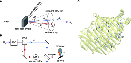
We consider the setup shown in Fig. 1. Twin photons were split using a polarized beam splitter. Although the relative delay between horizontally and vertically polarized photons is innately determined by the entanglement time, the delay interval is further controlled by adjusting the path difference between the beams Hong, Ou, and Mandel (1987); Franson (1989). This controllable delay is denoted by in this study. Direct observation of time-frequency duality of biphotons over a delay time of at least a few picoseconds has been experimentally demonstrated Jin, Saito, and Shimizu (2018); MacLean, Donohue, and Resch (2018). The field operator is expressed as , indicating that the horizontally and vertically polarized photons act as the pump and probe field for the molecules, respectively. The probe field transmitted through the sample is frequency-dispersed, and the change in the transmitted photon number is registered as a function of the frequency , pump frequency , and external delay , yielding the signal .
The Hamiltonian used to describe this pump–probe process is written as . The first term gives the Hamiltonian of the photoactive degrees of freedom (DOFs) in molecules. The second term describes the free electric field. In this work, the electronic ground state , single-excitation manifold , and double-excitation manifold are considered as photoactive DOFs. The overline of the subscripts indicates the state in the double-excitation manifold. The optical transitions are described by the dipole operator , where and . The rotating-wave approximation enables the expression of the molecule-field interaction as . The signal is expressed as Dorfman, Schlawin, and Mukamel (2016)
| (4) |
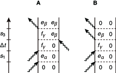
where and . We expand the density operator with respect to to the third order, resulting in the sum of eight contributions classified as stimulated emission (SE), ground-state bleaching (GSB), excited-state absorption (ESA), and double quantum coherence (DQC). The DQC signal decays rapidly in comparison with the others when is sufficiently long compared to the timescale of environmental reorganization (see Section S1 of Supplementary Material for details); hence, the DQC is disregarded in this work. Each contribution is expressed as follows:
| (5) |
where indicates rephasing (r) or non-rephasing (nr), and indicates the GSB, SE, or ESA. Here, and are the third-order response functions of the molecules and four-body correlation functions of the field operators, respectively.
For demonstration purposes, we focused on rephasing the SE contribution. Details of the GSB and ESA are provided in Section S2 of Supplementary Material. The rephasing SE contribution is given by . Here, we have defined , where the brackets represent the average over molecular orientations Schlau-Cohen, Ishizaki, and Fleming (2011); Schlawin (2022). The matrix element of the time-evolution operator is defined by , and is the abbreviation of . By substituting the response function and field correlation function Ishizaki (2020a) into Eq. (5), we obtain the following SE signal:
| (6) |
where . The second term in Eq. (6) originates from a field commutator. This term does not depend on . Therefore, the contribution to the signal can be ignored by considering the difference spectrum:
| (7) |
The Fourier–Laplace transform of is written as , and is defined as
| (8) |
where . As discussed in Ref. 53, Eq. (8) for can be simplified as
| (9) |
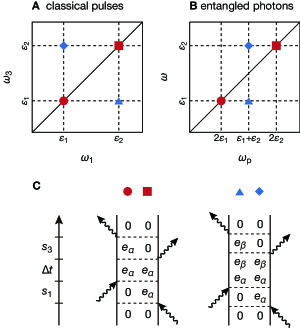
which is independent of . To obtain the information contents of the signal, we assume that the time evolution in the and periods is described as , thereby leading to the expression of the rephasing SE signal, . It can be understood that the non-classical correlation between the entangled photon pair generated via the PDC pumped with a monochromatic laser restricts the possible optical transitions, (, ), for a given pump frequency. Therefore, Eqs. (6) and (9) indicate that the state-to-state dynamics in the molecules are temporally resolved by sweeping the external delay in the time region longer than half of the entanglement time, . It should be mentioned that phenomena similar to the specific selective excitation described above have been discussed in Ref. 42 in the context of manipulation of two-excitation distributions by the non-classical photon correlation.
Notably, in the limit , the third-order signal in Eq. (4) corresponds to the spectral information along the anti-diagonal line of the absorptive 2D spectrum obtained using the photon-echo technique in the impulsive limit:
| (10) |
except for the -independent term Ishizaki (2020a), as shown in Fig. 2 (the explicit expression of the 2D photon-echo spectrum, , is given in Appendix B). It is noted that the sign of the quantum spectrum, , is the opposite of the sign of the classical 2D photon-echo spectrum, , as shown in Eq. (10). In the following numerical results, the spectrum is plotted multiplied by a minus sign for clarity. Equation (10) also indicates that the pump-probe signal shows no collective two-particle contributions (see Section S3 of Supplementary Material for details). This result is consistent with the arguments in Refs. 73; 74.
Furthermore, the phase matching function in Eq. (6) can selectively enhance a specific spectral region of the signal by varying the center frequency of the generated beam. The width at half maximum of is approximately given by . Interestingly, this corresponds to a sinc filter in signal processing Owen (2007). Therefore, the entanglement time plays a dual role of the knob for controlling the accessible time region of the dynamics in molecules, , and the degree of spectral selectivity, . It is noted that similar spectral filtering can be realized with classical light O’shea et al. (2001), and has been utilized for selective excitation in multidimensional spectra Tollerud, Hall, and Davis (2014).
III Numerical results
In the following, we discuss roles of the entanglement time on the temporal resolution and spectral selectivity through numerical investigations of the signals in Eqs. (6)–(8) and Eqs. (S7)–(S11) of the Fenna-Matthews-Olson (FMO) pigment-protein complex in the photosynthetic green sulfur bacterium Chlorobium tepidum Li et al. (1997); Camara-Artigas, Blankenship, and Allen (2003); Tronrud et al. (2009) (Fig. 1C). Due to its relatively small size, it has been widely studied experimentally and theoretically as a prototypical system for discussing photosynthetic energy transfer using nonlinear optical spectroscopy Freiberg et al. (1997); Brixner et al. (2005); Engel et al. (2007); Fujihashi, Fleming, and Ishizaki (2015). Our model includes seven single-excitation states and 21 double-excitation states (for details on the model, see Appendix A). The matrix elements and in Eq. (6) and Eqs. (S7)–(S11) are calculated using the cumulant expansion for the fluctuations in the electronic energies and the modified Redfield theory Zhang et al. (1998) (see Appendix A).
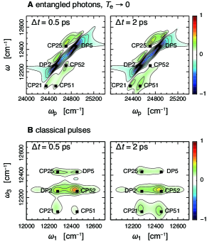
III.1 Limit of short entanglement time
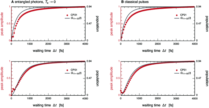
We investigate the correspondence between the classical 2D Fourier-transformed photon-echo signal and the transmission signal with entangled photons. Figure 3A presents the difference spectra, , with quantum-entangled photon pairs in the limit of . The waiting times are and . The temperature was set as . For comparison, we depict the 2D photon-echo spectra, , generated by four laser pulses in the impulsive limit in Fig. 3B. For the calculations, we chose the HHVV sequence for the polarizations of the four laser pulses so that the polarization sequence was the same as that of the entangled photon pair in the limit of short entanglement time. Figure 3B shows six separate peaks at positions marked by black squares. The diagonal peaks centered in the vicinity of are labeled as DP, whereas the cross-peaks located around are labeled as CP. As can be seen in Eq. (10) and Fig. 2, in the difference spectra, peaks corresponding to DP and CP appear near and , respectively. Thus, each of the six peaks at the positions indicated by the black square in Fig. 3A shows the spectral information of the peak at the same label position in Fig. 3B. It is noted that from the definition of the difference spectrum in Eq. (7) the decay of the SE signal at finite delay times appears as a negative signal, as presented by DP2 and DP5 in Fig. 3A.
While the cross-peaks at indicate coupled excited states, the appearance of the cross-peaks with increasing waiting time, , indicates a relaxation process from a higher exciton state to a lower exciton state. As time progressed, the appearance of CP51 can be observed in Fig. 3. This behavior reflects the relaxation process, as presented in Supporting information, Fig. S2. Similarly, the increase in the peak amplitude of CP21 during was attributed to the relaxation process. However, the Liouville pathways involving , , , and states have much smaller amplitudes than CP21 and CP51. Hence, it is difficult to extract information on the energy transfer processes involving these excitation states owing to spectral congestion.
III.2 Cases of finite entanglement times
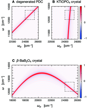
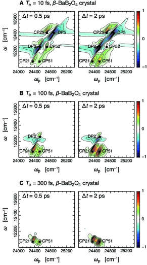
To discuss the roles of the entanglement time in the temporal resolution and spectral selectivity, we investigated cases of nondegenerate down-conversion, . A nondegenerate type-II PDC experiment in the visible frequency region is possible, for example, using a periodically poled (PPKTP) crystal Kim, Fiorentino, and Wong (2006); Fedrizzi et al. (2007) and - (BBO) crystal Yabushita and Kobayashi (2004), as shown in Fig. 4.
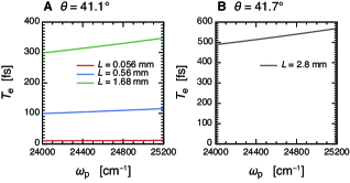
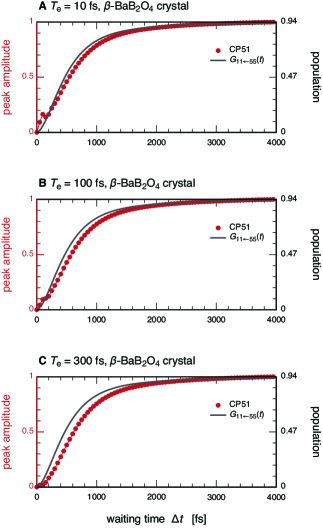
We first considered the nondegenerate PDC through the BBO crystal in the collinear configuration, where the scattering angles shown in Fig. 1A are set to . The phase-matching condition of a uniaxial birefringent crystal, such as a BBO crystal, depends on the propagation angle of the pump beam with respect to the optical axis (see Section S4 of Supplementary Material). Thus, the central frequencies of the generated twin beams can be tuned by changing the value of . Figure 5 presents the difference spectra, , as a function of and with entangled photon pairs generated via the BBO crystal for (A) , (B) , and (C) . The angle of the pump beam with respect to the optical axis is set to , where the central frequencies of the twin photons nearly resonate with the pair of optical transitions ( and ). The other parameters were the same as those shown in Fig. 3A. The value of the entanglement time in Fig. 5 was evaluated by computing the group velocities of twin photons generated when pumped at . Strictly speaking, the entanglement time depends on the value of the pump frequency because the group velocities and depend on the value of . However, the influence of this correction is small because the group velocities vary rather slowly far from the absorption resonances of the nonlinear crystal (see Supplementary Material, Fig. S1). The signal in Fig. 5A appears to be similar to that in Fig. 3A, which can be regarded as the limit for the short entanglement time. As pointed out above, the spectral distribution of the phase-matching function can selectively enhance a specific region of the spectra allowed by the bandwidth . This can be observed in Figs. 5B and C, where the intensities of the peaks except for CP21 and CP51 are suppressed with increasing entanglement time. Simultaneously, the overall behavior of the signal at CP51 in Fig. 5 is similar to the dynamics of the transport, as demonstrated in Supplementary Material, Fig. S3. It is because it is possible to extract relevant information on the excited-state dynamics from the signal in the time region longer than half of the entanglement time.
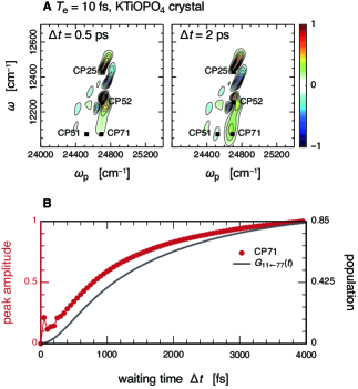
The results in Fig. 5 suggest that the spectral filter of the phase-matching function can be used to extract information on weak signal contributions masked by strong peaks. To demonstrate this ability, we investigated the case of a nondegenerate PDC using the PPKTP crystal. In the PPKTP crystal, it is possible to tune the central frequencies of the generated twin beams by changing the values of the poling period and crystal temperature (see Section S7 of Supplementary Material). Figure 6A shows the difference spectra, , as a function of and with the entangled photon pairs generated via the PPKTP crystal for . The poling period and crystal temperature were set to and , respectively, where the central frequencies of the twin photons nearly resonate with the pair of optical transitions (, ). The entanglement time was evaluated by calculating the central frequencies and group velocities of the generated twin photons when pumped at . The other parameters were the same as those shown in Fig. 3A. Figure 6B also shows the time evolution of the CP71 amplitude ( and ), as shown in Fig. 6A. For comparison, the black line shown in Fig. 6B represents the matrix element of the time-evolution operator, , which is calculated directly in the modified Redfield theory and corresponds to transport. The intensities of CP21 and CP51 shown in Fig. 6A are suppressed because of the narrow spectral filter of the phase-matching function. Consequently, the signal at CP71 in Fig. 6A is not distorted by interference with nearby cross-peak components, such as CP21 and CP51, and is better resolved compared with that in Fig. 3A. Simultaneously, the overall behavior of the signal at CP71 in Fig. 6B is similar to the dynamics of transport. Therefore, Fig. 6 demonstrates that the spectral filter of the phase-matching function can be used to selectively enhance specific peaks within the congested 2D spectra of the FMO complex by controlling the entanglement time and central frequencies of the entangled photons while maintaining the ultrafast temporal resolution.
As indicated in Figs. 5 and 6, in the case of finite entanglement time, the role of the entanglement time is substantially equivalent to the temporal width of the classical laser pulse. In this sense, entangled photon pairs do not provide simultaneous improvement in temporal and frequency resolution over spectroscopy using classical laser pulses. However, it is interesting that the non-classical correlation between the twin photons enables the selective excitations of specific single-excitation states although a simple optical system and monochromatic laser are employed. This is one aspect of the usefulness of non-classical photon correlation for spectroscopic measurements. This insight encourages us to envision that employing more intricately engineered quantum states of light could expand the applicability of quantum light spectroscopy and molecular quantum metrology.
IV Discussion
In this work, we explored the roles of entanglement time for temporal resolution and spectral selectivity through numerical investigations of the entangled photon spectroscopy of FMO complexes. The frequency-dispersed transmission measurement with entangled photons considered in our study exhibits three interesting features. First, nonclassical photon correlation enables time-resolved spectroscopy with monochromatic pumping Ishizaki (2020a). The temporal width of the entangled photon pair is determined by the entanglement time, and hence can be tuned by the crystal length. For example, as illustrated in Fig. 5A, the temporal width of the entangled photon pairs generated with the BBO crystal with a thickness of was a few femtoseconds. Therefore, transmission measurement can temporally resolve the dynamic processes of molecular systems occurring at femtosecond timescales without requiring sophisticated control of the temporal delay between femtosecond laser pulses. Second, the spectral distribution of the phase-matching function can function as a frequency filter, which removes all optical transitions that fall outside the spectral width. The spectral distribution of the phase-matching function can be manipulated by changing the crystal length and phase-matching angle. Thus, specific peaks in crowded 2D spectra can be selectively enhanced or suppressed by controlling the phase-matching function, as in laser spectroscopic experiments using narrow-band pulses. As demonstrated in Fig. 5, the selective enhancement of specific peaks in the congested 2D spectrum of the FMO complex can be achieved using the phase-matching function of the PDC process in BBO crystals with crystal lengths ranging from to , which has been used experimentally Branning, Migdall, and Sergienko (2000); Dayan et al. (2004); Yabushita and Kobayashi (2004); Lee and Goodson, III (2006); Eshun et al. (2021). Therefore, spectral filtering is feasible using current quantum optical techniques for generating entangled photons. Third, the spectral distribution of the phase-matching function strongly depends on the properties of the nonlinear crystal. As shown in Figs. 5 and 6, the spectral filter effects can easily be adjusted by changing the nonlinear crystals and/or their properties. Although we considered only BBO and PPKTP crystals in this study, there is a wide range of nonlinear crystals that have been used for PDC in the near-infrared and visible regions Dmitriev, Gurzadyan, and Nikogosyan (2013). Therefore, we anticipate that transmission measurement can be applied not only to FMO complexes but also to other photosynthetic pigment-protein complexes such as the photosystem II reaction center Romero et al. (2014); Fuller et al. (2014); Fujihashi, Higashi, and Ishizaki (2018) by finding an appropriate nonlinear crystal corresponding to the spectral range of the molecular system of interest.
The feasibility of entangled two-photon spectroscopy was recently questioned by several research groups Landes et al. (2021); Parzuchowski et al. (2021). The quantitative estimates using the upper bound on the isolated-entangled-pair cross section indicate that realistic sample concentrations event rates are orders of magnitude below the detection threshold of typical photon-counting systems Raymer, Landes, and Marcus (2021). The same difficulties are expected to be faced in the case of the transmission measurement considered in our study. One solution to overcome vanishingly weak nonlinear signals is to use high-gain squeezed vacuum states Cutipa and Chekhova (2022). As demonstrated in Section S8 of Supplementary Material, at least when the entanglement time is sufficiently short compared with characteristic timescales of the dynamics under investigation, the transmission measurement is capable of temporally resolving the excitation dynamics with high-gain squeezed vacuum states. Whether the measurement can be performed under other parameter conditions such as for long entanglement times is a subject for future research.
In the present work, we did not concentrate on the exploitation of the polarization control of entangled photon pairs. Polarization-controlled measurements have been considered a beneficial technique for separating crowded 2D spectra Hochstrasser (2001); Zanni et al. (2001); Dreyer, Moran, and Mukamel (2003); Schlau-Cohen et al. (2012); Westenhoff et al. (2012). In this regard, exploiting the polarization of entangled photons has the potential to improve the resolution of quantum spectroscopy further. Moreover, hyperentanglement in frequency-time and polarization can be generated by the type-II PDC process Kwiat (1997). Further research on the use of such more elaborately controlled quantum states of light for optical spectroscopy may lead to the development of novel time-resolved spectroscopic measurements with precision and resolution beyond the limits imposed by the laws of classical physics.
Acknowledgements.
This study was supported by JSPS KAKENHI (Grant Numbers JP17H02946 and JP21H01052) and MEXT KAKENHI (Grant Number JP17H06437) in Innovative Areas “Innovations for Light-Energy Conversion,” MEXT Quantum Leap Flagship Program (Grant Numbers JPMXS0118069242 and JPMXS0120330644). Y.F. and M.H. are grateful for the financial support from MEXT KAKENHI (Grant Number JP20H05839) in Transformative Research Areas (A), “Dynamic Exciton: Emerging Science and Innovation (20A201),” and JST PRESTO (Grant Numbers JPMJPR19G8 and JPMJPR18GA). K.M. acknowledges support from JSPS KAKENHI (Grant Number JP21K14481).Appendix A Molecular system
The molecular Hamiltonian is given by Fujihashi, Fleming, and Ishizaki (2015): The first term is the electronic excitation Hamiltonian, , where is the Franck–Condon transition energy of the th pigment, is the electronic coupling between the pigments, and the excitation creation operator is introduced for the excitation vacuum such that and . We assume that the environmental DOFs can be treated as an ensemble of harmonic oscillators with , where are the dimensionless normal-mode coordinates and and are the corresponding frequencies and momenta, respectively. The last term is the electronic-environmental interaction and is expressed as , where , and denotes the coupling constant between the th pigment and the th normal mode. In the eigenstate representation, the excitation Hamiltonian can be written as , where and .
Because are normal mode coordinates, the dynamics of can be described as a Gaussian process Kubo, Toda, and Hashitsume (1985). By applying the second-order cumulant expansion to the fluctuations in the electronic energies, the third-order response function is expressed in terms of the line-broadening function, , where is expressed as in terms of the spectral density, . The third-order response function of the molecules was computed using cumulant expansion for the fluctuations in the electronic energies Zhang et al. (1998). In this study, the spectral density is modeled as , where and represent the energy and timescale of environmental reorganization, respectively Ishizaki (2020b). The time evolution of the electronic excitations during the waiting time, , was computed in the modified Redfield theory Zhang et al. (1998); Yang and Fleming (2002).
The FMO complex is a trimer made of identical subunits, each containing eight bacteriochlorophyll a (BChla) molecules Tronrud et al. (2009). Because the eighth BChl is only loosely bound, this pigment is usually lost in the majority of the FMO complexes during the isolation procedure Tronrud et al. (2009); Schmidt am Busch et al. (2011). Therefore, we did not consider the eighth BChl concentration in this study. The parameters in the molecular Hamiltonian were obtained from Refs. 81; 104. The atomic coordinates of the FMO complex were based on the X-ray crystallographic structure (PDB code:1M50) Camara-Artigas, Blankenship, and Allen (2003). The electric transition dipoles were assumed to be placed along the – axis, and the electric dipole strength of monomeric BChla is Abramavicius, Voronine, and Mukamel (2008); Voronine, Abramavicius, and Mukamel (2008). We set the reorganization energy and relaxation time to and , respectively. We modeled static disorder by adding a Gaussian disorder (the standard deviation is ) for each diagonal term in . These values were used to fit the experimental absorption and circular dichroism spectra of the FMO complex at Abramavicius, Voronine, and Mukamel (2008); Voronine, Abramavicius, and Mukamel (2008).
Appendix B Classical light
We considered the heterodyned 2D photon echo signal generated by three laser pulses in the impulsive limit. The signal is Fourier-transformed with respect to the time delay between the first and second pulses, , and the time delay between the third and local oscillator pulses, . The Fourier-transform frequency variables conjugate to and are denoted as and , respectively. The 2D photon-echo spectrum is expressed as
| (11) |
in terms of the rephasing and non-rephasing contributions
| (12) |
| (13) |
where indicates GSB, SE, or ESA.
References
- Pirandola et al. (2018) S. Pirandola, B. R. Bardhan, T. Gehring, C. Weedbrook, and S. Lloyd, “Advances in photonic quantum sensing,” Nat. Photonics 12, 724–733 (2018).
- Moreau et al. (2019) P.-A. Moreau, E. Toninelli, T. Gregory, and M. J. Padgett, “Imaging with quantum states of light,” Nat. Rev. Phys. 1, 367–380 (2019).
- Pittman et al. (1995) T. B. Pittman, Y. H. Shih, D. V. Strekalov, and A. V. Sergienko, “Optical imaging by means of two-photon quantum entanglement,” Phys. Rev. A 52, R3429 (1995).
- Lemos et al. (2014) G. B. Lemos, V. Borish, G. D. Cole, S. Ramelow, R. Lapkiewicz, and A. Zeilinger, “Quantum imaging with undetected photons,” Nature 512, 409–412 (2014).
- Boto et al. (2000) A. N. Boto, P. Kok, D. S. Abrams, S. L. Braunstein, C. P. Williams, and J. n. P. Dowling, “Quantum interferometric optical lithography: exploiting entanglement to beat the diffraction limit,” Phys. Rev. Lett. 85, 2733 (2000).
- Franson (1992) J. Franson, “Nonlocal cancellation of dispersion,” Phys. Rev. A 45, 3126 (1992).
- Abouraddy et al. (2002) A. F. Abouraddy, M. B. Nasr, B. E. Saleh, A. V. Sergienko, and M. C. Teich, “Quantum-optical coherence tomography with dispersion cancellation,” Phys. Rev. A 65, 053817 (2002).
- Nasr et al. (2003) M. B. Nasr, B. E. Saleh, A. V. Sergienko, and M. C. Teich, “Demonstration of dispersion-canceled quantum-optical coherence tomography,” Phys. Rev. Lett. 91, 083601 (2003).
- Okano et al. (2015) M. Okano, H. H. Lim, R. Okamoto, N. Nishizawa, S. Kurimura, and S. Takeuchi, “0.54 m resolution two-photon interference with dispersion cancellation for quantum optical coherence tomography,” Sci. Rep. 5, 1–8 (2015).
- Ono, Okamoto, and Takeuchi (2013) T. Ono, R. Okamoto, and S. Takeuchi, “An entanglement-enhanced microscope,” Nat. Commun. 4, 2426 (2013).
- Triginer Garces et al. (2020) G. Triginer Garces, H. M. Chrzanowski, S. Daryanoosh, V. Thiel, A. L. Marchant, R. B. Patel, P. C. Humphreys, A. Datta, and I. A. Walmsley, “Quantum-enhanced stimulated emission detection for label-free microscopy,” Appl. Phys. Lett. 117, 024002 (2020).
- Casacio et al. (2021) C. A. Casacio, L. S. Madsen, A. Terrasson, M. Waleed, K. Barnscheidt, B. Hage, M. A. Taylor, and W. P. Bowen, “Quantum-enhanced nonlinear microscopy,” Nature 594, 201–206 (2021).
- Gea-Banacloche (1989) J. Gea-Banacloche, “Two-photon absorption of nonclassical light,” Phys. Rev. Lett. 62, 1603 (1989).
- Javanainen and Gould (1990) J. Javanainen and P. L. Gould, “Linear intensity dependence of a two-photon transition rate,” Phys. Rev. A 41, 5088 (1990).
- Saleh et al. (1998) B. E. A. Saleh, B. M. Jost, H.-B. Fei, and M. C. Teich, “Entangled-photon virtual-state spectroscopy,” Phys. Rev. Lett. 80, 3483–3486 (1998).
- Oka (2010) H. Oka, “Efficient selective two-photon excitation by tailored quantum-correlated photons,” Phys. Rev. A 81, 063819 (2010).
- Schlawin and Mukamel (2013) F. Schlawin and S. Mukamel, “Two-photon spectroscopy of excitons with entangled photons,” J. Chem. Phys. 139, 244110 (2013).
- de J León-Montiel et al. (2019) R. de J León-Montiel, J. Svozilík, J. P. Torres, and A. B. URen, “Temperature-Controlled Entangled-Photon Absorption Spectroscopy,” Phys. Rev. Lett. 123, 023601 (2019).
- Fujihashi, Shimizu, and Ishizaki (2020) Y. Fujihashi, R. Shimizu, and A. Ishizaki, “Generation of pseudo-sunlight via quantum entangled photons and the interaction with molecules,” Phys. Rev. Research 2, 023256 (2020).
- Debnath and Rubio (2020) A. Debnath and A. Rubio, “Entangled photon assisted multidimensional nonlinear optics of exciton–polaritons,” J. Appl. Phys. 128, 113102 (2020).
- Szoke et al. (2020) S. Szoke, H. Liu, B. P. Hickam, M. He, and S. K. Cushing, “Entangled light-matter interactions and spectroscopy,” J. Mater. Chem. C 81, 865 (2020).
- Mukamel et al. (2020) S. Mukamel, M. Freyberger, W. Schleich, M. Bellini, A. Zavatta, G. Leuchs, C. Silberhorn, R. W. Boyd, L. L. Sánchez-Soto, A. Stefanov, M. Barbieri, A. Paterova, L. Krivitsky, S. Shwartz, K. Tamasaku, K. Dorfman, F. Schlawin, V. Sandoghdar, M. Raymer, A. Marcus, O. Varnavski, T. Goodson, III, Z.-Y. Zhou, B.-S. Shi, S. Asban, M. Scully, G. Agarwal, T. Peng, A. V. Sokolov, Z.-D. Zhang, M. S. Zubairy, I. A. Vartanyants, E. del Valle, and F. Laussy, “Roadmap on quantum light spectroscopy,” J. Phys. B: At. Mol. Opt. Phys. 53, 072002 (2020).
- Muñoz, Frascella, and Schlawin (2021) C. S. Muñoz, G. Frascella, and F. Schlawin, “Quantum metrology of two-photon absorption,” Phys. Rev. Research 3, 033250 (2021).
- Raymer, Landes, and Marcus (2021) M. G. Raymer, T. Landes, and A. H. Marcus, “Entangled two-photon absorption by atoms and molecules: A quantum optics tutorial,” J. Chem. Phys. 155, 081501 (2021).
- Chen and Mukamel (2021) F. Chen and S. Mukamel, “Vibrational hyper-raman molecular spectroscopy with entangled photons,” ACS Photonics 8, 2722–2727 (2021).
- Dorfman et al. (2021) K. E. Dorfman, S. Asban, B. Gu, and S. Mukamel, “Hong-ou-mandel interferometry and spectroscopy using entangled photons,” Commun. Phys. 4, 1–7 (2021).
- Asban, Dorfman, and Mukamel (2021) S. Asban, K. E. Dorfman, and S. Mukamel, “Interferometric spectroscopy with quantum light: Revealing out-of-time-ordering correlators,” J. Chem. Phys. 154, 210901 (2021).
- Asban and Mukamel (2021) S. Asban and S. Mukamel, “Distinguishability and “which pathway” information in multidimensional interferometric spectroscopy with a single entangled photon-pair,” Sci. Adv. 7, eabj4566 (2021).
- Asban, Chernyak, and Mukamel (2022) S. Asban, V. Y. Chernyak, and S. Mukamel, “Nonlinear quantum interferometric spectroscopy with entangled photon pairs,” J. Chem. Phys. 156, 094202 (2022).
- Chen and Mukamel (2022) F. Chen and S. Mukamel, “Entangled two-photon absorption with brownian-oscillator fluctuations,” J. Chem. Phys. 156, 074303 (2022).
- Albarelli et al. (2023) F. Albarelli, E. Bisketzi, A. Khan, and A. Datta, “Fundamental limits of pulsed quantum light spectroscopy: Dipole moment estimation,” Phys. Rev. A 107, 062601 (2023).
- Li et al. (2023) Q. Li, K. Orcutt, R. L. Cook, J. Sabines-Chesterking, A. L. Tong, G. S. Schlau-Cohen, X. Zhang, G. R. Fleming, and K. B. Whaley, “Single-photon absorption and emission from a natural photosynthetic complex,” Nature 619, 300–304 (2023).
- Tapster, Seward, and Rarity (1991) P. Tapster, S. Seward, and J. Rarity, “Sub-shot-noise measurement of modulated absorption using parametric down-conversion,” Phys. Rev. A 44, 3266 (1991).
- Brida, Genovese, and Berchera (2010) G. Brida, M. Genovese, and I. R. Berchera, “Experimental realization of sub-shot-noise quantum imaging,” Nat. Photon. 4, 227–230 (2010).
- Matsuzaki and Tahara (2022) K. Matsuzaki and T. Tahara, “Superresolution concentration measurement realized by sub-shot-noise absorption spectroscopy,” Nat. Commun. 13, 1–8 (2022).
- Georgiades et al. (1995) N. P. Georgiades, E. Polzik, K. Edamatsu, H. Kimble, and A. Parkins, “Nonclassical excitation for atoms in a squeezed vacuum,” Phys. Rev. Lett. 75, 3426 (1995).
- Dayan et al. (2004) B. Dayan, A. Pe’er, A. A. Friesem, and Y. Silberberg, “Two photon absorption and coherent control with broadband down-converted light,” Phys. Rev. Lett. 93, 1581–4 (2004).
- Lee and Goodson, III (2006) D.-I. Lee and T. Goodson, III, “Entangled photon absorption in an organic porphyrin dendrimer,” J. Phys. Chem. B 110, 25582–25585 (2006).
- Upton et al. (2013) L. Upton, M. Harpham, O. Suzer, M. Richter, S. Mukamel, and T. Goodson III, “Optically excited entangled states in organic molecules illuminate the dark,” J. Phys. Chem. Lett. 4, 2046–2052 (2013).
- Varnavski and Goodson III (2020) O. Varnavski and T. Goodson III, “Two-photon fluorescence microscopy at extremely low excitation intensity: The power of quantum correlations,” J. Am. Chem. Soc. 142, 12966–12975 (2020).
- Fei et al. (1997) H.-B. Fei, B. M. Jost, S. Popescu, B. E. A. Saleh, and M. C. Teich, “Entanglement-induced two-photon transparency,” Phys. Rev. Lett. 78, 1679–1682 (1997).
- Schlawin et al. (2013) F. Schlawin, K. E. Dorfman, B. P. Fingerhut, and S. Mukamel, “Suppression of population transport and control of exciton distributions by entangled photons.” Nat. Commun. 4, 1782 (2013).
- Yabushita and Kobayashi (2004) A. Yabushita and T. Kobayashi, “Spectroscopy by frequency-entangled photon pairs,” Phys. Rev. A 69, 013806 (2004).
- Kalashnikov et al. (2016) D. A. Kalashnikov, A. V. Paterova, S. P. Kulik, and L. A. Krivitsky, “Infrared spectroscopy with visible light,” Nat. Photon. 10, 98–101 (2016).
- Mukai et al. (2021) Y. Mukai, M. Arahata, T. Tashima, R. Okamoto, and S. Takeuchi, “Quantum fourier-transform infrared spectroscopy for complex transmittance measurements,” Phys. Rev. Appl. 15, 034019 (2021).
- Arahata et al. (2022) M. Arahata, Y. Mukai, T. Tashima, R. Okamoto, and S. Takeuchi, “Wavelength-tunable quantum absorption spectroscopy in the broadband midinfrared region,” Phys. Rev. Appl. 18, 034015 (2022).
- Kalashnikov et al. (2017) D. A. Kalashnikov, E. V. Melik-Gaykazyan, A. A. Kalachev, Y. F. Yu, A. I. Kuznetsov, and L. A. Krivitsky, “Quantum interference in the presence of a resonant medium,” Sci. Rep. 7, 11444 (2017).
- Eshun et al. (2021) A. Eshun, B. Gu, O. Varnavski, S. Asban, K. E. Dorfman, S. Mukamel, and T. Goodson III, “Investigations of molecular optical properties using quantum light and hong–ou–mandel interferometry,” J. Am. Chem. Soc. 143, 9070–9081 (2021).
- Dorfman, Schlawin, and Mukamel (2014) K. E. Dorfman, F. Schlawin, and S. Mukamel, “Stimulated Raman spectroscopy with entangled light: Enhanced resolution and pathway selection,” J. Phys. Chem. Lett. 5, 2843–2849 (2014).
- Schlawin, Dorfman, and Mukamel (2016) F. Schlawin, K. E. Dorfman, and S. Mukamel, “Pump-probe spectroscopy using quantum light with two-photon coincidence detection,” Phys. Rev. A 93, 023807 (2016).
- Zhang et al. (2022) Z. Zhang, T. Peng, X. Nie, G. S. Agarwal, and M. O. Scully, “Entangled photons enabled time-frequency-resolved coherent raman spectroscopy and applications to electronic coherences at femtosecond scale,” Light. Sci. Appl. 11, 1–9 (2022).
- Fan, Ou, and Zhang (2023) J. J. Fan, Z.-Y. J. Ou, and Z. Zhang, “Entangled photons enabled ultrafast stimulated raman spectroscopy for molecular dynamics,” arXiv:2305.14661 (2023).
- Ishizaki (2020a) A. Ishizaki, “Probing excited-state dynamics with quantum entangled photons: Correspondence to coherent multidimensional spectroscopy,” J. Chem. Phys. 153, 051102 (2020a).
- Chen, Gu, and Mukamel (2022) F. Chen, B. Gu, and S. Mukamel, “Monitoring wavepacket dynamics at conical intersections by entangled two-photon absorption,” ACS Photonics 9, 1889–1894 (2022).
- Gu et al. (2023) B. Gu, S. Sun, F. Chen, and S. Mukamel, “Photoelectron spectroscopy with entangled photons; enhanced spectrotemporal resolution,” Proc. Natl. Acad. Sci. USA 120 (2023).
- Fujihashi and Ishizaki (2021) Y. Fujihashi and A. Ishizaki, “Achieving two-dimensional optical spectroscopy with temporal and spectral resolution using quantum entangled three photons,” J. Chem. Phys. 155, 044101 (2021).
- Owen (2007) M. Owen, Practical signal processing (Cambridge university press, 2007).
- Mandel and Wolf (1995) L. Mandel and E. Wolf, Optical Coherence and Quantum Optics (Cambridge University Press, Cambridge, 1995).
- Grice and Walmsley (1997) W. P. Grice and I. A. Walmsley, “Spectral information and distinguishability in type-II down-conversion with a broadband pump,” Phys. Rev. A 56, 1627–1634 (1997).
- Keller and Rubin (1997) T. E. Keller and M. H. Rubin, “Theory of two-photon entanglement for spontaneous parametric down-conversion driven by a narrow pump pulse,” Phys. Rev. A 56, 1534–1541 (1997).
- Schlawin, Dorfman, and Mukamel (2018) F. Schlawin, K. E. Dorfman, and S. Mukamel, “Entangled Two-Photon Absorption Spectroscopy.” Acc. Chem. Res. 51, 2207–2214 (2018).
- Boyd (2003) R. W. Boyd, Nonlinear optics (Academic press, 2003).
- Graffitti et al. (2018) F. Graffitti, J. Kelly-Massicotte, A. Fedrizzi, and A. M. Brańczyk, “Design considerations for high-purity heralded single-photon sources,” Phys. Rev. A 98, 053811 (2018).
- Rubin et al. (1994) M. H. Rubin, D. N. Klyshko, Y. H. Shih, and A. V. Sergienko, “Theory of two-photon entanglement in type-II optical parametric down-conversion,” Phys. Rev. A 50, 5122–5133 (1994).
- Dmitriev, Gurzadyan, and Nikogosyan (2013) V. G. Dmitriev, G. G. Gurzadyan, and D. N. Nikogosyan, Handbook of nonlinear optical crystals (Springer, 2013).
- Hong, Ou, and Mandel (1987) C. K. Hong, Z. Y. Ou, and L. Mandel, “Measurement of subpicosecond time intervals between two photons by interference,” Phys. Rev. Lett. 59, 2044–2046 (1987).
- Franson (1989) J. Franson, “Bell inequality for position and time.” Phys. Rev. Lett. 62, 2205–2208 (1989).
- Jin, Saito, and Shimizu (2018) R.-B. Jin, T. Saito, and R. Shimizu, “Time-frequency duality of biphotons for quantum optical synthesis,” Phys. Rev. Appl. 10, 034011 (2018).
- MacLean, Donohue, and Resch (2018) J.-P. W. MacLean, J. M. Donohue, and K. J. Resch, “Ultrafast quantum interferometry with energy-time entangled photons,” Phys. Rev. A 97, 063826 (2018).
- Dorfman, Schlawin, and Mukamel (2016) K. E. Dorfman, F. Schlawin, and S. Mukamel, “Nonlinear optical signals and spectroscopy with quantum light,” Rev. Mod. Phys. 88, 045008 (2016).
- Schlau-Cohen, Ishizaki, and Fleming (2011) G. S. Schlau-Cohen, A. Ishizaki, and G. R. Fleming, “Two-dimensional electronic spectroscopy and photosynthesis: Fundamentals and applications to photosynthetic light-harvesting,” Chem. Phys. 386, 1–22 (2011).
- Schlawin (2022) F. Schlawin, “Polarization-entangled two-photon absorption in inhomogeneously broadened ensembles,” Front. Phys. 10, 106 (2022).
- Muthukrishnan, Agarwal, and Scully (2004) A. Muthukrishnan, G. S. Agarwal, and M. O. Scully, “Inducing disallowed two-atom transitions with temporally entangled photons,” Phys. Rev. Lett. 93, 093002 (2004).
- Richter and Mukamel (2011) M. Richter and S. Mukamel, “Collective two-particle resonances induced by photon entanglement,” Phys. Rev. A 83, 063805 (2011).
- O’shea et al. (2001) P. O’shea, M. Kimmel, X. Gu, and R. Trebino, “Highly simplified device for ultrashort-pulse measurement,” Opt. Lett. 26, 932–934 (2001).
- Tollerud, Hall, and Davis (2014) J. O. Tollerud, C. R. Hall, and J. A. Davis, “Isolating quantum coherence using coherent multi-dimensional spectroscopy with spectrally shaped pulses,” Opt. Express 22, 6719–6733 (2014).
- Li et al. (1997) Y.-F. Li, W. Zhou, R. E. Blankenship, and J. P. Allen, “Crystal structure of the bacteriochlorophyll a protein from chlorobium tepidum,” J. Mol. Biol. 271, 456–471 (1997).
- Camara-Artigas, Blankenship, and Allen (2003) A. Camara-Artigas, R. E. Blankenship, and J. P. Allen, “The structure of the FMO protein from Chlorobium tepidum at 2.2 A resolution.” Photosynth Res 75, 49–55 (2003).
- Tronrud et al. (2009) D. E. Tronrud, J. Wen, L. Gay, and R. E. Blankenship, “The structural basis for the difference in absorbance spectra for the FMO antenna protein from various green sulfur bacteria,” Photosynth. Res. 100, 79–87 (2009).
- Freiberg et al. (1997) A. Freiberg, S. Lin, K. Timpmann, and R. E. Blankenship, “Exciton dynamics in fmo bacteriochlorophyll protein at low temperatures,” J. Phys. Chem. B 101, 7211–7220 (1997).
- Brixner et al. (2005) T. Brixner, J. Stenger, H. M. Vaswani, M. Cho, R. E. Blankenship, and G. R. Fleming, “Two-dimensional spectroscopy of electronic couplings in photosynthesis,” Nature 434, 625–628 (2005).
- Engel et al. (2007) G. S. Engel, T. R. Calhoun, E. L. Read, T. K. Ahn, T. Mančal, Y.-C. Cheng, R. E. Blankenship, and G. R. Fleming, “Evidence for wavelike energy transfer through quantum coherence in photosynthetic systems,” Nature 446, 782–786 (2007).
- Fujihashi, Fleming, and Ishizaki (2015) Y. Fujihashi, G. R. Fleming, and A. Ishizaki, “Impact of environmentally induced fluctuations on quantum mechanically mixed electronic and vibrational pigment states in photosynthetic energy transfer and 2D electronic spectra,” J. Chem. Phys. 142, 212403 (2015).
- Zhang et al. (1998) W.-M. Zhang, T. Meier, V. Chernyak, and S. Mukamel, “Exciton-migration and three-pulse femtosecond optical spectroscopies of photosynthetic antenna complexes,” J. Chem. Phys. 108, 7763 (1998).
- Kim, Fiorentino, and Wong (2006) T. Kim, M. Fiorentino, and F. N. Wong, “Phase-stable source of polarization-entangled photons using a polarization sagnac interferometer,” Phys. Rev. A 73, 012316 (2006).
- Fedrizzi et al. (2007) A. Fedrizzi, T. Herbst, A. Poppe, T. Jennewein, and A. Zeilinger, “A wavelength-tunable fiber-coupled source of narrowband entangled photons,” Opt. Express 15, 15377–15386 (2007).
- Branning, Migdall, and Sergienko (2000) D. Branning, A. L. Migdall, and A. Sergienko, “Simultaneous measurement of group and phase delay between two photons,” Phys. Rev. A 62, 063808 (2000).
- Romero et al. (2014) E. Romero, R. Augulis, V. I. Novoderezhkin, M. Ferretti, J. Thieme, D. Zigmantas, and R. van Grondelle, “Quantum coherence in photosynthesis for efficient solar-energy conversion,” Nat. Phys. 10, 677–683 (2014).
- Fuller et al. (2014) F. D. Fuller, J. Pan, A. Gelzinis, V. Butkus, S. S. Senlik, D. E. Wilcox, C. F. Yocum, L. Valkunas, D. Abramavicius, and J. P. Ogilvie, “Vibronic coherence in oxygenic photosynthesis,” Nat. Chem. 6, 706–711 (2014).
- Fujihashi, Higashi, and Ishizaki (2018) Y. Fujihashi, M. Higashi, and A. Ishizaki, “Intramolecular vibrations complement the robustness of primary charge separation in a dimer model of the photosystem ii reaction center,” J. Phys. Chem. Lett. 9, 4921–4929 (2018).
- Landes et al. (2021) T. Landes, M. Allgaier, S. Merkouche, B. J. Smith, A. H. Marcus, and M. G. Raymer, “Experimental feasibility of molecular two-photon absorption with isolated time-frequency-entangled photon pairs,” Phys. Rev. Res. 3, 033154 (2021).
- Parzuchowski et al. (2021) K. M. Parzuchowski, A. Mikhaylov, M. D. Mazurek, R. N. Wilson, D. J. Lum, T. Gerrits, C. H. Camp Jr, M. J. Stevens, and R. Jimenez, “Setting bounds on entangled two-photon absorption cross sections in common fluorophores,” Phys. Rev. Applied 15, 044012 (2021).
- Cutipa and Chekhova (2022) P. Cutipa and M. V. Chekhova, “Bright squeezed vacuum for two-photon spectroscopy: simultaneously high resolution in time and frequency, space and wavevector,” Opt. Lett. 47, 465–468 (2022).
- Hochstrasser (2001) R. M. Hochstrasser, “Two-dimensional IR-spectroscopy: polarization anisotropy effects,” Chem. Phys. 266, 273–284 (2001).
- Zanni et al. (2001) M. T. Zanni, N.-H. Ge, Y. S. Kim, and R. M. Hochstrasser, “Two-dimensional IR spectroscopy can be designed to eliminate the diagonal peaks and expose only the crosspeaks needed for dtructure determination,” Proc. Natl. Acad. Sci. USA 98, 11265–11270 (2001).
- Dreyer, Moran, and Mukamel (2003) J. Dreyer, A. M. Moran, and S. Mukamel, “Tensor components in three pulse vibrational echoes of a rigid dipeptide,” Bull. Korean Chem. Soc. 24, 1091–1096 (2003).
- Schlau-Cohen et al. (2012) G. S. Schlau-Cohen, A. Ishizaki, T. R. Calhoun, N. S. Ginsberg, M. Ballottari, R. Bassi, and G. R. Fleming, “Elucidation of the timescales and origins of quantum electronic coherence in LHCII,” Nat. Chem. 4, 389–395 (2012).
- Westenhoff et al. (2012) S. Westenhoff, D. Palec̆ek, P. Edlund, P. Smith, and D. Zigmantas, “Coherent picosecond exciton dynamics in a photosynthetic reaction center,” J. Am. Chem. Soc. 134, 16484–16487 (2012).
- Kwiat (1997) P. G. Kwiat, “Hyper-entangled states,” J. Mod. Opt. 44, 2173–2184 (1997).
- Kubo, Toda, and Hashitsume (1985) R. Kubo, M. Toda, and N. Hashitsume, Statistical Physics II (Springer, Berlin, Heidelberg, 1985).
- Ishizaki (2020b) A. Ishizaki, “Prerequisites for Relevant Spectral Density and Convergence of Reduced Density Matrices at Low Temperatures,” J. Phys. Soc. Jpn. 89, 015001 (2020b).
- Yang and Fleming (2002) M. Yang and G. R. Fleming, “Influence of phonons on exciton transfer dynamics: comparison of the Redfield, Förster, and modified Redfield equations,” Chem. Phys. 282, 163–180 (2002).
- Schmidt am Busch et al. (2011) M. Schmidt am Busch, F. Müh, M. El-Amine Madjet, and T. Renger, “The Eighth Bacteriochlorophyll Completes the Excitation Energy Funnel in the FMO Protein,” J. Phys. Chem. Lett. 2, 93–98 (2011).
- Cho et al. (2005) M. Cho, H. M. Vaswani, T. Brixner, J. Stenger, and G. R. Fleming, “Exciton Analysis in 2D Electronic Spectroscopy,” J. Phys. Chem. B 109, 10542–10556 (2005).
- Abramavicius, Voronine, and Mukamel (2008) D. Abramavicius, D. V. Voronine, and S. Mukamel, “Unravelling coherent dynamics and energy dissipation in photosynthetic complexes by 2d spectroscopy,” Biophys. J. 94, 3613–3619 (2008).
- Voronine, Abramavicius, and Mukamel (2008) D. V. Voronine, D. Abramavicius, and S. Mukamel, “Chirality-based signatures of local protein environments in two-dimensional optical spectroscopy of two species photosynthetic complexes of green sulfur bacteria: Simulation study,” Biophys. J. 95, 4896–4907 (2008).
- Fradkin et al. (1999) K. Fradkin, A. Arie, A. Skliar, and G. Rosenman, “Tunable midinfrared source by difference frequency generation in bulk periodically poled ,” Appl. Phys. Lett. 74, 914–916 (1999).
- König and Wong (2004) F. König and F. N. Wong, “Extended phase matching of second-harmonic generation in periodically poled with zero group-velocity mismatch,” Appl. Phys. Lett. 84, 1644–1646 (2004).
- Kato (1986) K. Kato, “Second-harmonic generation to 2048 in -,” IEEE J. Quant. Electron. 22, 1013–1014 (1986).
Supplementary Information: Probing exciton dynamics with spectral selectivity through the use of quantum entangled photons
Yuta Fujihashi,1,2 Kuniyuki Miwa,3,4 Masahiro Higashi,1,2 and Akihito Ishizaki3,4
1Department of Molecular Engineering, Kyoto University, Kyoto 615-8510, Japan
2PRESTO, Japan Science and Technology Agency, Kawaguchi 332-0012, Japan
3Institute for Molecular Science, National Institutes of Natural Sciences, Okazaki 444-8585, Japan
4Graduate Institute for Advanced Studies, SOKENDAI, Okazaki 444-8585, Japan
S1. Double quantum coherence signal
In this section, we investigate the double quantum coherence (DQC) signal. As displayed in Fig. S4, there are two Liouville pathways contributing to the DQC signal. In the following, we focus on the pathway in presented in Fig. S4(A). The DQC signal is expressed as follows:
| (S1) |
where
| (S2) |
| (S3) |
In the limit of , Eq. (S3) leads to
| (S4) |
By substituting Eqs. (S2) and (S4) to Eq. (S1), we obtain
| (S5) |
When is sufficiently long compared to the timescale of environmental reorganization, . Thus, the DQC contribution corresponding to the diagram in Fig. S4(A) is negligibly small in comparison to the other Liouville pathways. Similarly, the DQC signal contributions in Fig. S4(B) are also understood.
S2. Frequency-dispersed transmission signal with entangled photon pairs
The contributions of the signals in Eq. (5) of the main text is computed as follows:
| (S6) |
| (S7) |
| (S8) |
| (S9) |
| (S10) |
| (S11) |
The second terms in Eqs. (S6), (S7), (S9), and (S10) originate from the field commutator Ishizaki (2020a). These terms do not depend on ; therefore, their contributions to the signal can be ignored through the consideration of the difference spectrum.
S3. Discussion of two-particle resonances
Here, we argue that the transmission signal in Eq. (5) in the main text should exhibit no collective two-particle contribution as found in Refs. 2 and 3. We consider two noninteracting molecules coupled to the light field. We assume that the time evolution in the and periods is described as . The matrix element of time-evolution operator in the period is also modeled as , where for and for . In the limit of , the expression of in Eq. (9) in the main text is obtained as
| (S12) |
Inserting Eq. (S12) into Eq. (S8), we obtain
| (S13) |
Note , , and because of the noninteracting dimer system. Equation (S13) represents single-particle resonances, where the two molecules are excited individually. In other words, the occurrence of simultaneous excitation of two independent molecules by the entangled photons does not occur. Similarly, the SE and GSB contributions are also understood. Therefore, the signal in Eq. (5) exhibits no collective two-particle contribution. This result is consistent with the arguments in Refs. 2 and 3.
S4. Birefringent phase-matching
We consider the PDC process in a birefringent crystal. Here, we use a negative uniaxial nonlinear crystal such as -barium borate (BBO). The crystal is assumed to have an infinite extent in the and directions, and a width in the direction. We also assumed that the pump beam propagates in the direction.
In birefringent crystals, the refractive index for ordinary polarization is independent of the direction, whereas that of extraordinary polarization depends on the propagation angle of the beam with respect to the optical axis. It is determined by Simon et al. (2016)
| (S14) |
where the refractive indices and are given by the Sellemeier equations for the crystal. For example, the Sellemeier equations for a BBO crystal Kato (1986) are given in the section S6.
In general, in birefringent phase matching there can be eight possible polarization scenarios for the pump, signal, and idler photons. For negative uniaxial crystals, the polarization of the pump laser needs to be extraordinary to satisfy the phase-matching condition because and . In type-II PDC (), the wave vector mismatch, , is represented by a combination of the following equations:
| (S15) |
| (S16) |
where
| (S17) |
| (S18) |
and is the speed of light in vacuum. The angle () is the scattering angle of the ordinary (extraordinary) beam with respect to the pump beam direction. In the collinear configuration, where , the wave vector mismatch in Eqs. (S15) and (S16) simplifies to
| (S19) |
S5. Quasi-phase-matching
Another phase-matching technique is quasi-phase matching Boyd (2003). The idea is to achieve phase matching using a multidomain material that periodically reverses the sign of nonlinear susceptibility. In type-II quasi-phase matching (), the wave vector mismatch is expressed as
| (S20) |
where is the poling period. In contrast to birefringent phase matching, where the phase-matching condition is achieved by tuning the propagation angle of the pump beam with respect to the optical axis, quasi-phase matching works by adjusting the poling period, .
S6. Beta-barium borate (BBO)
For -barium borate (uniaxial: ), we used the following Sellmeier equations for the ordinary and extraordinary indices Kato (1986):
| (S21) |
| (S22) |
Here, is the wavelength of light in micrometers.
S7. Periodically poled potassium titanyl phosphate (PPKTP)
For potassium titanyl phosphate, the Sellmeier equations for and are given by Fradkin et al. (1999); König and Wong (2004)
| (S23) |
| (S24) |
where is the wavelength of light in micrometers. The temperature dependence is taken into account by an additional term such that
| (S25) |
The temperature-dependent term is given by
| (S26) |
where the unit of is K and is defined as
| (S27) |
We used the components for the axis () given in Ref. 9.
The thermal expansion of the crystal and poling period is governed by a parabolic dependence on the temperature Emanueli and Arie (2003):
| (S28) |
| (S29) |
with and .
S8. Case of squeezed light
The squeezed vacuum state of the field is given by
| (S30) |
where
| (S31) |
| (S32) |
In the Heisenberg picture, the operators and transform as
| (S33) |
| (S34) |
When the entanglement time is sufficiently short compared to characteristic timescales of the dynamics under investigation, the signal with the squeezed vacuum state is expressed as
| (S35) |
where
| (S36) |
| (S37) |
| (S38) |
| (S39) |
| (S40) |
| (S41) |
The first term in Eq. (S36) is the incoherent contribution induced by the squeezed vacuum state, which has no temporal resolution. Since this term is independent of the frequency of the delay time, , this contribution to the total signal in Eq. (S35) can be removed by considering the difference spectrum in Eq. (10). Thus, it is demonstrated that it possible to extract relevant information on the excited-state dynamics from the signal even in the case of high-gain squeezed vacuum states ().
References
- Ishizaki (2020a) A. Ishizaki, “Probing excited-state dynamics with quantum entangled photons: Correspondence to coherent multidimensional spectroscopy,” J. Chem. Phys. 153, 051102 (2020a).
- Muthukrishnan, Agarwal, and Scully (2004) A. Muthukrishnan, G. S. Agarwal, and M. O. Scully, “Inducing disallowed two-atom transitions with temporally entangled photons,” Phys. Rev. Lett. 93, 093002 (2004).
- Richter and Mukamel (2011) M. Richter and S. Mukamel, “Collective two-particle resonances induced by photon entanglement,” Phys. Rev. A 83, 063805 (2011).
- Simon et al. (2016) D. S. Simon, G. Jaeger, A. V. Sergienko, D. S. Simon, G. Jaeger, and A. V. Sergienko, Quantum Metrology, Imaging, and Communication (Springer, Cambridge, 2016).
- Kato (1986) K. Kato, “Second-harmonic generation to 2048 in -,” IEEE J. Quant. Electron. 22, 1013–1014 (1986).
- Boyd (2003) R. W. Boyd, Nonlinear optics (Academic press, 2003).
- Fradkin et al. (1999) K. Fradkin, A. Arie, A. Skliar, and G. Rosenman, “Tunable midinfrared source by difference frequency generation in bulk periodically poled ,” Appl. Phys. Lett. 74, 914–916 (1999).
- König and Wong (2004) F. König and F. N. Wong, “Extended phase matching of second-harmonic generation in periodically poled with zero group-velocity mismatch,” Appl. Phys. Lett. 84, 1644–1646 (2004).
- Emanueli and Arie (2003) S. Emanueli and A. Arie, “Temperature-dependent dispersion equations for ktiopo 4 and ktioaso 4,” Appl. Opt. 42, 6661–6665 (2003).